University of Southern Queensland
Faculty of Health, Engineering and Sciences
Statistical Methodology for Regression Model
with Measurement Error
A thesis submitted by
Anwar A. Mohamad Saqr
B.Sci., M.Sci.
in fulfilment of the requirements for the degree of
Doctor of Philosophy
Abstract
This thesis primarily deals with the estimation of the slope parameter of the simple linear regression model in the presence of measurement errors (ME) or error-in-variables in both the explanatory and response variables. It is a
very old and difficult problem which has been considered by a host of authors since the third quarter of the nineteenth century. The ME poses a serious problem in fitting the regression line, as it directly impacts on estimators
and their standard error (see eg Fuller, 2006, p. 3). The standard linear regression methods, including the least squares or maximum likelihood, work when the explanatory variable is measured without error. But in practice,
there are many situations where the variables can only be measured with ME. For example, data on the medical variables such as blood pressure and blood chemistries, agricultural variables such as soil nitrogen and rainfall etc
ii
with ME.
The ME model is divided into two general classifications, (i) functional model if the explanatory (ξ) is a unknown constant, and (ii) structural model ifξ is independent and identically distributed random variable (cf Kendall, 1950,
1952). The most important characteristic of the normal structural model is that the parameters are not identifiable without prior information about the error variances as the ratio of error variances (λ) (see Cheng and Van Nees,
1999, p. 6). However, the non-normal structural model is identifiable with-out any prior information. The normal and non-normal structural models with ME in both response and explanatory variables are considered in this
research.
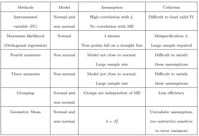
There are a number of commonly used methods to estimate the slope param-eter of the ME model. None of these methods solves the estimation problem in varying situations. A summary of the well known methods is provided in
Table 1.
iii
Table 1: A summary of commonly used methods to handle the ME model problem
Methods Model Assumption Criticism
Instrumental Normal and High correlation withξ. Difficult to fond valid IV
variable (IV) non normal No correlation with ME
Maximum likelihood Normal λknown Misspecificationλ.
(Orthogonal regression) True points fall on a straight line Large sample required
Fourth moments Non normal Model not close to normal. Difficult to satisfy
Large sample size these assumptions
Three moments Non normal Model not close to normal. Difficult to satisfy
Large sample size these assumptions
Grouping Normal and Groups are independent of ME Less efficiency
non normal
Geometric Mean Normal and Unrealistic assumption,
non normal λ=β12 too restrictive sensitive
to error variances
to compare the new estimators and the relevant existing estimators under
different conditions.
One of the most commonly used methods to deal with the ME model is the instrumental variable (IV) method. But it is difficult to find valid IV that is highly correlated to the explanatory but uncorrelated with the error term.
iv
this method is demonstrated both analytically and via numerical as well as
graphical illustrations under certain assumptions.
In Chapter 5, a commonly used method to deal with the normal structural model, namely the orthogonal regression (OR) (which is the same the maxi-mum likelihood solution whenλ= 1) method under the assumption of known
λ is discussed. But the OR method does not work well (inconsistent) if λ is misspecified and/or the sample size is small. We provide an alternative method based on the reflection method (RM) of estimation for
measure-ment error model. The RM uses a new transformed explanatory variable which is derived from the reflection formula. This method is equivalent or asymptotically equivalent to the orthogonal regression method, and nearly
asymptotically unbiased and efficient under the assumption that λ is equal to one and the sample size is large. If λ is misspecified the RM method is better than the OR method under the MAE criterion even if the sample size
is small.
Chapter 6 considers the Wald method (two grouping method) which is still widely used, in spite of increasing criticism on the efficiency of the estimator. To address this problem, we introduce a new grouping method based on
v
the reflection of the explanatory variable. The method recommends different
grouping criteria depending on the value of λ to be one or more/less than one. The RG method significantly increases the efficiency of Wald method, and it is more precise than the other competing methods and works well for
different sample sizes and for different values ofλ. Moreover, the RG method also removes the shortcomings of the maximum likelihood method whenλ is misspecified and sample size is small.
The geometric mean (GM) regression is covered in Chapter 7. The GM
method is widely used in many disciplines including medical, pharmacol-ogy, astrometry, oceanography, and fisheries researches etc. This method is known by many names such as reduced major axis, standardized major
axis, line of organic correlation etc. We introduce a new estimator of the slope parameter when both variables are subject to ME. The weighted ge-ometric mean (WGM) estimator is constructed based on the reflection and
the mathematical relationship between the vertical and orthogonal distances of the observed points and the regression line of the manifest model. The WGM estimator possesses better statistical properties than the geometric
mean estimator, and OLS-bisector estimator. The WGM estimator is stable and work well for different values of λ and for different sample sizes.
es-vi
timators by simulation studies. The computer package Matlab is used for
all computations and preparation of graphs. Based on the asymptotic con-sistency and MAE criteria the proposed reflection estimators perform better than the existing estimators, in some cases, even the standard assumption
on λ and sample size are violated.
Certification of Dissertation
I certify that the ideas, designs and experimental work, results, analyses and
conclusions set out in this dissertation are entirely my own effort, except where otherwise indicated and acknowledged.
I further certify that the work is original and has not been previously
submit-ted for assessment in any other course or institution, except where specifically stated.
Signature of Candidate
Signature of Principal Supervisor
Acknowledgments
My first and foremost thanks to ALLAH for the opportunities that He has given to me throughout my life, especially those that have brought me to the position of finishing this thesis. I would like to express my thankful-ness and gratitude to my principal supervisor Professor Shahjahan Khan for his invaluable assistance, support, patience and guidance during the period of my research, without his knowledge and assistance this study would not have been successful. My special thanks and gratitude go to my associate supervisor Dr Trevor Langlands for his advice, support, constructive feed-back and invaluable assistance. I would like to thank all the staff in the faculty of health, engineering and sciences specially the staff of the school of agricultural, computational and environmental sciences and the library for providing a very good scientific environment for statistical research.
This thesis is dedicated to the souls of my mother and father (may ALLAH bless them with Jannah), that I wish them to be alive to see what I have achieved and to share my happiness for completing this thesis, who always supported, encouraged and directed me for higher education.
Contents
Abstract i
Acknowledgments viii
List of Figures xv
List of Tables xviii
List of Notations xx
Chapter 1 Introduction 1
1.1 Introduction . . . 1
CONTENTS x
1.3 Outline of the Thesis . . . 10
Chapter 2 Historical background of measurement error mod-els 17 2.1 Introduction . . . 17
2.2 Major Axis Regression (Orthogonal) . . . 18
2.3 Deming Regression Technique . . . 20
2.4 Grouping Method . . . 22
2.5 Reduced Major Axis . . . 27
2.6 Moments estimators . . . 30
2.6.1 Estimators based on the first and second moments . . . 30
2.6.2 The method of higher-order moments . . . 38
2.6.3 Estimation with cumulants . . . 46
2.7 Instrumental Variables . . . 50
2.8 Method based on ranks . . . 53
CONTENTS xi
2.10 Structural equation modelling . . . 60
2.11 Other contributions . . . 62
Chapter 3 The reflection approach to measurement error model 64 3.1 Introduction . . . 64
3.2 Methodology . . . 65
3.3 Residuals analysis by reflection technique . . . 66
3.3.1 An alternative proof . . . 70
3.4 Advantages of using reflection . . . 72
3.5 Concluding remarks . . . 88
Chapter 4 Instrumental variable estimator for measurement error model 89 4.1 Introduction . . . 89
4.2 Measurement error models . . . 90
CONTENTS xii
4.3.1 Instrumental variable (IV) estimator . . . 94
4.4 Proposed new IV estimator . . . 96
4.4.1 Geometric Explanation . . . 99
4.5 Some properties and relationships . . . 101
4.6 Illustration . . . 103
4.6.1 Yield of Corn Data . . . 103
4.6.2 Hen Pheasants Data . . . 106
4.7 Concluding Remarks . . . 109
Chapter 5 Reflection method of estimation for measurement error models 111 5.1 Introduction . . . 111
5.2 Orthogonal regression method . . . 114
5.3 Proposed reflection method of estimation . . . 116
5.3.1 Geometric explanation . . . 118
CONTENTS xiii
5.5 Simulation studies . . . 126
5.6 Concluding remarks . . . 131
Chapter 6 Reflection in grouping method estimation 133 6.1 Introduction . . . 133
6.2 Wald’s grouping method . . . 134
6.3 Proposed reflection grouping method . . . 138
6.3.1 Propose modifications to Wald’s method . . . 146
6.3.2 Example . . . 149
6.4 Simulation studies . . . 150
6.4.1 First study: Non-normal distributions of ξ . . . 151
6.4.2 Second study: Normal distributions of ξ . . . 154
6.5 Concluding remarks . . . 158
CONTENTS xiv
7.2 Relationship between the vertical and orthogonal distances . 162
7.2.1 Fitted line case . . . 164
7.2.2 Unfitted line case . . . 166
7.3 Geometric mean estimator . . . 168
7.4 Alternative view on the geometric mean estimator . . . 170
7.5 Proposed estimator . . . 171
7.6 Simulation studies . . . 172
7.7 Concluding remarks . . . 176
Chapter 8 Conclusions 178 8.1 Conclusions and Summary . . . 179
Bibliography 182
List of Figures
3.1 Graph of a reflection point about the OLS regression line of y
onx. . . 71
4.1 Graph representing the sum of squares and products in the
presence of measurement error in the explanatory variable. . . 101
4.2 Graph representing the sum of squares and products when the measurement error in the explanatory variable is ’treated’ by reflection. . . 102
5.1 Graph of the sum of squares and products of the latent and
LIST OF FIGURES xvi
5.2 (a) Graph of the slope estimated and (b) Graph of MAE of
the RM, OR, and OLS estimators ofβ1, when λ= 1 is correct
and small sample sizes 10< n <30. . . 130
5.3 (a) Graph of the slope estimated and (b) Graph of MAE of the RM, OR, and OLS estimators for β1, when λ(= 1.44) is
incorrect and larger sample sizes 10< n <120. . . 131
6.1 Graph of the estimated slope (a) and the mean absolute error (b) for five different estimators whenλ = 1, and β1 = 1. . . 151
6.2 Graph of the estimated slope (a) and the mean absolute error (b) for five different estimators whenλ >1, and β1 = 1. . . 152
6.3 Graph of the estimated slope and the mean absolute error for
five different estimators whenλ <1, and β1 = 1. . . 153
6.4 Graphs of the estimated slope (a) and the mean absolute error (b) for four different estimators RG1, M L, W, and OLS for
case I. . . 155
6.5 Graphs of the estimated slope (a) and the mean absolute error
(b) for four different estimators RG2, M L, W, and OLS for
LIST OF FIGURES xvii
6.6 Graphs of the estimated slope and the mean absolute error for
four different estimators RG3, M L, W, and OLS for case III. 157
7.1 Graph of two orthogonal distances (AB=Od, andAD =Ox) between the observed point and the fitted and unfitted lines. . 163
7.2 Graph of three estimators of the slope, and the mean absolute error when β0 = 20, β1 = 0.55 and 0.08≤λ≤100. . . 173
7.3 Graph of three estimators of the slope, and the mean absolute
error when β0 = 27, β1 =−0.75 and 0.08≤λ≤100. . . . 174
List of Tables
1 A summary of commonly used methods to handle the ME
model problem . . . iii
4.1 Fitted regression models for the corn yield data . . . 104
4.2 Fitted regression models for the Hen peasants data . . . 107
5.1 The simulated mean of five different estimators and the MAE
when β1 = 1, β0 = 0, n = 100. . . 128
5.2 The simulated mean of five different estimators with the MAE when β1 = 2, β0 = 0, n = 100. . . 128
6.1 Estimated β1 and β0 for different estimators when both
LIST OF TABLES xix
7.1 Simulated mean values of the estimated slope and the mean
List of Notations
ξj Unobserved explanatory variable (latent variable).
ηj Unobserved response variable (latent variable).
xj Observed explanatory variable (manifest variable).
yj Observed response variable (manifest variable).
x∗j Reflection of the observed explanatory variable.
y∗j Reflection of the observed response variable (manifest variable). δj Measurement error in the explanatory variable.
ϵj Measurement error in the response variable.
ej Equation error in the true model.
vj Equation error in the Measurement Error model.
ψ Reflection angle about the unfitted regression line (by manifest variables).