Volume 2, No. 5, Sept-Oct 2011
International Journal of Advanced Research in Computer Science
CASE STUDT AND REPORT
Available Online at www.ijarcs.info
Two-Phase Great Deluge Algorithm for Course Timetabling Problem
Allen Rangia Mushi
Department of Mathematics University of Dar es salaam Dar es salaam, Tanzania [email protected]
Abstract: Academic course timetabling involve assigning resources such as lecturers, rooms and courses to a fixed time period, normally a week, while satisfying a number of problem-specific constraints. This study describes a Great Deluge Algorithm in two phases that creates timetables by heuristically minimizing penalties over infeasibilities. The algorithm is developed with special focus on the University of Dar-as-salaam and compares the results with a previous work on Tabu Search, and a manually generated solution. We conclude that Great Deluge gives a much more stable solution because it produces good solutions with less number of parameters for tuning compared to Tabu Search.
Keywords: Course Timetabling, Great Deluge, Tabu Search
I. INTRODUCTION
There are many types of timetabling problems ranging from high schools, to universities and industries. Most of these problems are NP-Hard [1] which makes it difficult to obtain timetables that meet all user needs. Schaef [2] and Burke et al [3] gives a survey of automated timetabling where they summarize types of problems and varying efforts in automating solutions. University timetables are basically of two types; courses and examinations. These two are significantly different and requires different algorithms for their solutions. In this study we investigate course timetabling which essentially is the problem of finding an assignment of courses, rooms, students and lecturers to a fixed time period, normally a five-day week, while satisfying a known number of constraints. These constraints are divided into hard and soft, where hard constraints must be satisfied, while soft constraints are to be satisfied as much as possible. One interesting feature of University Timetabling is that, the properties vary from one university to another. Although similar features can be generalized, the solution for one university may not necessarily work in another. In this paper, course timetabling at the University of Dar es salaam (UDSM) is used as a case study.
Since this problem is NP-Hard, most of the research work concentrates on heuristic approaches. Genetic algorithms have been reported by many authors including Burke et al [3],[4], Colorni et al [5], Rossi and Paechter [6], Jain A., Jain S, Chande P [7] and Hiroaki, Uochi, Takahashi, Miyahara [8]. Simulated Annealing has been applied with variations depending on the specific features of the problem such as ElMohamed and Fox, [9] and Kostuch P [10]. Tabu Search is also found in the literature including White and Xie [11]. Ant colony algorithm is an attempt to mimic the behavior of ants when searching for the shortest path to a food source and going back to their original stations by laying substances called pheromones. A few attempts have been made on Ant Colony algorithms, including the work by Rossi and Paechter [6]. However, most of these heuristic algorithms require a huge discipline and experimentation in the selection of parameters which are often very specific to a problem. Furthermore, these parameter values have great influence in the performance of the algorithm. Slight change in
parameters might lead to a significantly large change in the solution values. Mushi A [12] presents a Tabu Search approach to the UDSM course timetabling and concludes that careful selection of parameters is important for success of the algorithm. Such a conclusion is common to many popular heuristic techniques including Simulated Annealing and Genetic Algorithms. This prompted researchers to think of heuristic algorithms which are less dependent on parameters and therefore more stable. Great Deluge algorithm is in this category and was proposed by Dueck [13]. Other such algorithmic techniques in this category include Late Acceptance [14] and its variants such as Average Late Acceptance [15] and Adapted randomized Late Acceptance [16]. An exploration of the Great Deluge algorithm for possible use in course timetabling was firstly presented by Burke et al [17]. However, their algorithm was specifically designed for a set of timetable rules designed for International Timetabling competition, which are not standard to all timetabling applications. A variant of the algorithm which uses an non-linear decay rate is proposed by Landa-Silva and Orbit [18][19] and applied to a set of problems designed for a timetabling competition. Due to its robustness, Great Deluge has been combined with other techniques and applied to various timetabling problems with good success [20]. In this work we are interested in the Basic Great Deluge algorithm which is implemented in two phases for exploration of UDSM problem instances.
In the next section, we introduce the actual course timetabling problem at UDSM, followed by a discussion on the Great Deluge algorithm. Then we present the specific implementation details, followed by summary of results and conclusion.
II. PROBLEMDEFINITION
laboratories, 650 lecturers, and 10,000 students to be scheduled on a five days week. Each day is made up of 13 one-hour time slots starting from 7.00 a.m. to 8 p.m. giving a total of 65 timeslots for the whole timetable period. No consideration is given to the lunch breaks except on Fridays which are minimally used to allow for Muslim prayers.
The current practice is to use commercial software which provides a set of tools that the timetable officer can use to simplify the process. The timetable is essentially created manually, using a set of tools that can help to detect collisions and suggest suitable slots. This is a long process and a semester timetable takes an average of three weeks to prepare given that all necessary data have been entered into the system.
The main challenge is to automate the timetabling process and come up with a quick and optimized timetable. Due to unforeseen problems such as untimely data, it is not possible to ignore the manual process all together; the output of the automated system will however provide a highly advanced solution which can easily be modified by the manual systems afterwards. Major challenges include the annual increase of number of students, and high freedom of course choice among students. The problem is also compounded by an increasing number of faculty-wide and university-wide courses which requires large rooms and special timeslots.
The following terminologies are used in this paper; a) Course – A set of subject content to be taught to a
particular group of students.
b) Event – An assignment of lecturer, room and a course to a one hour time interval. A course can have several events according to the number of hours set in the curriculum.
c) Lecture – A set of events of the same course, which are required to be scheduled together in the same room and the same time. A lecture can have one or more events. d) Block – A lecture with more than one consecutive
events.
A. Hard constraints:
a. No student can attend more than one lecture at a time b. No lecturer can teach more than one lecture at a time c. No room can occupy more than one lecture at a time d. No room can be assigned a lecture with more students
than its capacity
e. Some courses are scheduled in blocks of more than one hour, these restrictions must be respected.
B. Soft constraints:
a. As much as possible, minimize the use of early morning (7.00 a.m.) lunch hours (13-14) and late evening hours (18-20).
b. Specifically minimize the use of Friday 13-14 hour and 18-20 hour slots to allow for Muslim prayers and Adventists Seventh day respectively.
c. Minimize continuous lectures/blocks of the same course in a day. It is preferred to spread them over the week as much as possible.
d. Minimize the use of rooms with no standby generators in the evening. This is to minimize the loss of lecture hours due to power cuts which are common in the area. e. Satisfy as much as possible the special preferences by
lecturers, students and University administration.
III. SOLUTIONAPPROACH
A. Great Deluge Algorithm:
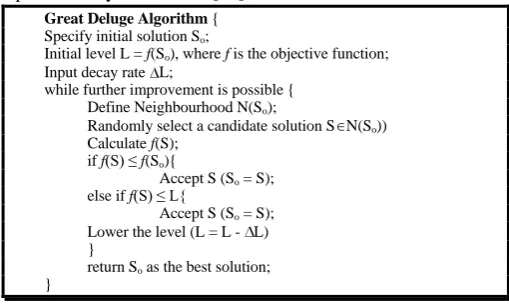
The original idea is based on a maximization problem, where one is trying to search for solution on a space. The process then involves moving around randomly on the space, but there is a “water level” below which the solution cannot be searched. If this level is given by L, then a solution S is accepted at any point only if S > L. As time goes on, L rises slowly and finally the solution is forced up to the peak and stops. The algorithm can easily be mapped to a minimization problem. Petrovic and Burke [21] have shown how this algorithm can be mapped into timetabling problems with a minimization objective function. Generally, the algorithm can be outlined by the following pseudo-code (Figure 1), as presented by Burke et al [17];
Great Deluge Algorithm { Specify initial solution So;
Initial level L = f(So), where f is the objective function; Input decay rate L;
while further improvement is possible { Define Neighbourhood N(So);
Randomly select a candidate solution S N(So)) Calculate f(S);
if f(S) ≤ f(So){
Accept S (So = S); else if f(S) ≤ L{
Accept S (So = S); Lower the level (L = L - L) }
[image:2.595.308.563.237.389.2]return So as the best solution; }
Figure 1: Great Deluge Algorithm
Great Deluge algorithm always accept better solution than current, but can accept worse solutions if the evaluation function value is less than or equal to the level L. The decay rate is the only input parameter required and it determines the
speed of level reduction. In a time-predefined
implementation, one can decide beforehand the number of iterations needed for convergence and calculate the value of decay rate. If we define Lo to be the initial level value, and
) (Sf
f to be the final expected objective value, then L can
be calculated as follows;
iter f
N S f L
L 0 ( ), where Niter is the desired number of
iterations. The initial level is normally assigned the value of initial cost, but the final value can only be proposed depending on the type of objective function. As it will be seen in the next section, our objective function is structured in such a way that the best possible value is zero. Thus the
value of L is simply calculated by
iter
N L
L 0 and Niter
becomes the new input parameter. Thus, the algorithm only requires one input value i.e. the estimated number of iterations, Niter.
B. Adapting Great Deluge to UDSM Course Timetabling:
a) Data Representation :
i. Solution: Given a total of n events, a timetable solution
is represented as integer-valued matrix
S
n 3such thatS
sei is a solution for event e and attribute i, where
e event to allocated Room 2 e event to allocated Timeslot 1 e event with associated Course 0 i
ii. Courses: Represented by a matrix Cm3 such that
C
cij stands for course i with attribute j, where
size imum block units course size course j max 3 2 1
Each course has been designed with a fixed number of units which determines the number of hours to be delivered per week for that course. Each unit stands for one lecture hour per week, so that a 2 units course requires 2 lecture hours per week. Some courses have restrictions on the number of consecutive hours (block) per each delivery. Maximum block size helps to determine the number of blocks required for a course. For instance, a 3 unit course with a maximum block of 2 hours will need one block of 2-hours and an extra one hour event.
iii.Rooms: Represented by an array R such that
r
iR
is the capacity of room i.iv. Collision matrix: Note that, two courses i and j clashes if they have at least one student or lecturer in common. Thus, given a set of m courses, we define a conflict matrix
M
m m such thatOtherwise j i mij 0 course with clashes course if 1
Checking for a possible student/lecturer clashes between courses i and j simply involves finding the value of
M
m
ij .v. Objective function:
Given a solution s, and a set of k constraints; k
i i if s s f Minimize 1 ) ( ) ( ,
Each function
f
i represents one of the constraints andeach i is the weight given to the constraint depending on its importance. The cost function includes both hard and soft constraints, but higher penalties are assigned to hard constraints to discourage them from being selected.
b) Constraints :
Full description of the formulation of each constraint is found in Mushi A [12]. It only suffices here to give a summary of the formulations for the sake of continuity.
Recall from the definitions of data structures above;
0
e
s
= course associated with event e1
e
s
= timeslot allocated to event e2
e
s
= room allocated to event e And let E = set of all timetable events, Then the constraints are;i. No student or lecturer can have two lectures at the same time.
Minimize 1f1(s), where
j i S S E j i ij j i M s f 1 1 ) , (
1( ) , which is
the total number of collisions associated with the current solution. A feasible solution must havef1(s) 0.
ii. Only one event can be assigned to a room at a time.
Given
Otherwise
0 if
1 i2 j2
ij
s s
a , minimize 2f2(s) , where
j i s s E j i ij j i a s f 1 1 ) , (
2( ) which is the total number of room
clashes in the current solution. Again a feasible solution must havef2(s) 0.
iii. Room capacities must be respected. Given i se0, and
2
e
s
r , and
Otherwise r Cap i Cap if bir 0 ) ( ) ( 1
, where
) (j
Cap Capacity of object j, minimize 3f3(s), where
e ir E ir b s f ) , (
3( ) , i.e. the total number of room size
violations in the current solution. Obviously, f3(s) 0 is a necessary condition for feasibility.
iv. Maximize the distance between two events or block of events of the same course.
Minimize 4f4(s),
where j i s s E j
i i j si sj s f 0 0 ) , ( 2 1 1 4 ) ( 1 )
( . The best possible
value for f4(s) is 0.
v. Minimize the use of special times.
Let H = set of all special timeslots and
minimize; 5f5(s), where
H e
e s s
f5( ) 1. This is the sum of
all timeslots for courses which have been assigned to the less desired times. The best possible value of f5(s) is 0 i.e. the case where no course violates the special times.
vi. Minimize the use of rooms with no standby generators in the evenings.
Given G = set of all rooms fitted with standby generators and V = set of all evening (18-19) timeslots of the week, and
define
Otherwise G s V se e e 0 if
1 1 2
, then minimize 6f6(s),
where;
e e s
f6( ) . This calculates the total number of
events which have violated the standby generator constraint in the current solution. When all courses satisfy this constraint,
f
6(
s
)
must have a value of 0.Consequently, the best value of the overall objective
function is obtained when ( ) ( ) 0.
1
k
i i if s s
f
c) Generating Initial timetable :
algorithm simply involves assigning each event to the earliest possible feasible timeslot and earliest feasible room. To help reduce the risk of developing an infeasible solution, both courses and rooms are sorted in descending order of their sizes. Note that a timetable is feasible if satisfies all hard constraints.
d) Neighbourhood and Move types :
The performance of any local search strategy requires a good decision on the choice of neighborhood. Our neighborhood is defined by the type of moves that we have implemented. There are two types of attributes that we can vary in order to get a different solution i.e. timeslots and rooms. Assuming fixed rooms from the initial solution, we can move timeslots. On the other hand, we can fix timeslots and change rooms. This prompted us to consider a two phase process, where phase I considers fixed rooms and perform timeslot changes, and Phase II fixes timeslots and vary rooms in search of a better solution. Basically, room move is useful only when phase I did not bring a feasible solution, as this may be caused by infeasible room allocations. However, our selection of moves for phase II affects both timeslots and rooms, which increases the chance of finding a feasible and better solution. The two types of moves are as defined below;
i. Timeslot move:
This affects only the timeslots as follows;
a. Select a random event e in the set of all possible events
b. Select randomly a new timeslot t in the set of all possible timeslots.
c. Assign the new timeslot t to the event at position e. If e is a member of a block of events, assign t to all timeslots of the block.
Such a move is identical to several moves described in literature [22][23]. The size of the neighborhood associated with this kind of move is |N(s)| = |e| (|t|-1), where |e| = total number of events, and |t| = total number of timeslots.
ii. Event swap move:
a. Swap of two events from different courses as follows; b. Select randomly two event e1, e2 in the set of all possible
events of different courses
c. Find whether it is possible to swap; it is possible to swap events only if they have the same block size.
d. If possible to swap, then swap course numbers of the two event blocks otherwise select another set of events and repeat 1 until swap is successful.
The size of the neighborhood associated with this kind of move is |N(s)| = |e| (|e|-1). As pointed earlier, this type of move affects both timeslots and rooms since a course is associated with both a timeslot and room number.
e) Stopping criteria:
Apart from the pre-defined number of iterations from the calculations of the decay value L, it has been found that there is a possibility of further improvement even after level has dropped to zero. We have therefore added condition which considers the number of consecutive iterations without a change in solution value. The algorithm stops after running 1000 iterations without solution change.
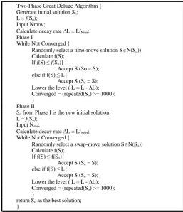
The two-phase algorithm is therefore as presented in Figure 2;
Two-Phase Great Deluge Algorithm { Generate initial solution So; L = f(So);
Input Nmov;
Calculate decay rate L = L/Niter; Phase I
While Not Converged {
Randomly select a time-move solution S N(So)) Calculate f(S);
If f(S) ≤ f(So){
Accept S (So = S); else if f(S) ≤ L{
Accept S (So = S); Lower the level ( L = L - L); Converged = (repeated(So) >= 1000); }
Phase II
So from Phase I is the new initial solution; L = f(So);
Input Niter;
Calculate decay rate L = L/Niter; While Not Converged {
Randomly select a swap-move solution S N(So)) Calculate f(S);
If f(S) ≤ f(So){
Accept S (So = S); else if f(S) ≤ L{
Accept S (So = S); Lower the level ( L = L - L); Converged = (repeated(So) >= 1000); }
[image:4.595.307.565.54.353.2]return So as the best solution; }
Figure 2: Two-phase Great Deluge Algorithm
The decay rates in the two phases are different, depending on the performance of phase I; basically it is expected to have fewer moves in the second phase, since phase I will considerably reduce the search space. This modification has the implication of increasing the number of parameters to two, i.e. Niter values for phase I and II.
However, the total number of parameters is still low compared to other heuristics such as Tabu Search or Simulated Annealing.
IV. COMPUTATIONALRESULTS
[image:4.595.338.545.578.646.2]The algorithm was tested on a course timetabling problem previously solved by manual methods. The code is written in C++ and test run on a 2.9 GHz Pentium processor. Table 1 shows data for the specific problem used in the test runs;
Table 1: Data for the tested problem at UDSM
Data Value
Students 8161
Lecturers 607
Rooms 106
Courses 729
Total events 1570
Total timeslots 65
Table 2: Weights used in the objective function
Weight Value Description
1 - 3 100 Hard constraints
4 10 Distance between events
5 4 Friday Muslim prayers
4 Seventh day Adventists
2 Lunch times
1 Morning and evening times
6 3 Standby generators
The author is the coordinator of timetable at UDSM and therefore these weights were assigned according experience on the importance given to various factors at UDSM. The same problem and weights were used in the Tabu Search case [12]. As in Tabu Search case, time move performed much better than event swap. Table 3 shows the performance of the algorithm for the time moves tested and compared to Tabu Search. The rows of the table show the kind of constraints solved and their performance in the final solution. Both values are the average of performances for different randomly generated values using different seeds in the random number generator.
Table 3: Performance of the Algorithm
Initial cost C0: 2894.72 Great Deluge Tabu Search
Event swap Time move
Phase I cost 141.36 1.74
Final Cost 1.98
Student/Lecturer Collisions 0 0
Room clashes 0 0
Room size 0 0
Event Distance 1.98 1.74
Special time penalties 0 0
Standby generators 0 0
Time (Seconds) 7,826.73 4,684.91
% Improvement 99% 99%
The best solution was found after 7,826.73 seconds which is about 2 hours and 17 minutes; that is a tolerable range in timetabling applications. The final solution is significantly close to the one obtained by Tabu Search. The Great Deluge solution however, is much more stable. The improvement achieved in Phase II is very significant showing the usefulness of the two-phase approach.
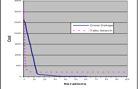
Figure 3 shows the performance improvement by iterations and compare with previous results for Tabu Search. Although Tabu Search finally converges to a lower solution value (Table 3), the graph shows that Great Deluge can provide a better solution in the higher levels. Most of the time is spent on the lower levels of iterations with minimal improvement. Thus the values of Niter can be adjusted to stop
the algorithm within a tolerable range as needed by the timetable officer without great loss in the quality of solution.
0 500 1000 1500 2000 2500 3000 3500
1 11 21 31 41 51 61 71 81 91 101
Ite r ations
Co
st
Great D eluge T abu Search
Figure 3: Performance improvement by iterations
[image:5.595.34.279.303.426.2]A comparison with a manually generated solution is provided in Table 4. It provides a summary of the performances in terms of constraint violations. It is worth noting that both cases were feasible by satisfying all hard constraints. However, the course-event gaps and special time penalties could not work very well in the manual system which involves mostly trial and error method.
Table 4: Manual vs Automatic Performances
Constraints Violations in Manual
Violations in automatic
Student/Lecturer Collision 0 0
Room clashes 0 0
Room size violations 0 0
Course event gaps 253.75 1.98
Special time penalties 659 0
Standby generators 0 0
Total violation cost 912.75 1.98
% Improvement from Co 71% 99%
V. CONCLUSIONANDFURTHERRESEARCH DIRECTIONS
We have successfully demonstrated that, Great Deluge can give a robust solution without significant loss in the quality of solution. Generally, the automatic solution generation strategies perform better than purely manual solution. Although human intervention may still be necessary in the final automatic solution generated, the algorithm it still provides a significant improvement in the final overall solution.
Timetabling research area is widely explored but still leaves a load of research opportunities since the problems are always specific to particular institutions. Furthermore, most of these problems involve a huge list of soft constraints which may not be possible to implement all at a time. New constraints may arise from time to time and provide new challenges to researchers especially in academic institutions which are always trying to improve their programmes and administrative structures. In developing countries, the problem is compounded further by scarcity of resources which desperately need optimization so as to provide the much needed education to as many students as possible. An exploration of general features within developing countries and thereby coming up with a general template which can be customized to fit different institutions in the form of a decision support system could be very useful in improving education systems. Many algorithms have been tested recently but only on a few case studies; further testing of these algorithms in new problems especially in developing countries could be interesting and worth investing.
VI. REFERENCES
[1] Cooper T., Kingston J. “The Complexity of Timetable Construction Problems”, 1996, Springer Lecture Notes in Computer Science 1153, pages 283-295
[2] Schaef A, “A Survey of Automated Timetabling”, CWI Report CS-R9567, 1995, Netherlands
[image:5.595.39.280.612.764.2][4] Burke E., Elliman D., Weare R.: “A Hybrid Genetic Algorithm for Highly Constrained Timetabling Problems”, In Morgan Kaufmann (Ed): Proceedings of the sixth International Conference of Genetic Algorithms, Pittsburgh USA, 15-19th July 1995, pp. 605-610.
[5] Colorni A., Dorigo M., Maniezzo V.: “Genetic Algorithms and Highly Constrained Problems: The Timetable case”, Proceedings of the First International Conference on Parallel Problem Solving from Nature, Dortmund, Germany, 1991, Lecture Notes in Computer Science 496, Springer-Verlag, pp. 55-59.
[6] Rossi-Doria O., Paechter B.: “An Hyper heuristic approach to course timetabling problem using an evolutionary algorithm”, The 1st Multi-disciplinary International Conference on Scheduling: Theory and Applications (MISTA 2003), August 2003.
[7] Jain A., Jain S., Chande P., “Forumlation of Genetic Algorithm to Generate Good Quality Course Timetbale”, International Journal of Innovation, Management and Technology, Vol. 1, No. 3, pp. 248-251, 2010.
[8] Hiroaki U., Uochi D., Takahashi K., Miyahara T.: “Comparisons of Genetic Algorithms for Timetabling Problems”, Systems and Computers in Japan, 2004, Vol. 35, No. 7.
[9] ElMohamed M., Fox G., “A Comparison of Annealing Techniques for Academic Course Scheduling”, Practice and Theory of Automated Timetabling II, 1998, Selected Papers from the 2nd International Conference, PATAT'97, Edmund Burke and Mike Carter (Eds.), Lecture Notes in Computer Science, Springer
[10]Kostuch P.: “The University Course Timetabling Problem with a 3-phase approach”, Proceedings of the 5th International Conference on the Practice and Theory of Automated Timetabling, Pittsburgh, USA, 2004.
[11]White G., B. Xie, :”Examination Timetabling and Tabu Search with longer term memory”. In E. Burke and W. Erben, (Eds.), 2001, The Practice and Theory of Automated Timetabling III, Lecture Notes in Computer Science 2079, pp. 85-103, Springer-Verlag.
[12]Mushi A. R.: “Tabu Search Heuristic for University Course Timetabling Problem”, African Journal of Science and Technology, Science and Engineering Series, 2006, Vol. 7, No. 1, pp. 34-40.
[13]Dueck G.: “New Optimization Heuristics: The Great-Deluge Algorithm and the Record-to-record Travel”, Journal of Computational Physics, 1993, Vol. 104, pp. 86-92.
[14]Burek E., Bykov Y., “A Late Acceptance Strategy in Hill-Climbing for Exam Timetabling Problems”. In Proceedings of PATAT’08, Proceedings of the 7th
International Conference on the Practice and Theory of Automated Timetabling, Universit de Montral, Montreal Canada, 2008.
[15]Abuhamdah A., Ayob M., “Average Late Acceptance Randmosized Descent Algorithm for Solving Course Timetabling Problems”, Proceedings of the 4th
International Symposium on Information Technology, Selangor, Malaysia, IEEE, 2(15-17), pp. 748753, 2010.
[16]Abuhamdah A., Ayob M., “Adaptive Randomized Descent Algorithm for Solving Course Timetabling Problesm”, International Journal of the Physical Sciences, Vol. 5(16), pp. 2516-2522, 2010.
[17]Burke E., Bykov, Y., Newall J., Petrovic S.: “A Time-Predefined Approach to Course Timetabling”, Yugostlav Journal of Operational Research (YUDOR), Vol 13 No. 2., pp. 139-151, 2003.
[18]Land-Silva D., Orbit J., ”Great Deluge with Non-Linear Decay Rate for Solving Course Timetabling Problems”. In Proceedings of the 2008 IEEE Conference on Intelligent Systems (IS 2008), pp. 8.11 – 8.18, IEEE Press, Los Alamitos.
[19]Orbit J., Landa-Silva D, “Computational Study of Non-Linear Great Deluge for University Course Timetabling”. In V. Sguev (Ed): Intelligent Systems: From Theory to Practice, SCI 299, pp. 309-328, Springer-Verlag, 2010.
[20]Nabeel R., “Hybrid Genetic Algorithms with Great Deluge for Course Timetabling”, IJCNS International Journal of Computer Science and Network Security, Vol. 10, No. 4, pp. 283-288, 2010
[21]Petrovic S., Burke E.: “University Timetabling”, In Leung J. (Ed): Handbook of Scheduling Algorithms, Models and Performance Analysis, 2004, Chapter 45, CRC Press. [22]Reeves C.: “Landscapes. Operators and Heuristics Search”,
Annals of Operations Research, 1999, Vol. 86, pp. 473-490. [23]Thomspon J., Dowsland K.: “Variants of Simulated