1
School of Business, James Cook University 2
School for Environmental Research, Charles Darwin University
Socio-Economic Activity and Water
Use in Australia’s Tropical Rivers:
A Case Study in the Mitchell and
Daly River Catchments
Prepared by Natalie Stoeckl1, Michelle Esparon1, Owen Stanley2, Marina Farr1, Aurélie Delisle1 and
Zulgerel Altai1
Disclaimer
TRaCK has published the information contained in this publication to assist public knowledge and discussion and to help improve the sustainable management of Australia’s tropical rivers and coasts. Where technical information has been prepared by or contributed by authors external to TRaCK, readers should contact the author(s), and conduct their own enquiries, before making use of that information. No person should act on the contents of this publication whether as to matters of fact or opinion or other content, without first obtaining specific independent professional advice which confirms the information contained within this publication.
While all reasonable efforts have been made to ensure that the information in this publication is correct, matters covered by the publication are subject to change. Charles Darwin University does not assume and hereby disclaims any express or implied liability whatsoever to any party for any loss or damage caused by errors or omissions, whether these errors or omissions result from negligence, accident or any other cause.
Copyright
This publication is copyright. Apart from any fair dealing for the purpose of private study, research, criticism or review as permitted under the Copyright Act, no part may be reproduced, by any process, without written permission from the publisher, Enquiries should be made to the publisher, Charles Darwin University, c/- TRaCK, Casuarina Campus, Building Red 1 Level 3, Darwin NT 0909.
TRaCK brings together leading tropical river researchers and managers from Charles Darwin University, Griffith University, the University of Western Australia, CSIRO, James Cook University, the Australian National University, Geoscience Australia, the Environmental Research Institute of the Supervising Scientist, the Australian Institute of Marine Science, the North Australia Indigenous Land and Sea Management Alliance, and the Governments of Queensland, the Northern Territory and Western Australia.
TRaCK receives major funding for its research through the Australian Government's Commonwealth Environment Research Facilities initiative; the Australian Government's Raising National Water Standards Program; Land and Water Australia; the Fisheries Research and Development Corporation and the Queensland Government's Smart State Innovation Fund.
Stoeckl, N., Esparon, M., Stanley, O., Farr, M., Delisle, A., and Altai, Z. (2011). Socio-Economic Activity and Water Use in Australia’s Tropical Rivers: A case Study in the Mitchell and Daly River Catchments. Charles Darwin University, Darwin.
For further information about this publication: Natalie Stoeckl, James Cook University
Or to find out more about TRaCK
Visit: ISBN: 978-1-921576-37-9
Socio-Economic Activity and Water
Use in Australia’s Tropical Rivers:
A Case Study in the Mitchell and
Daly River Catchments
Final Report for
The Tropical Rivers and Coastal Knowledge Research
Consortium
March 2011
Data caution
Every effort has been made to collect regionally relevant data from robust samples of people and industries in the Daly River and Mitchell River catchments.
Some of the data used in the models were collected by members of the research team. As is almost always the case when conducting surveys, one cannot be 100 per cent sure that the sample data are truly representative of the underlying population, and this document discusses some of the data collection problems encountered during this project.
Much of the data used in the models is secondary, having been collected by the Australian Bureau of Statistics (ABS) during the 2006 Census, and by the ABS for their water accounts. Two problems are particularly pertinent to this report:
1) One of the most significant problems associated with ABS Census data on Indigenous persons is that of ‘undercount’1, and our models use ABS data on employment and incomes of Indigenous and Non-Indigenous people, by sector, in each catchment. As such, it is important to acknowledge that the absolute numbers reported in this document would be different if more accurate employment data were used. The most likely scenario, is that our models overstate the extent of Indigenous disadvantage. But it is extremely unlikely that ‘more accurate’ data would alter any of the main ‘punch-lines’ findings of our research (namely that: there is a significant, and asymmetric divide between Indigenous and Non-Indigenous economic systems; that different industries generate quite different income, employment and water-use outcomes; and that Agriculture, and perhaps also mining are key sectors to monitor if concerned with consumptive water use in these regions - see comments in point 2, below).
2) Estimates of water use by industry/sector were obtained from the ABS Water accounts. However, as noted by the Northern Australia Land and Water (NALW) taskforce (2009, p 23) “mining and resource projects are generally excluded from water resource accounting, exact water use estimates for this industry are not readily available”. We thus encourage users to treat our estimates with caution unless, and until, the water use estimates associated with the mining sector can be verified. Those caveats aside, it is important to note that alternative sources of data, suitable for analysis in these types of models, at this scale, in these regions, do not exist. So whilst it must be openly acknowledged that the data used in this research are imperfect, they are, arguably, better than the alternative (nothing). Moreover, as detailed in relevant sections of this report, there is at least some accord/consistency between the employment and water use data collected in our household survey and that collected by the ABS. This gives some credence to the numbers. As such, this project represents a step forward. But it is a very modest step. There is considerable room for improvement: until that occurs, results must be taken as indicative only, and not interpreted as precise estimates.
1
There are significant problems with the quality of data relating to Indigenous people (Australian Human Rights Commission,
Acknowledgements
We gratefully acknowledge and appreciate the contribution to this research made by Mitchell River Catchment Traditional Owners (The Olgol, the Yir Yoront, The Western Gugu Yalanji; The Mulliridgee; The Barbarum, The Kuku Djunkan and Gugu Mini, and by the Daly River Catchment Traditional Owners living in Kybrook Farm and Pine Creek and Nauiyu Nambiyu (Daly River).
A special thank you is also due to
The community of Kowanyama, particularly:
• Viv Sinnamon - Kowanyama Aboriginal Land and Natural Resource Management Office • Michael Yam-Shire - Councillor, Former chair of Mitchell River Watershed Management
Group, Member Mitchell River Traditional Custodians Advisory Group and Olgol TO • Anzac Frank - Kowanyama Aboriginal Ranger and Yir Yoront TO
• Ravin Greenwool - Kowanyama Aboriginal Ranger: Cultural Heritage and Kin Kopol / Yir Yoront TO
• Phillip Mango and Stanley Budby - Kowanyama Aboriginal Rangers
The Mitchell River Traditional Custodian Advisory Group, particularly • Ruth Link - Chair and Western Gugu Yalanji TO
• Gerry Turpin - Treasurer and Mbabaram TO
• The people of Western Gugu Yalanji, Kuku Juungan, Mbabaram and Wokomin.
The Daly River Aboriginal Reference Group (ARG), particularly: • Mona Liddy
• Valemina White
The TO’s who worked with us so diligently when collecting data:
• Darren Birchley - Kowanyama Aboriginal Ranger and Kokoberra TO • Sharon Brady - Western Gugu Yalanji TO
• John Grainer - Kuku Djungan TO • Eddie Turpin – Mbabaram TO • Eddie Thomas – Wokomin TO • Agnes Page
• Kathleen Perry • Bridget Kikitin; and • Lizzie Sullivan
The Tropical Savannas CRC – for their in-kind data contribution.
Pippa Featherston, Emma Woodward and Sue Jackson for their invaluable, and timely help, conducting interviews in the Daly River Catchment.
Executive Summary
Tropical Rivers and Coastal Knowledge (TRaCK) is a research hub that was established in 2007 under the Commonwealth Environment Research Facilities Program. Its aim is to provide the science and other knowledge that governments, communities and industries need for the sustainable use and management of Australia’s tropical rivers and estuaries. Section 1, Project overview:
One of the research activities undertaken by TRaCK is the description and analysis of the ways in which the components of the socio-economic system interact with each other, and with the environment in the tropical rivers (TR) region. The report presents the results of that research. While some of the research was concerned with the TR region overall, more intensive analysis was conducted for the two focal catchments of the Daly River (NT) and the Mitchell River (Qld).
The TR region is approximately 15 per cent of Australia’s mainland but it is home to fewer than 2 per cent of all Australians. Most of the TR region is sparsely populated, with two-thirds of the population living in urban centres and larger localities, of which Darwin is the largest. The population composition is unusual, by comparison with the rest of Australia: with a higher than average Australian male/female ratio, and a younger average age. Almost one-third of the usual residents in the TR region are Indigenous, compared with just two per cent nationally. In terms of the catchment under study, 28 per cent of the Daly River population is Indigenous while 23 per cent of the Mitchell River catchment population is Indigenous.
Section 2, Background to the Tropical Rivers Region and to the two focal catchments:
While the average population turnover rate between 2001 and 2006 is about the same as that for Australia overall, it was very high for Darwin and the Southern Gulf parts of Queensland and lower along the east coast of the Northern Territory and between the Embley and Coleman River catchments in Queensland. Generally, Non-Indigenous people are much more mobile than rural Indigenous people.
Overall land use in the TR region is dominated by conservation and natural environments. In the Daly catchment, for instance, grazing makes up 54 per cent of land use and 39 per cent of the land remains under what is formally classified as being in “natural condition”: of which 27 per cent is specifically designated as traditional Indigenous use and 5 per cent is set aside for conservation. The remaining land uses are divided among dryland agriculture (5 per cent), intensive uses such as urban, mining or industrial (1 per cent) and irrigated land (1 per cent). In the Mitchell catchment, 95 per cent of land use is directed towards production from unchanged land (i.e. grazing); 3 per cent of the land is in natural condition and almost exclusively under conservation, and land under intensive use (including urban, mining, industrial) is minimal at 0.03 per cent. Interestingly, there is no natural land solely reserved for Indigenous use in the Mitchell as opposed to the Daly.
After extensive consultation with stakeholders and other researchers, and a thorough examination of existing models that could be used or adapted, it was decided to build an Input-Output (IO) model for each catchment that would differ from the usual IO model in two ways. Firstly, the household sector in each model was divided into Indigenous and Non-Indigenous households. The Non-Indigenous/Non-Non-Indigenous split allows the impacts of change to be measured for those two groups separately. Secondly, the IO models involved the modeling of water use for individual industries and households.
Sections 3 and 4 – Identifying an appropriate modeling technique, and refining the methodological approach:
Data for Non-Indigenous households were obtained from a mail-out survey in the two focal catchments, while most of the data for the Indigenous households were obtained from during face-to-face interviews. Other data required for this modeling were obtained from the ABS and from an earlier, associated, survey of businesses in Northern Australia. Much of the data had to be ‘transformed’ prior to use, and where ever possible, data were compared with other related data sources (e.g. the ABS’s household expenditure survey) to test plausibility prior to inclusion in the model.
Section 5 – Operationalising the models and populating them with data:
The models were used to estimate Type I and Type II income multipliers (defined in section 4), and also employment and water multipliers. In addition to considering aggregate impacts, the analysis looked at the distributional impacts of change, providing the following insights:
Section 6.1 – using the models to estimate income, employment and water multipliers:
• A one-dollar increase in final demand in almost any business sector generates a net increase in regional income of between $1.60 and $2.40, depending upon the sector. Most of that money (i.e. at least $1.00) stays within the sector that is initially stimulated, but there are flow-on effects to other sectors.
• In most cases, it is the Finance sector (which, in this model, includes property and business services), the Retail sector (including both retail and wholesale trade) and Non-Indigenous households which benefit most from ‘flow-on’ effects. In most cases, these sectors receive approximately $0.20 each. In stark contrast, Indigenous Households generally receive just a few cents in flow-on effects; approximately one-half of one per cent of the total regional stimulus, and just one per cent of the total flow-on effects.
• The largest flow-on increase in Indigenous incomes occurs if one stimulates the Government sector, but even there, the flow-on effect is just $0.05 following a $1.00 initial increase.
• When Indigenous incomes are increased exogenously (which could occur, for example, via an increase in royalty payments or an increase in Centrelink payments), Non-Indigenous people capture more of the flow-on effects than do Indigenous people. A $1 exogenous increase in Indigenous incomes results in Indigenous people gaining a flow-on benefit of just $0.01 - $0.03, whereas Non-Indigenous people gain a flow-on increase of $0.18 - $0.26.
• Stimuli affect the labour market in a similar manner: economic growth always creates significantly more jobs for Non-Indigenous householders than Indigenous householders. These differences are not entirely attributable to differences in population.
• There are also significant differences in water multipliers across different industries. Water multipliers in the Agricultural sector are orders of magnitude larger than those in other sectors, although care must be taken when interpreting data relating to the Mining and Manufacturing sector: as noted by the NALW taskforce (2009, p 23) “mining and resource projects are generally excluded from water resource accounting, exact water use estimates for this industry are not readily available”. Consequently, the estimates presented here may understate – perhaps grossly – actual figures for the mining sector.
• There is a marked difference between the water-use multipliers that have been estimated using upper and lower-bound water use coefficients. To the extent that water is at least partially substitutable with other resources (e.g. it is possible to reduce water use and still grow certain types of plants by, for example, mulching, or applying water at critical phases of a plant’s growth cycle), these results clearly illustrate the importance of water-saving technologies and research, particularly in the agricultural sector.
The models were also used to examine the possible impact of different types of economic growth in the catchments. The models were used to calculate results for one year, and then extrapolated for the next 20 years. The results were as follows:
Section 6.2 – using the models to explore various growth scenarios:
1. The ‘balanced’ growth scenario (of 1.5 per cent per annum across all industries) significantly out-performed all other scenarios for employment and income in the Daly. It was one of the top two generators of income and employment in the Mitchell (alongside the 5 per cent growth in Agriculture scenario). Within 20 years, this scenario increased Industry Income and Non-Indigenous Employment to levels that were close to 1.6 times greater than in 2006. Indigenous employment outcomes were more modest – rising to between 1.4 and 1.5 times the 2006 levels. This balanced growth scenario was also associated with moderate increases in consumptive water demand – rising to between 1.2 and 1.7 times 2006 levels depending upon whether one used lower or upper bound estimates.
2. In the Mitchell River, growth in the Agricultural sector generated substantial increases in business/industry incomes and in Non-Indigenous employment. Outcomes for Indigenous people were much more modest. If growth in Agriculture is achieved using water-efficient techniques (‘mimicked’ here, with the lower-bound water use coefficients), then in 2026, our models predict that consumptive water demand would be just 1.6 times greater than 2006 levels; but consumptive water demand could be more than double 2006 levels in less than a decade if higher water-use coefficients prevail.
3. Income and employment outcomes associated with the Agricultural scenario were more modest in the Daly than in the Mitchell, but pressures on consumptive water demand were similar in both catchments. Outcomes for Indigenous people (incomes and employment) were also very modest in both regions – rising by less than 10 per cent, in total, over a 20 year period.
5. The mining scenario delivered marginally better household income and employment outcomes to both Indigenous and Non-Indigenous households than did the tourism scenario, but the returns were still quite small. In contrast, the associated increase in industry output/incomes were relatively good and even out-performed those of the agricultural scenario in the Daly River. The predicted increases in consumptive water demand were similar for the mining and tourism scenarios. However, as noted earlier, these simulations may under-estimate (perhaps substantially) the amount of consumptive water demand associated with the mining sector.
These results are important to anyone involved in, or interested in, northern economic development. They provide an indication of the downstream benefits from the stimulation of any industry, though not, of course the costs of such stimulation. Whilst the results of our analysis are only directly associated with two focal catchments, many other catchments in the region are socioeconomically ‘similar’. As such, the key messages (if not precise estimates) may be relevant across many northern regions. These key messages are:
Section 7 – Discussion and concluding comments:
1) There is an asymmetric divide between Indigenous and Non-Indigenous economic systems in Northern Australia. Given the lack of employment and business opportunities, workplace skills, and the other infrastructure prerequisites for development, local Indigenous people are very unlikely to benefit from the stimulus of any of the north’s existing industries. This situation is likely to persist unless, or until, there is structural change.
2) Some industries may be able to generate significant business income and/or incomes for some householders, but will not necessarily deliver significant localised benefit in terms of, for example, employment (be it Indigenous or otherwise). Development strategists may thus need to explicitly acknowledge these tradeoffs and make conscious decisions about what it is they wish to ‘develop’ (e.g. Regional income or regional employment? Regional income or Australian income?). Moreover, strategists may need to think about innovative methods of redressing some of the potential problems arising from such tradeoffs, ensuring that the methods allow for the structural idiosyncrasies of these small northern economies (i.e. the asymmetric divide noted above).
3) Water multipliers differ by orders of magnitude depending upon assumptions made about the numbers of litres of water consumed per dollar output particularly in the Agricultural sector. This clearly highlights the fact that water-saving technologies are vitally important.
4) Both Agriculture and mining are capable of generating significant income flows. But, unlike growth in the government, health or educational sectors, growth in the agricultural sector2
.
is associated with significant growth in consumptive water demand. Development strategists may thus also need to explicitly acknowledge some of the non-monetary impacts of different development options (not all of which will be negative), seeking to identify ways in which to exploit synergies, redress tradeoffs, and thus capitalise on opportunities that do not place un-due strain upon the region’s natural resources (water being but one of many important examples).
2
TABLE OF CONTENTS
EXECUTIVE SUMMARY ... 6
1 PROJECT OVERVIEW ... 14
2 SOCIO-ECONOMIC BACKGROUND ... 17
2.1 THE TR REGION ... 17
2.2 THE CASE STUDY CATCHMENTS ... 20
2.2.1 General description ... 20
2.2.2 Land Use ... 22
2.2.3 Employment ... 23
2.2.4 Similarities and Differences between these, and other catchments ... 23
3 IDENTIFICATION OF AN APPROPRIATE MODELING APPROACH ... 24
3.1 STAKEHOLDER CONSULTATIONS ... 24
3.2 OVERVIEW OF MACROECONOMIC MODELS ... 25
3.3 SELECTION OF MODELING APPROACH ... 27
4 METHODOLOGICAL DETAILS ... 30
4.1 CONCEPTUALIZING THE MODEL... 30
4.1.1 The basic IO model ... 30
4.1.2 Differentiating between Indigenous and Non-Indigenous Households ... 31
4.1.3 Incorporating Water Use ... 34
4.1.4 Allowing for employment ... 34
4.2 A CAUTION ABOUT THE INTERPRETATION OF RESULTS ... 35
5 OPERATIONALIZING THE MODEL ... 36
5.1 DEFINING SECTORS ... 36
5.2 POPULATING THE MODEL WITH DATA ... 37
5.2.1 The (Leontief) matrix B: Business and organizational expenditure ... 37
5.2.2 The matrix C: Household expenditure ... 39
5.2.3 The matrix V: Value added ratios ... 53
5.2.4 The vector w: Direct water use ... 55
5.2.5 The matrix E: Direct use of Indigenous and Non-Indigenous employees ... 62
6 RESULTS... 65
6.1 ESTIMATING MULTIPLIERS ... 65
6.1.1 Type I and Type II income multipliers ... 65
6.1.2 Indigenous and Non-Indigenous Employment multipliers ... 69
6.1.3 Water multipliers ... 71
6.2 SIMULATING THE EFFECTS OF DIFFERENT TYPES OF GROWTH ... 73
6.2.1 Establishing a baseline ... 73
6.2.2 Specifying the growth scenarios ... 76
6.2.3 Simulation outputs ... 80
7 DISCUSSION ... 85
8 CONCLUDING COMMENTS ... 88
APPENDIX 1 – HOUSEHOLD EXPENDITURE AND WATER USE SURVEY ... 89
APPENDIX 2 – INDIGENOUS HOUSEHOLDS’ INTERVIEW ... 95
APPENDIX 3 – INTRODUCTORY LETTER SENT TO HOUSEHOLDS ... 102
APPENDIX 4 – REMINDER LETTER ... 104
APPENDIX 5 – FACTSHEET ... 105
TABLE OF FIGURES
Figure 1 - The tropical rivers region of Australia ... 14
Figure 2 – Conceptual model underpinning the investigations of Project 3-1 ... 15
Figure 3 - Populations of urban centers and larger localities in the TR region ... 17
Figure 4 - Population mobility, 2001-2006 ... 18
Figure 5 - Projected age-specific contribution to growth for the TR region, 2006 to 2026 (%) ... 19
Figure 6 - The two focal catchments of the modeling activity ... 20
Figure 7 - Age-sex pyramid in the Daly and Mitchell River catchments by Indigenous status, 2006. ... 21
Figure 8 - Changes in age cohorts in the Daly and Mitchell River catchments from 1996 to 2006 (%) ... 22
Figure 9 - Land use in the TR region, primary level of ALUM classification ... 22
Figure 10 – Similarities and differences between the focal catchments and other catchments in the TR region. . 23
Figure 11 - Conceptualization of the circular flow of income – importing stock from outside ... 25
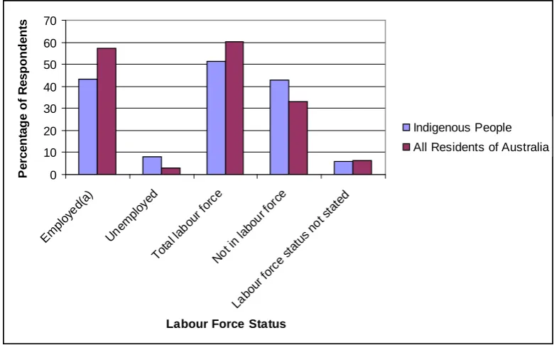
Figure 12 - Indigenous versus Non-Indigenous labour force status ... 32
Figure 13 - IO, Demand, Supply and Price ... 35
Figure 14– Average household size – by catchment and Indigenous status ... 42
Figure 15 – Age composition of household – by catchment and Indigenous status ... 42
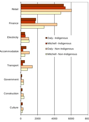
Figure 16 – Mitchell River Employment by sector and Indigenous status – ABS and Household Survey data compared ... 43
Figure 17 – Daly River Employment by sector and Indigenous Status – ABS and Household Survey data compared ... 44
Figure 18 – Weekly Household expenditure on different goods and services – by Catchment and Indigenous Status ... 45
Figure 19 – Household Expenditure patterns in the Daly and Mitchell catchments compared with national data . 47 Figure 20 – Per person expenditure patterns in the Daly and Mitchell catchments compared with national data . 48 Figure 21 - Annual expenditure per person - by ANZSIC sector and catchment ... 49
Figure 22 – ‘Local’ expenditure per person per annum ... 51
Figure 23 – Estimated aggregate income received from different business sectors by Indigenous Status – Mitchell River ... 55
Figure 24 – Estimated aggregate income received from different business sectors by Indigenous Status – Daly River ... 55
Figure 25 – Mitchell River and Daly River Multipliers Compared ... 65
Figure 26 – Indigenous and Non-Indigenous employment ‘multipliers’ by sector – Daly River ... 70
Figure 27 – Indigenous and Non-Indigenous employment ‘multipliers’ by sector – Mitchell River ... 71
Figure 28 – Water ‘multipliers’ by sector – Daly River ... 72
Figure 29 – Water ‘multipliers’ by sector – Mitchell River ... 72
Figure 30 - Mining/Exploration Sites in the TR region ... 79
Figure 31 – Demographic Scenario – Mitchell River ... 81
Figure 32 – Demographic Scenario – Daly River ... 81
Figure 33 – Growth scenarios in the Mitchell River ... 83
Figure 34 – Growth scenarios in the Daly River ... 84
Figure 35 – The great asymmetric divide ... 86
TABLE OF TABLES
Table 1 – The focal catchments’ profile ... 21
Table 2 - Overview of Applied Australian Models (non-exhaustive list) ... 27
Table 3 - Number of ‘observations’ on business expenditure per sector in the Mitchell, Daly and TR regions ... 38
Table 4 – Number of householders covered in survey compared to estimated population – by Indigenous status and catchment ... 41
Table 5 – Highest level of education completed by any member of the household – per centage of households by Indigenous status and catchment ... 43
Table 6 – Mean Household Income and Mean Income per person – by Indigenous status and catchment (A$ per annum) ... 51
Table 7 – Per cent of total income spent with LOCAL industries – by Indigenous status and catchment (%) ... 52
Table 8 – 2006 Persons Employed – by ANZIC sector, catchment and Indigenous Status ... 53
Table 9 – 2006 Median weekly Income – by ANZIC sector, catchment and Indigenous Status ... 54
Table 10 – 2000-01 Water consumption (ML, 2000-01) – by sector and state ... 57
Table 11 – Gross Value Added ($M, 2000-01) – by sector and state... 57
Table 12 – Litres of water consumed per $GVA – by sector and state ... 58
Table 13 – Land use in the Northern Territory ... 58
Table 14 –Industry water Use Coefficients for WIO models ... 59
Table 15- Calculation of average water use consumption per household ... 60
Table 16 - Average litres of water used per person per day – by catchment and Indigenous status ... 62
Table 17 – Household water Use Coefficients for WIO models ... 62
Table 18 – 2006-07 GVA, Employment and Employment per $M GVA for QLD ... 63
Table 19 – 2006-07 GVA, Employment and Employment per $M GVA for NT ... 63
Table 20 – 2006-07 Persons Employed per $M GVA – by sector, catchment and Indigenous Status ... 63
Table 21 - MITCHELL RIVER - Total change in output/incomes following a one-unit change in final demand within a single sector ... 67
Table 22 - DALY RIVER - Total change in output/incomes following a one-unit change in final demand within a single sector ... 68
Table 23 – Estimated Household Income by catchment and Indigenous status (A$ per annum) ... 74
Table 24 – Estimating industry GVA for the Mitchell River ... 74
Table 25 – Estimating industry GVA for the Daly River ... 75
Table 26 – Estimated total water consumption by sector and by catchment (ML, 2006)... 76
Table 27 – Estimating the change in household expenditure that is likely to occur in conjunction with changes in population – by catchment... 77
ABBREVIATIONS AND ACRONYMS ABS ANZSIC CDEP CGE CPI CRC CSIRO DRMAC EIO EPA GRP GVA HES IO JCU LWA MRTCAG NALW NGO NT NWI OGS QLD SAM TO TR TRACK WIO US
Australian Bureau of Statistics
Australian and New Zealand Standard Industrial Classification Community Development Employment Project
Computable General Equilibrium model Consumer Price Index
Cooperative Research Centre
Commonwealth Scientific and Industrial Research Organisation Daly River Management Advisory Group
Environmental Input-Output Environmental Protection Agency Gross Regional Product
Gross Value Added
Household Expenditure Survey Input-Output
James Cook University Land and Water Australia
Mitchell River Traditional Custodial Advisory Group Northern Australian Land and Water
Non Government Organisation Northern Territory
National Water Initiative
Office of the Government Statistician Queensland
Social Accounting Matrix Traditional Owners Tropical Rivers
Tropical Rivers and Coastal Knowledge Water-use Input-Output model
United States Accommodation Agriculture Communications Construction Culture Education Electricity Finance Government Health Manufacturing Mining Personal Property Retail Sewerage Transport Wholesale
Accommodation, Cafes, Restaurant Agriculture, Forestry and Fishing Communications Services Construction and Trade Services Cultural and Recreational Services Educational Services
Electricity, Gas and Water Supply Finance and Insurance
Government Administration and Defense Health and Community Services Manufacturing
Mining, Quarries and Related Services Personal and Other Services
Property and Business Services Retail Trade
1 Project overview
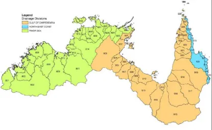
[image:14.595.90.506.174.429.2]The tropical rivers (TR) region comprises 55 river basins in two major drainage divisions (see Figure 1). Covering an area of more than 1.3 million km2, it extends across all catchments from the east side of Cape York to the Kimberley, through Queensland, the Northern Territory and Western Australia. It includes some of Australia’s largest river systems which are – by area size – the Flinders, Roper, Victoria and Fitzroy Rivers and – by volume – the Nicholson and Mitchell Rivers (NGIS Australia, 2004).
Figure 1 - The tropical rivers region of Australia
In 2004 the Board of Land and Water Australia (LWA) identified Australia’s TR region as a priority area for major investment over the subsequent five years. Later that year a process of dialogue, consultation, and negotiation with Indigenous communities, stakeholders, governments and researchers commenced to develop a shared vision for a “Tropical Rivers Program”.
The aim was:
“To undertake research and knowledge exchange to support the sustainable use, protection and management of Australia’s tropical rivers”3
(Land and Water Australia, 2008) Subsequently, the Tropical Rivers and Coastal Knowledge (TRaCK) research hub was established in 2007 under the Commonwealth Environment Research Facilities Program. Its aim was to provide the science and knowledge that governments, communities and industries need for the sustainable use and management of Australia’s tropical rivers and estuaries (TRaCK, 2008).
The TRaCK research program has seven main themes exploring the environmental, social, cultural and economic consequences for rivers, coasts and communities of potential developments and climate change. (See the TRaCK website for a detailed description of the themes)
3
• Theme 1: Scenario evaluation • Theme 2: Assets and values
• Theme 3: River and coastal settings • Theme 4: Material budgets
• Theme 5: Foodwebs and biodiversity • Theme 6: Sustainable enterprises • Theme 7: Knowledge and adoption
The research about which this report is written was undertaken by those involved in TRaCK Project 3.1, “Socio-economic activity and water use in the TR region”. The project is a component of Theme 3, the overarching objectives of which are to:
i. develop a physical template based on hydrological regime and geomorphology to characterise, classify and understand the formation of riverscapes and estuaries; ii. understand the demographic and social character of human populations within
catchments and the relationship with the physical template; and
iii. relate the potential of biophysical character to attract and sustain different development pressures.
Project 3.1 focuses primarily on objective (ii) and seeks to improve our understanding of the demographic and socio-economic character of the human populations within catchments and their relationship with the physical template. It also contributes to objective (iii) in that it explores the potential consequences (on incomes, employment and consumptive water demand) of a variety of different development ‘options’.
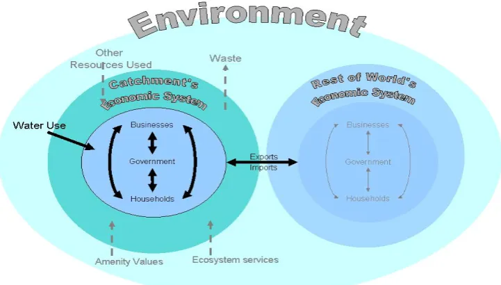
[image:15.595.118.479.452.657.2]The conceptual model underlying this project (adapted from Common and Stagl (2005), p 87) is shown in Figure 2 below. It hypothesises that there are multiple economic systems which are embedded within social systems which are, themselves, embedded within the broader environment (i.e. within an ecological system) and that there are multiple ways in which the systems interact.
Figure 2 – Conceptual model underpinning the investigations of Project 3-1
The research work related to Project 3.1 was divided into three ‘activities’, with each investigating a different aspect of that conceptual model.
developed tourism and population profiles and projections for the entire TR region, and for each individual catchment within the TR region. It also identified key issues affecting population (resident and tourism) growth for the period of 2006 to 2015. Section 2.1 of this reports presents a few key highlights from that investigation, but readers are encouraged to peruse the full set of results in Carson et al. (2009).
The second activity set out to describe the ‘contents’ of the region’s socio-economic systems. It compiled data on key socio-economic characteristics of the region as a whole, and developed profiles of individual TR catchments (based on their socio-economic characteristics). Individual catchment-level profiles were compared and contrasted to identify socio-economically ‘similar’ and ‘dissimilar’ catchments. Section 2.2 presents a few key highlights from that investigation, and interested readers are encouraged to see the full results in Larson and Alexandridis (2009).
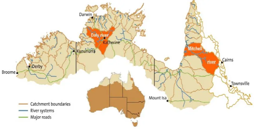
The final activity (and the one on which this report focuses) set out to describe the way in which different components of the socio-economic systems interact with each other, and with the environment. Focusing on just two catchments within the TR region, researchers working on this part of the project developed a Water-Use Input-Output (WIO) model for the Daly River Catchment in the Northern Territory, and the Mitchell River Catchment in Queensland (Figure 6). They used the models to make predictions about the likely changes to Indigenous and Non-Indigenous incomes, employment and to water demand that could occur in response to different types of economic growth (e.g. an increase in mining, agriculture and/or tourism). This activity thus focused primarily on the economic interactions between households and businesses, and on one type of economic/environmental interaction, namely: the amount of water ‘used’ (or, more precisely, ‘demanded’)4.
This report describes the research undertaken to develop those WIO models, and presents some results from a small number of ‘simulations’ derived from them. It is structured as follows.
Section two provides a brief overview of some of the key socio-economic characteristics of the TR region and the two focal catchments, drawing mainly, although not exclusively, upon material published in the final reports of the other two activities that were undertaken as part of project 3.1. Section three briefly describes the investigations undertaken when seeking to identify a modeling approach capable of meeting the project’s objectives, while section four provides some methodological details of the selected modeling approach. Section five carefully describes the way in which the models were populated with data. It presents secondary data, describes the household survey that was undertaken to collect primary data and explains the way in which data (primary and secondary) were converted for use within the models. Section six presents results from the modeling exercises undertaken in this project, while section seven offers some concluding remarks.
4
2 Socio-economic Background
2.1 The TR region
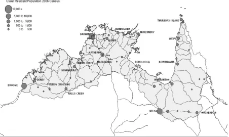
[image:17.595.74.527.206.477.2]Despite the fact that the TR region covers approximately 15 per cent of Australia’s mainland, it is home to fewer than 2 per cent of all Australians. Indeed just 310,000 people, (approximately) had their usual residence in the TR region at the time of the Australian Bureau of Statistics (ABS) 2006 census (Carson et al., 2009). Two-thirds of these people live in urban centres and larger localities (Figure 3).
Figure 3 - Populations of urban centers and larger localities in the TR region
Source: Carson et al., (2009) based on ABS 2006 Census
Most of the TR region is therefore sparsely populated, with all but four basins having less than 1 person per km2. By far, the largest population centre in the region is Darwin. Greater Darwin5 recorded a population of over 100,000, or one-third of the total TR usual resident population at the census (Carson et al., 2009), and in 2006 there were only three communities (Darwin, Mount Isa and Broome) with a population of more than 10,000 and almost half of the TR basins (i.e. 24 basins) had fewer than 500 people.
Carson et al., (2009) noted that the population mix in the region is unusual in comparison with the rest of Australia. The median age for the total region was 33 years, compared with a median age for Australia of 37 years. There were 107 males recorded in the TR region for every 100 females, compared to the national sex ratio of 97. One quarter of the usual residents in the TR region were Indigenous (16 per cent of Australia’s Indigenous population), compared with just two per cent nationally.
With regard to the rates of population turnover experienced in the TR region, it was found to be consistent with those reported across Australia as a whole. There were nearly 2000 more people who moved out of the region between 2001 and 2006 than who moved in to the
5
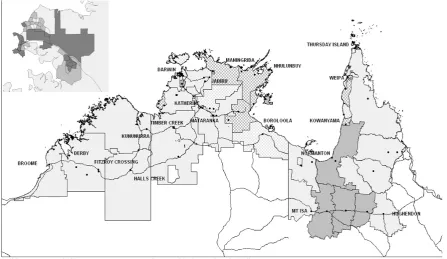
region. However, population turnover rates were not consistent across the region. Carson et al., (2009) identified pockets of very high population turnover in Darwin and the Southern Gulf parts of Queensland (between the Flinders and Mitchell River catchments), and low levels of population turnover along the east coast of the Northern Territory and between the Embley and Coleman River catchments in Queensland (Figure 4).
Solid grey = population turnover rates consistent with the national median, Solid dark grey = high population turnover rates,
[image:18.595.72.520.138.397.2]Hatched grey = low population turnover rates, Inset in the figure = Greater Darwin area.
Figure 4 - Population mobility, 2001-2006
Source: Carson et al., (2009) based on ABS 2006 Census
growth rates (2.13 per annum) are projected for the Non-Indigenous population of the Western Australian regions.
Figure 5 - Projected age-specific contribution to growth for the TR region, 2006 to 2026 (%)
Source: Carson et al., (2009).
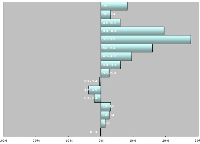
Almost all of the expected future growth (in absolute terms) is likely to be contributed by those aged 40 years and above, particularly by those aged 50 to 64 years (Figure 5). Negative growth in the working age cohorts of 20 to 34 years is expected with only minor growth in the infant cohort (birth to four years). These cohorts are projected to increase their share of the population significantly as the 40 years plus population grows from 38 per cent to 56 per cent.
2.2 The case study catchments
2.2.1
General description
[image:20.595.87.495.125.332.2]The two catchments selected for analysis in this project were the Daly and the Mitchell; depicted in Figure 6.
Figure 6 - The two focal catchments of the modeling activity
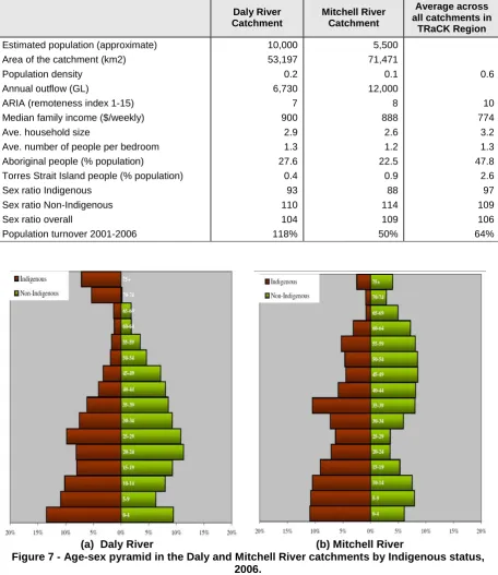
Both the Daly and the Mitchell River catchments cover vast areas, both being larger than the ‘average’ catchment in the TR region. Both catchments are well provisioned in water (in terms of annual outflows which are, on average, greater than the ‘average’ river in the TR region). There is, however, considerable seasonal variation in water flows, and – like most of Northern Australia – both are sparsely populated (see Table 1). The catchments resemble the average TRaCK region in terms of average number of people per bedroom and overall sex ratio: in all cases, there are more males than females. In comparison to an average family in the TRaCK region, families in the Daly and Mitchell enjoy a higher weekly median income. There is however a significant difference in population turnover – from 2001 to 2006, population turnover in the Daly almost doubled that of the average population turnover in the TRaCK region, but the same was not observed in the Mitchell.
Table 1 – The focal catchments’ profile
Daly River Catchment
Mitchell River Catchment
Average across all catchments in
TRaCK Region
Estimated population (approximate) 10,000 5,500 Area of the catchment (km2) 53,197 71,471
Population density 0.2 0.1 0.6
Annual outflow (GL) 6,730 12,000
ARIA (remoteness index 1-15) 7 8 10
Median family income ($/weekly) 900 888 774
Ave. household size 2.9 2.6 3.2
Ave. number of people per bedroom 1.3 1.2 1.3
Aboriginal people (% population) 27.6 22.5 47.8
Torres Strait Island people (% population) 0.4 0.9 2.6
Sex ratio Indigenous 93 88 97
Sex ratio Non-Indigenous 110 114 109
Sex ratio overall 104 109 106
Population turnover 2001-2006 118% 50% 64%
[image:21.595.70.527.63.591.2]
(a) Daly River (b) Mitchell River
Figure 7 - Age-sex pyramid in the Daly and Mitchell River catchments by Indigenous status, 2006.
Source: Carson et al., 2009
(a) Daly River (b) Mitchell River
Figure 8 - Changes in age cohorts in the Daly and Mitchell River catchments from 1996 to 2006 (%)
Source: Carson et al., 2009
2.2.2
Land Use
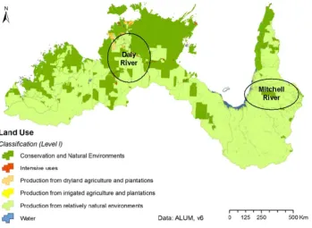
As depicted in Figure 9, overall land use in the TR region is dominated by conservation and natural environments. In the Daly catchment, grazing makes up 54 per cent of land use and 39 per cent of the land remains under natural condition: of which 27 per cent is specifically designated as traditional Indigenous use and 5 per cent is set aside for conservation (Larson and Alexandridis, 2009). The remaining land uses are divided among dryland agriculture (5 per cent), intensive uses such as urban, mining or industrial (1 per cent) and irrigated land (1 per cent).
Figure 9 - Land use in the TR region, primary level of ALUM classification
Source: Larson and Alexandridis, 2009
exclusively under conservation, and land under intensive use (including urban, mining, industrial) is minimal at 0.03 per cent. Interestingly, there is no natural land solely reserved for Indigenous use in the Mitchell as opposed to the Daly.
2.2.3
Employment
Across the entire TRaCK region, the Government Services sector accounts for 25 per cent of employment; the next most significant sector of employment is Agriculture, Forestry and Fishing (11.5 per cent), while Mining, Retail and Construction each comprise around 4 per cent of the labour force (Larson and Alexandridis, 2009). The same general pattern of employment is observed in both the Daly and Mitchell catchments (Larson and Alexandridis, 2009; see also Table 8). However, in the Daly catchment, the importance of the Government Services sector is much more notable. In comparison to the Mitchell catchment, fewer people are employed in the Agriculture, Forestry and Fishing sector (4 per cent as opposed to 15 per cent).
2.2.4
Similarities and Differences between these, and other catchments
Using 5 different data sets, and three different statistical methods, Larson and Alexandridis (2009) clustered catchments across northern Australia, based on their socio-demographic and economic characteristics. Figure 10 provides a pictorial summary of key results from the clustering exercise that used a full set of data. It shows catchments which were identified as being socio-economically ‘similar’ in ‘similar’ shades/colours, and catchments which were identified as being socio-economically ‘dissimilar’ in contrasting shades/colours. Full details of their analysis are contained within their report – suffice to say here, some catchments which are 1000’s of kilometers distant have more in common with each other, than with their ‘next door neighbours’.As regards the Mitchell River – its socio-economic characteristics are similar to those of the Flinders; the Daly River is most similar to the Fitzroy and the Ord. It is, therefore, possible, that the models described in this report could provide information relevant to a larger group of catchments (and people) than just those in the Daly and the Mitchell.
Figure 10 – Similarities and differences between the focal catchments and other catchments in the TR region.
3 Identification of an appropriate modeling approach
As noted in the introduction, researchers involved in this part of the project were tasked with the job of developing a model that could be used to describe the way in which different components of the socio-economic system interact with each other, and with the environment. It was also deemed desirable to develop a model that could be used to ‘simulate’ the outcomes of different types of development (e.g. more Agriculture, more Mining).
In the first instance, this required researchers to identify the most appropriate type of economic model(s) to use. Specifically, they needed to:
(a) identify the types of socio-economic variables that stakeholders would like to have information about when considering the ‘impacts’ of different types of development; and the ‘changes’ (to variables) that stakeholders would like to model the impact of;and (b) determine which economic model(s) could best meet those needs.
There was an initial literature search that identified generic modeling options. This was followed by discussions with other TRaCK researchers and TRaCK’s Knowledge and Adoption team which helped determine which ‘generic’ modeling option seemed most promising. Finally, there was a more detailed search of the literature and available data – the primary aim of which was to determine how best to build the desired model (given the many available approaches, and the time-frames involved in the project). Further details are given below.
3.1 Stakeholder consultations
In April 2008, Prof Stephen Garnett and Neil Collier, met with the Daly River Management Advisory Committee (DRMAC), and sent other researchers a summary of key issues discussed during that workshop. The summary identified general development scenarios that were of interest to DRMAC. Furthermore, researchers involved in Project 3.1 consulted with several TRaCK researchers – gaining particularly valuable insights with respect to key issues confronting those living in both the Daly and the Mitchell River catchments. Researchers involved in Project 3.1 had also been involved in a previous study – funded by the Tropical Savannas Cooperative Research Centre (CRC) which canvassed the views of 148 different individuals associated with a broad range of stakeholder groups (local, state and federal government departments; non-government organizations (NGO’s), Indigenous associations, etc) across Australia’s North with respect to their socio-economic modeling needs (Stoeckl and Stanley, 2005). This background information thus allowed for the following observations:
a) There was clear interest in information about incomes and jobs. Most interest seemed to be at a fairly broad sector/industry level (e.g. Mining, Tourism) but there was an indication that stakeholders would like more detailed information in some sectors, particularly for Agriculture and for the household sector (specifically looking for Indigenous / Non-Indigenous split).
b) Additionally, there was clear interest in economy/environment interactions – e.g. in water consumption, water pollution, cultural and recreational water use, aquifer use, etc.
(sectoral) models selected for development must also be able to deal with economy/environment interactions.
3.2 Overview of macroeconomic models
The economy-wide impact of a change (say ‘growth’ or extra expenditure) in a particular sector is often greater than the initial amount of ‘growth’ or expenditure. The process by which this happens can best be explained by use of an example. Let us suppose that a visitor to a regional town spends some money that had been earned outside the region at a local grocery store. As such, the owner of the store sees their business ‘grow’ by $100. He/she may put aside some money for savings/profit (say $10) and for taxation (say $20). He/she may also spend money importing stock from outside the region, e.g. Cairns (say $30), and may spend the rest on wages or on fresh produce from the local gardener (say $40).
Figure 11 depicts the process diagrammatically – clearly showing that the total regional stimulus of the $100 of tourist expenditure is greater than $100: it is equal to the $100 earned by the grocer, plus the $40 earned by the gardener. Indeed the final regional stimulus may even be higher than $140, depending upon how much money the gardener spends within the local economy.
Figure 11 - Conceptualization of the circular flow of income – importing stock from outside
The advantage of looking at the process conceptually is that it is easy to see that the size of the final economic stimulus generated by the ($100) ‘growth’ of the tourism sector depends, at least in part, on the spending pattern of those within the region of enquiry. The larger the proportion of any ‘extra’ income re-spent within the local region, the greater the overall regional benefits of that initial tourist expenditure (or, in economic terminology, the greater the regional multiplier). Consequently, those wishing to explore the macro-economic consequences of different types of development (e.g. growth in tourism, mining, agriculture or some other sector) need information about the financial links and expenditure patterns of local firms and households.
The ‘theoretically preferred’ way to explore development options is to build a Computable General Equilibrium (CGE) model – although many researchers use Input-Output (IO)
A tourist spends $100 at the local store
The store owner earns and extra $100
The store owner saves some of that money - $10
The store owner has to give some of that money to the government in
taxes - $20
The store owner spends $30 importing stock from Cairns The store owner spends
$40 on locally grown vegetables
models. Further details concerning IO models are provided in section 4, but suffice to say here, IO models are basically simplified CGE’s. They use historical data about the way in which different types of businesses (or sectors) have previously spent money to make predictions about what might happen across an entire region if there were an increase or decrease in economic activity. An IO model that contained data like that in Figure 11, would, for example, predict that an increase of $100 in tourist expenditure would generate an increase in regional incomes of at least $140 (more, if the local gardener spends some of his/her money locally).
‘Standard’ IO models (and some of the simple CGE’s) require researchers to accept many questionable assumptions, but there are more sophisticated models and techniques available. For example, IO analysis has been adapted to allow for dynamic relationships (Leontief and Duchin, 1986; Nabors, Backus, and Amlin, 2002; Robinson and Duffy-Deno, 1996). The models can also be extended to consider distributional impacts – using what is termed a Social Accounting Matrix (SAM) – see Berck and Hoffman, (2002), and they are also able to allow for multiple regions – e.g. the Core-Periphery models of Hughes and Holland (1994). Furthermore, models can allow for non-linear relationships between inputs and outputs (Liew, 2000; Wang, 2001).
Most pertinent to this project, is the fact that IO models (and, CGE’s) can also be extended to include economy-environment interactions (Eder and Narodoslawsky, 1999; Gustavson, Lonergan, and Ruitenbeek, 1999; Hawden and Pearson, 1995; Huang, Anderson, and Baetz, 1994; Lenzen and Foran, 2001; O’Doherty and Tol, 2007). These ‘interactions’ are important because – as noted in the introduction – economic systems are essentially sub-systems of socio-economic sub-systems which are sub-sub-systems of the broader natural environment, and there are many ways in which the economic system affects, and is affected by, the broader environment. Figure 2 (presented in the introduction) provides examples of different types of economic/ environment interactions, including situations where the economic system:
(a) uses the environment as a ‘dump’ (e.g. emitting pollution); (b) extracts resources from the environment (e.g. water);
(c) benefits from the environment’s ecosystem services (e.g. recreation); and (d) benefits from the (non-consumptive) use of the environment’s amenities (e.g.
beauty).
The first attempt to incorporate economic/environment interactions into an IO model occurred in the late 1960s, when the ‘standard’ IO model was extended to allow for the environment by simply adding a row that measured pollution emissions per sector. Although criticized in some quarters, this “simple method of adding a set of row vectors in the Input-Output table has been widely adopted for investigating the environmental emissions or resource consumption triggered by economic development” (Guan and Hubacek, 2008, p 1301).
Since the 1960s there have been several attempts to develop IO models that could account for a wide variety of economic/environment interactions – like those associated with (a) – (d) above. However, most have been severely hampered by lack of data, particularly when dealing with ecosystem services and/or amenity values. Indeed it seems that the successful investigations have, by and large, restricted themselves to accounts of (a) resource flows from the environment to the economy, and/or (b) the flow of wastes from the economy to the environment (Victor, 1972; Jin et al., 20036
6
Cited in Guan and Hubacek, 2008.
resources extracted from the environment and the environmental damage caused by the economy (Common and Stagl, 2005, p104)7
3.3 Selection of modeling approach
.
Table 2 provides an indicative list of a range of different applied macro-economic models currently in use in Australia. Although this country is host to many world-class models, none provide information at a fine geographic scale in the North. There is only one model that explicitly accounts for consumptive water use – but it is highly aggregated (looking at all of Australia). Even the most regionally detailed model (TERM) only provides data for statistical divisions. These are geographically large in Northern Australia; encompassing, for example, almost all of Northern Territory (except the area in and around Darwin).
Table 2 - Overview of Applied Australian Models (non-exhaustive list)
MODEL NAME REGION TYPE OF MODEL GENERAL DESCRIPTION
GRIMP8
(Grit Impact Program)
Australia Input-Output An Input-Output model using cross sectional data by industrial sector. Can simulate impact on output (or employment or energy etc) of a change in final demand. Lenzen and Foran
(2001)
Australia Input-Output with Water Use
An Input-Output model that explicitly accounts for the consumptive water use of each sector.
ORANI9 Australia Comparative static single region CGE
An applied general equilibrium model first developed in the 1970’s. It has largely been superseded by the MONASH suite of CGE models.
ORANI-NT Australia and the NT
Comparative static multi-region CGE
A comparative static multi-region model based on ORANI. QGEM10 (Queensland General Equilibrium Model) Australia and Queensland
Comparative static multi-region CGE
A CGE model developed by Queensland Treasury to assess the impacts of policy changes and shocks. The QGEM-T model variation specifically looks at the tourism sector.
MMR11 (Murphy Model Regional)
Australia Comparative static multi-region CGE
MMR is a CGE model of the Australian economy used for regional policy analysis. It can be used to examine the effects of a policy on a specific state or region. MONASH12 Australia Dynamic multi-region
CGE
A dynamic computable general equilibrium (CGE) model of the Australian economy designed for forecasting and for policy analysis. MONASH is a development of the ORANI model, providing greater forecasting opportunities due to a more detailed specification of inter-temporal relationships and enhanced use of up-to-date data.
MMRF-GREEN13 Australia Dynamic multi-region CGE with Energy Use
A dynamic CGE model of Australia’s states and territories. Has been used to forecast energy usage and to analyse greenhouse issues.
TERM (The Enormous Regional Model)
Australia Multi-region CGE with Energy Use
A “bottom-up” CGE model of Australia which can treat specific regions as separate economies. Can handle greater numbers of regions or sectors, in comparison to its predecessor MMRF-GREEN. The original version is a static model, however a dynamic model is being developed.
Source: Stoeckl and Stanley (2009), p257
Researchers involved in Project 3.1 could have used an ‘off the shelf’ model – and the model could have provided good quality information for those living in the more densely populated parts of Northern Australia (e.g. Darwin). However, as noted in the preceding sections, the
7
Energy use is associated with the transformation of matter and often requires the burning of fossil fuels (hence CO2). 8
Developed by West - referred to in Berck and Hoffman (2002).
9
Developed by the Centre of Policy Studies Largely superseded by the MONASH suite of CGE models
10 Developed by Queensland treasury, 1994 – (Woollett, Townsend, and Watts, 2003) 11
S
12
Derived from ORANI – se
13
economic structure of remote economies differs, sometimes substantially, from that of urban and or regional centres – and the clustering analysis undertaken by Larson and Alexandridis (2009) suggests that there are significant socio-economic differences between the Daly, the Mitchell and Darwin. Consequently, researchers decided that information produced from models that describe urban/regional economies was unlikely to be relevant to those living in our key focal catchments: a separate and regionally relevant model was clearly preferred. In an ‘ideal’ world, researchers would, therefore, have set out to build a regionally specific “Green” CGE. Unfortunately it can be extremely costly, in terms of both time and money, to develop such models. For example, the ORANI-NT model (based upon ORANI – a widely used Australian model developed by Peter Dixon in the 1970s14), comprised more than 7983 variables, in 3249 equations (Knapman, Stanley, and Lea, 1991) and the Monash model (which used ORANI as its base) took nine years to develop. The time frame associated with this project precluded that as an option. Nevertheless, it did NOT rule out the option of developing an IO model.
Furthermore, CGE’s use IO tables as their base. In fact, most of the CGE models that are in existence today, started ‘life’ as simple IO models; they were subsequently refined and embellished upon over the course of time. Researchers thus decided to build an IO model, reasoning that it could be refined and/or ‘embellished’ in future projects, perhaps transforming it into a genuine CGE that could consider price effects, and non-Leontief technologies (i.e. technologies where inputs are at least partially substitutable).
Having settled on an IO model, researchers had to make a decision regarding which measures of economy/environment interactions to include in the model. The Irish Environmental Input-Output (EIO) developed by O’Doherty and Tol (2007) included 19 variables to allow for the environmental ‘impact’ of different sectors of economic activity – e.g. water use per sector; CO2, SO2; measures of solid waste. In the US, there are several
examples of models that are able to predict the multiple different types of environmental ‘impact’ of economic activity. However, these models are very data hungry: the US based Economic Input Output Life Cycle Assessment Software15, for example, uses data from the following sources:
• Input/Output Matrix: 1992: commodity/commodity Input-Output (IO) matrix of the US economy as developed by the US Department of Commerce. The matrix includes 485 commodity sectors. 1997: industry by industry IO matrix (491 sectors).
• Electricity Use includes manufacturing and mining sectors developed from the 1992 Census of Manufacturers. Service sector electricity use is estimated using the detailed IO workfiles and average electricity prices for these sectors.
• Fuel and Ore Use is calculated from commodity purchases (contained in the IO workfiles) and average 1992 prices.
• Energy Use is calculated by converting fuel use per sector (contained in the IO workfiles) and 31% of electricity use into Terrajoules (31% is the amount of electricity produced in 1992 from non-fossil fuel sources).
• Fertilizer Use is calculated from commodity purchases (contained in the IO workfiles) and average 1992 prices.
• Conventional Pollutant Emissions are from t
the Input-Output sectors.
• Greenhouse Gas Emissions are calculated by emissions factors from fuel use using U.S. EPA AP-42 emissions factors for CO2 and Methane. N2O emissions are estimated to be 10% of NOx emissions.
• Toxics Releases are derived from the US EPA's 1995 toxics release inventory (TRI) and 1995 value of shipments from the 1995 Annual Survey of Manufacturers.
• Hazardous Waste Generation was derived from the 1993 biannual US EPA report.
14
Breece et al., (1994)
15
• Water Data are taken from the U.S. Department of Commerce, "Water Use in Manufacturing," 1982 Census of Manufactures16.
Whilst researchers would have, ideally, liked to build similar EIO models for TRaCK’s focal catchments, such a goal was deemed unobtainable, primarily because there are almost no comparable data sets of this type for individual sectors of the economy at the geographic scale required for this project. Reasoning that “time is better spent focusing on a small number of indicators which can be linked at fairly aggregate spatial levels” (Gustavson, Lonergan, and Ruitenbeek, 1999), researchers involved in this project therefore decided to focus exclusively on consumptive water use. Nevertheless, they note that a very important task for future research is to extend the model, allowing for a more comprehensive analysis of the likely environmental impact of development scenarios. The model has been built in a manner that ensures such extensions can be done with relative ease.
16
4 Methodological Details
4.1 Conceptualizing the model
4.1.1
The basic IO model
IO models are based on transactions tables which describe the economic structure of an economy. Set out in matrix format, the columns of the table show how a particular industry spends its money, whilst the rows tell where an industry sells its output to.
Each element xij tells one how much industry j (the column) spends with industry i (the row).
By adding all elements in a column, one can estimate the total expenditure of a particular industry, j.
Looked at the other way, each element of each row xij tells one how much industry i (the
row) earns from (or sells to) industry j (the column). By adding all the elements of a row, one can thus estimate the total value of sales of a particular industry, i.
By definition, total expenditure (which includes provisions for profits) equals total income (sales). Hence, for any given industry, the sum of its column equals the sum of its row. If, for example, one had a simple economy which comprised just two industries (agriculture and manufacturing), then one could compile an IO table that describes the financial flows within that region which could look something like that below:
Goods purchased by businesses for use in
production
(Intermediate Demand)
Goods purchased by
consumers, government
and/or foreigners for
final ‘consumption’
(Final Demand)
Agriculture Manufacturing Final demand Total Sales of
Industry
Agriculture 100 ≈ x11 200 ≈ x12 700 ≈ F1 1000 ≈X1
Manufacturing 400 ≈ x21 x22 F2 X2
Other out-goings (e.g. imports, profits, taxes)
500 ≈x31 x32
F3
X3
Total expenditure
by industry 1000 ≈X1 X2
While this information allows one to DESCRIBE an economy, it does not allow one to make predictions about the way in which that economy is likely to change in response to, for example, an increase in demand for agricultural products (more apples). To do this, one must first convert the “transactions table” into a “table of technical coefficients” (A).
A table of technical coefficients reports the amount that each industry spends in other parts of its economy as a proportion of that Industry’s total expenditure. Continuing on from the example above, the industry transaction table for this economy would be:
Agriculture Manufacturing
Agriculture 0.10 = a11= x11/X1 a12
Manufacturing 0.40 = a21 = x21/X1 a22
By definition:
a11*x11 + a12*x12 +F1 = X1
a21*x21 + a22*x22 +F2 = X2
Which can be re-written using matrix algebra:
( ) ( ) ( )
Ax + f = x Equation 1Where:
A is a block matrix of direct input coefficients f is a vector of final demands
x is a vector of sectoral outputs Which implies that final demand (F) is equal to:
( ) ( ) ( ) (
f = x − Ax = I−A)( )
x Equation 2Where:
I is the identity matrix
Hence, the total change in final demands that is generated by a change in demand for the final output of just one sector is:
( ) (
f = −A) ( )
∆ x∆ 1
Equation 3
This means that the total regional change in output (∆x) that occurs as a result of the change in final demand (∆f) will equal:
( ) (
x = −A) ( )
∆ f∆ −1
1 Equation 4
Where:
(1-A)-1 is often referred to as the Leontief (inverse) matrix
4.1.2
Differentiating between Indigenous and Non-Indigenous
Households
sector within the model is essentially homogenous. However, when it comes to Indigenous and Non-Indigenous communities, there is clear evidence to suggest this is not the case. For example, the economic structure of Indigenous communities is quite different from that of Non-Indigenous communities. Many Indigenous people derive at least a portion of their ‘livelihood’ directly from the environment, as when, for example they hunt and/or gather and the Indigenous economy has been described as following the hybrid model (Altman, 2001) with three principal components; i.e. market (private), state and customary. According to Altman (2001) “the market (or the private sector) is at best small, at worst non-existent”, within many Indigenous remote communities.
[image:32.595.101.495.294.537.2]As such, Indigenous people are less likely to have formal employment than their Non-Indigenous counterparts (Figure 12) and many of those who are employed are on CDEP (i.e. the Commonwealth government’s ‘Community Development Employment Projects’ program) - essentially working for the “dole”, and earning money from ‘outside’ the region. Moreover, the employment patterns of Indigenous people differ from those of Australia as a whole. They are much more likely to be employed within the Government and Health sectors, and much less likely to be employed elsewhere (Australian Bureau of Statistics, 2006a).
Figure 12 - Indigenous versus Non-Indigenous labour force status Sources: Australian Bureau of Statistics (2006b, 2006c)
Common and Stagl (2005, pp. 135-136) present sample IO tables for three different types of economic systems: hunter-gatherers; agricultural societies; and industrial economies. The most important point made by that exercise was that the structure of the IO tables is quite different. Clearly, those which are frequently used to represent modern day economies are not going to provide an adequate representation of at least some remote, Indigenous communities. This is primarily be