Using the correlation criterion to position and shape RBF units for incremental modelling

Using the Correlation Criterion to Position and Shape

RBF Units for Incremental Modelling

Xun-xian Wang

Neural Computing Research Group, Aston University, Birmingham B4 7ET, U.K.

Sheng Chen

, Chris J. Harris

School of Electronics and Computer Science University of Southampton, Southampton SO17 1BJ, U.K.

Abstract: A novel technique is proposed for the incremental construction of sparse radial basis function (RBF) networks. The correlation between a RBF regressor and the training data is used as the criterion to position and shape the RBF node, and it is shown that this is equivalent to incrementally minimise the modelling mean square error. A guided random search optimisation method, called the repeated weighted boosting search, is adopted to append RBF nodes one by one in an incremental regression modelling procedure. The experimental results obtained using the proposed method demonstrate that it provides a viable alternative to the existing state-of-the-art modelling techniques for constructing parsimonious RBF models that generalise well.

Keywords: Correlation, optimisation, radial basis function network, regression, sparse modelling.

1

Introduction

A basic principle in nonlinear data modelling is that of ensuring the smallest possible model which ex-plains the training data. This parsimonious princi-ple is particularly relevant in the construction of ra-dial basis function (RBF) networks. The key ques-tions in constructing a RBF network model are how many RBF units to use, the positions (centres) of the RBF nodes, and the shapes (variances or covariance matrices) of the RBF nodes. An efficient algorithm for constructing sparse RBF models is the forward se-lection based on the orthogonal least squares (OLS) algorithm[1−7]_{. Typically, a fixed common variance is}

used for every RBF regressor and the RBF centres are chosen from the training input data points. Alter-natively, the sparse kernel modelling techniques[8−14]

have widely be adopted in practical applications. These state-of-the-art sparse kernel modelling techniques also typically use a common variance for all the kernel func-tions and consider all the training input data as candi-date kernel centres.

In the above-mentioned methods, the value of the RBF variance used has an important influence on the model sparsity level and its generalisation capability[15]_{. Since the construction algorithms}

them-selves do not provide this RBF variance, it has to be learnt using some other means, such as via cross

valida-———————

Manuscript received June 11, 2005; revised January 11, 2006.

∗_{Corresponding author. E-mail address: [email protected]}

tion[16,17]_{. A RBF network will have better}

mod-elling capability if each node has its own covariance matrix[18]_{. A recent work}[19] _{presents a method of}

es-timating the RBF covariance matrices based only on a single training data set. As usual, all the training in-put data points are considered as candidate RBF cen-tres and the covariance matrix of each candidate RBF node is determined by maximising the correlation func-tion between the RBF regressor and the training data. The OLS algorithm of [7] is then used to select a sparse RBF model by optimising the model generalisation per-formance directly.

A RBF network can also be constructed sequen-tially as each training data sample is collected, and a class of algorithms for growing and pruning RBF net-works has been developed, see [20] and the references within. As a new data sample is acquired, a decision is made to determine whether a new RBF node is to be added. Note that this class of sequential learning algorithms also places the RBF centres at the training input data points. Rather than restricting the RBF positions at the training input samples, the clustering-based learning methods (e.g. [21−23]) can be used to construct sparse RBF networks. In these clustering based learning methods, the number of clusters or the model size must be learnt by other means, for exam-ple, via cross-validation[23]_{, and the RBF variances also}

non-linear optimisation[24]_{. The optimisation process}

asso-ciated with this nonlinear learning approach, however, is highly complex and non-convex, and the genetic al-gorithm (GA) has been suggested to solve this type of nonlinear learning problems[25]_{, at the cost of an}

in-creased computational complexity.

We present a construction method for producing sparse RBF networks by appending RBF units one by one in an incremental modelling process. At each stage of the construction process, a RBF node is constructed by determining its RBF centre and diagonal covariance matrix through optimising the correlation between the RBF regressor and the training data. It is shown that this approach is equivalent to incrementally minimis-ing the trainminimis-ing mean square error (MSE). Since this optimisation task is non-convex, a guided global search algorithm, referred to as the repeated weighted boost-ing search (RWBS)[26]_{, is adopted to perform this}

mod-elling optimisation. Because RBF centres are not re-stricted to be the training input data and each RBF node has an individually tuned diagonal covariance ma-trix, our proposed method can produce very sparse RBF networks that generalise well and it offers a vi-able alternative to the existing state-of-the-art sparse modelling methods.

Our proposed incremental modelling method is very different from the cascade-correlation incremen-tal learning[27]_{. In the cascade-correlation method,}

re-gression units are constructed on a variable space of increasing dimension, namely, the inputs to a unit be-ing the original inputs and the outputs of the previ-ously selected units. This increases the dimension of the learning problem and hence the associated compu-tational complexity. Our proposed method is a truly in-cremental modelling from the input space to the output space. It has a desired geometric property that a RBF unit is constructed to fit the peak (in the sense of cor-relation magnitude) of the current modelling residual at each stage. Another difference is that our method adopts an efficient global optimisation algorithm in the incremental modelling, while the cascade-correlation method uses the gradient-based optimisation at each modelling stage to determine the corresponding regres-sion unit. To avoid the problem of local minima, sev-eral candidate units with random initialisations are ac-tually optimised in the cascade-correlation method at each stage and the best candidate unit is then selected.

2

The proposed RBF network

con-struction method

Consider the regression modelling problem of ap-proximating theN pairs of training data,{(xt, yt)}N

t=1,

with the RBF network

y(x) =

nM

X

i=1

wigi(x) +e(x) = ˆy(x) +e(x) (1)

where x is the m-dimensional input variable, e(x) is the modelling error atx, and

ˆ

y(x) =

nM

X

i=1

wigi(x) (2)

is the RBF model output with gi(•) for 1 6 i 6 nM

denoting the RBF regressors, wi for 1 6 i 6nM the RBF weights and nM the number of RBF nodes. We will consider the general RBF regressor of the form

gi(x) =K

q

(x−µi) T

Σ−1

i (x−µi)

(3)

where µi is the centre vector of the ith RBF unit,

the diagonal covariance matrix has the form Σi =

diag{σ2

i,1,· · ·, σ2i,m}, and K(•) is the chosen RBF or

kernel function. A widely used K(•) is the Gaussian function

gi(x) =e−12(x−µi)

T_Σ−1

i (x−µi). (4)

In the standard RBF or kernel modelling[2−13]_{, the}

RBF centresµi are placed at the training input points

xk, and all the covariance matrices take the same form

Σi = diag{σ2,· · ·, σ2} with σ2 being the chosen RBF

variance. A sparse RBF network is then constructed using a chosen construction algorithm, for example, the OLS algorithm[1]_{or the support vector machine (SVM)}

algorithm[9]_.

In this paper, we introduce an incremental con-struction algorithm for the RBF network with the gen-eral RBF node defined in (3). Let us first introduce the following notation

y(0)_i =yi y(k)i =y

(k−1)

i −wkgk(xi)

)

16i6N. (5)

Obviously, yi(k) is the modelling error at xi after the kth RBF unit has been fitted. At the kth stage of the incremental modelling, the RBF regressorgk(x) is fitted to the training data set{y(k−1)

i ,xi}Ni=1. A. Correlation criterion for fitting a RBF unit

The correlation function between the RBF unit

gk(x) and the training data set {y(k−1)

i ,xi} N

i=1, given

as

Ck(µk,Σk) =

N

X

i=1

gk(xi)y(ki −1)

v u u t N X i=1 g2k(xi)

v u u t N X i=1

y(k−1)

i

defines the “similarity” between the RBF regressor and the training data set. The larger value of |Ck| is, the more similar they are.

RBF positioning and shaping. The correlationCk

is a function of the RBF centre vectorµk and

covari-ance matrixΣk. Thus the correlation function (6) can

be used for positioning and shaping the RBF unitgk(•) by maximising|Ck|with respect to µk andΣk. An

il-lustration is given in the one-dimensional space where the underlying data generation mechanism is given by

y(x) = 3.0sin(0.4x)

x . (7)

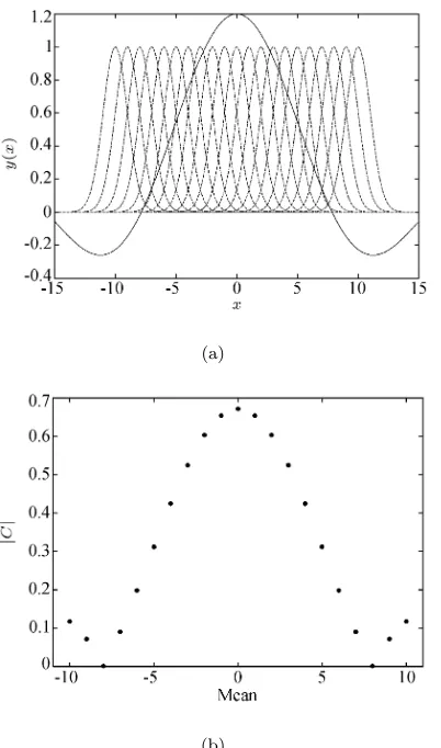
Fig. 1 (a) depicts the training data and the curves of the various Gaussian RBF units with different centres and a variance of 1.0, and Fig. 1 (b) shows the corre-sponding absolute correlation values between the train-ing data and Gaussian RBF regressors; while Fig. 1 (c) depicts the training data and the Gaussian RBF units with zero centre and various values of variance, and Fig. 1 (d) plots the corresponding values of the correla-tion between the training data and RBF regressors. For this example, |Ck(µk, σ2

k)| is maximised with µk = 0

andσ2k= 12.

(a)

(b)

(c)

(d)

Fig. 1 Illustration of RBF positioning and shaping using the correlation criterion: (a) the solid curve is the training

data set, and dashed curves are the Gaussian RBF units with different centres and a variance of 1.0, and (b) the

corresponding values of the correlation between the training data and RBF units; while (c) the solid curve is the training data set, and dashed curves are the Gaussian RBF units with zero centre and various values of variance,

and (d) the corresponding values of the correlation between the training data and RBF units

RBF weight calculation. After the determination of thekth regressorgk(x), the corresponding RBF weight

wk can be calculated by minimising the MSE for the

k-unit RBF model with respect towk

MSEk =

1

N N

X

i=1

y(k)i

2 =

1

N N

X

i=1

y(k−1)

i −wkgk(xi)

2

. (8)

This leads to the usual least squares solution

wk = PN

i=1y (k−1)

i gk(xi)

PN

i=1g2k(xi)

It can be shown that selecting RBF units by incre-mentally maximising|Ck(µk,Σk)|is identical to

incre-mentally minimising the modelling MSE (8). In fact, substituting (5) into (8) withwk given by (9) yields

MSEk=

1 N N X i=1

y(k−1)

i

2 !

1−Ck2(µk,Σk).

(10) Clearly maximising|Ck(µk,Σk)| is equivalent to

min-imising MSEk with respect toµ_k and Σk.

B. Incremental modelling to construct a RBF net-work

The proposed procedure for constructing a RBF network can now be summarised. Refer to the defi-nition of the MSE (8) for thek-term RBF model. Give a preset modelling accuracyξMSE, and setk= 0.

Do: k=k+ 1

1) Determine the mean vector µk and covariance

matrix Σk of the k-th RBF unit by maximising the

correlation criterion|Ck(µ_k,Σk)|

2) Calculate the model weightwkfor thek-th RBF unit according to (9) and compute the modelling errors

yi(k)=y (k−1)

i −wkgk(xi), 16i6N

WhileMSEk < ξMSE

The termination of the model construction process can alternatively be decided using cross validation[16,17]_{. A simple method is to have a separate}

validation data set. The model construction is based on the training data set, while the performance of the selected model, the MSE (8), is monitored over the vali-dation data set. The construction process is terminated when the MSE over the validation set stops improving. Alternatively, the Akaike information criteria[28,29]_and

the optimal experimental design criteria[6,30] _{can be}

employed to terminate the model construction proce-dure without the need to specify a modelling accuracy

ξMSE.

C. Repeated weighted boosting search optimisation

It can be seen that at thek-th stage of construction, the task is to minimise the cost function

J(u) = 1− |Ck(u)| (11)

where the parameter vectorucontains the centre vec-torµkand covariance matrixΣk of thek-th RBF unit.

This task may be carried out with a gradient based optimisation method[27]_{. A gradient method however}

depends on the initial condition and may be trapped at some bad local minima. Alternatively, the global optimisation methods, such as the GA[31,32] _and

adap-tive simulated annealing (ASA)[33,34], can be used. In this study, we employ a guided random search algo-rithm called the RWBS[26]_{to perform this optimisation}

task. The RWBS algorithm is a simple yet efficient

global search algorithm. In several global optimisation applications investigated in [26], the RWBS algorithm achieved a similar convergence speed as the GA and ASA. The RWBS algorithm has additional advantages of requiring minimum programming effort and having very few algorithmic parameters that require to tune, compared with the GA or ASA. The detailed RWBS algorithm for fitting the k-th RBF unit is now sum-marised.

Specify the population sizePS, the number of gen-erations in the repeated search NG, and the accuracy for terminating the weighted boosting searchξB.

Outer loop: generations Forl= 1 :NG Generation initialisation: Initialise the population by setting u(l)₁ =u(l_best−1) and randomly generating rest of the population members u(l)_i , 2 6 i 6 PS, where

u(l_best−1)denotes the solution found in the previous gen-eration. Ifl= 1,u(l)₁ is also randomly chosen

Weighted boosting search initialisation: Assign the initial distribution weightingsδi(0) = 1

PS, 16i6PS, for the population, and calculate the cost function value of each pointJi=J(u(l)_i ), 16i6PS

Inner loop: weighted boosting search Set

t= 0; Fort=t+ 1

Step 1: Boosting

1) Find

ibest= arg min

16i6PS

Ji and iworst= arg max

16i6PS

Ji

Denoteu(l)_best=u(l)_ibest andu(l)_worst=u(l)_iworst

2) Normalise the cost function values

¯

Ji = _PJi S

X

m=1 Jm

, 16i6PS

3) Compute a weighting factorβtaccording to

ηt=

PS

X

i=1

δi(t−1) ¯Ji, βt= ηt 1−ηt

4) Update the distribution weightings for 1 6i 6 PS

δi(t) = (

δi(t−1)βJ¯i

t , forβt61 δi(t−1)β1−J¯i

t , forβt>1

and normalise them

δi(t) = _Pδi(t) S

X

m=1 δm(t)

, 16i6PS

Step 2: Parameter updating

1) Construct the (PS+ 1)th point using the formula

uPS+1=

PS

X

i=1

2) Construct the (PS+ 2)th point using the formula

uPS+2=u

(l) best+

u(l)_best−uPS+1

3) Compute the cost function values Ji = J(ui), i=PS+ 1, PS+ 2, for these two points and find

i_∗= arg min

i=PS+1,PS+2

Ji

4) The pair (ui_∗, Ji_∗) then replaces (u(l)worst, Jiworst)

in the population

IfkuPS+1−uPS+2k< ξB, exitinner loop

End of inner loop

The solution found in the l-th generation is u =

u(l)_best

End of outer loop

This yields the solutionu=u(NG)

best , i.e. µk andΣk

of thek-th RBF unit.

The motivations and analysis of the RWBS algo-rithm as a global optimiser is detailed in [26]. To guar-antee a global optimal solution as well as to achieve a fast convergence, PS, NG and ξB need to be set carefully. The appropriate values for these algorith-mic parameters depend on the dimension ofuand how hard the objective function to be optimised, and gen-erally they have to be found empirically. The elitist initialisation is very useful, as it keeps the information obtained by the previous search generation, which oth-erwise would be lost due to the randomly sampling ini-tialisation. In the inner loop optimisation, there is no need for every members of the population to converge to a (local) minimum, and it is sufficient to locate where the minimum lies. Thus ξB can be set to a relatively large value. This makes the search efficient, achieving convergence with a small number of the cost function evaluations. A sufficiently largeNG should be used to ensure that the parameter space is sampled sufficiently.

3

Experimental results

Two simulated systems and two real-data sets were used to investigate the proposed RBF network con-struction method. Gaussian RBF units were used in all the examples. The RWBS algorithmic parameters,

PS, NG and ξB, were set empirically. We also as-sumed that the desired modelling accuracyξMSEcould be chosen. We point out that other automatic termina-tion criteria[6] _{can be adopted as alternatives without}

the need of specifying ξMSE. The standard SVM algo-rithm with the ε-insensitive loss function[9] _{was used}

as the benchmarker in the modelling experiments. The three learning parameters of theε-insensitive SVM al-gorithm, theεvalue and the value of the regularisation

parameterCas well as the RBF varianceσ2_{, were}

de-termined empirically via cross validation.

Example 1. The 500 points of training data were generated from

y(x) = 0.1x+sinx

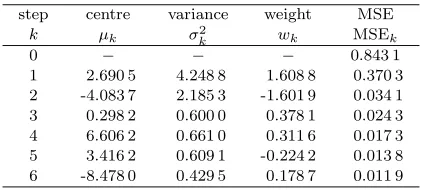
x + sin 0.5x+e (12)

with equally spaced x ∈ [−10, 10], where e was a Gaussian white noise with zero mean and variance 0.01. With the modelling accuracy set to ξMSE = 0.012, the proposed incremental RBF model construction proce-dure produced 6 Gaussian RBF units, as summarised in Table 1, and the construction process is also illus-trated graphically in Fig. 2. The model output of the constructed 6-unit RBF model is superimposed on the noisy training data in Fig. 3 (a), and the modelling er-rors are shown in Fig. 3 (b). The MSE of this RBF model was 0.011 9.

Table 1 Incremental construction of the RBF network for Example 1

step centre variance weight MSE

k µk σ_k2 wk MSEk

0 − − − 0.843 1

1 2.690 5 4.248 8 1.608 8 0.370 3 2 -4.083 7 2.185 3 -1.601 9 0.034 1 3 0.298 2 0.600 0 0.378 1 0.024 3 4 6.606 2 0.661 0 0.311 6 0.017 3 5 3.416 2 0.609 1 -0.224 2 0.013 8 6 -8.478 0 0.429 5 0.178 7 0.011 9

For theε-SVM algorithm, it was found thatσ2_{= 4,} ε= 0.245 andC = 10 was appropriate, and the algo-rithm selected 15 support vectors (SVs) with the MSE value of 0.012 6. The modelling performance of the resulting SVM model is shown in Fig. 4. The SVM algorithm achieves a similar modelling accuracy as the proposed incremental modelling method but it requires a much larger RBF network.

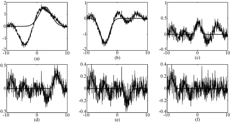
Fig. 2 Incremental construction of the RBF network for Example 1: in (a)–(f), the light curves are the modelling errors of the previous stage,y(k−1)

i , and the dark curves are the fitted current RBF units,wkgk(xi), for 16k66, respectively

(a) _(b)

Fig. 3 Incremental construction of the RBF network for Example 1: (a) the solid curve is the noisy training datayiand the dashed

curve is the constructed 6-unit RBF model ˆy, and (b) the modelling errore(xi) =yi−_yˆ(_xi)

(a) _(b)

Fig. 4 SVM construction of the RBF network for Example 1: (a) the solid curve is the noisy training datayi, the dashed curve is the

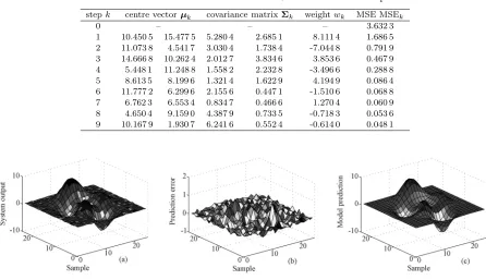
Table 2 Incremental construction of the RBF network for Example 2

stepk centre vectorµk covariance matrixΣk weightwk MSE MSEk

0 – – – 3.632 3

1 10.450 5 15.477 5 5.280 4 2.685 1 8.111 4 1.686 5 2 11.073 8 4.541 7 3.030 4 1.738 4 -7.044 8 0.791 9 3 14.666 8 10.262 4 2.012 7 3.834 6 3.853 6 0.467 9 4 5.448 1 11.248 8 1.558 2 2.232 8 -3.496 6 0.288 8 5 8.613 5 8.199 6 1.321 4 1.622 9 4.194 9 0.086 4 6 11.777 2 6.299 6 2.155 6 0.447 1 -1.510 6 0.068 8 7 6.762 3 6.553 4 0.834 7 0.466 6 1.270 4 0.060 9 8 4.650 4 9.159 0 4.387 9 0.733 5 -0.718 3 0.053 6 9 10.167 9 1.930 7 6.241 6 0.552 4 -0.614 0 0.048 1

Fig. 5 Incremental construction of the RBF network for Example 2: (a) the noisy training data, (b) the modelling errors for the constructed 9-unit RBF model, and (c) the model outputs of the constructed 9-unit RBF model

For the SVM modelling, σ2 = 4, ε = 0.45 and

C = 10 were found to be appropriate, and the algo-rithm constructed a RBF model with a MSE value of 0.047 1, which is similar to the MSE of the 9-unit RBF model constructed by the proposed algorithm. How-ever, the constructed SVM model contained 42 SVs. The size of this SVM model is therefore more than four times of that produced by the proposed sparse construction algorithm. The modelling performance of this 42-unit RBF model is depicted in Fig. 6.

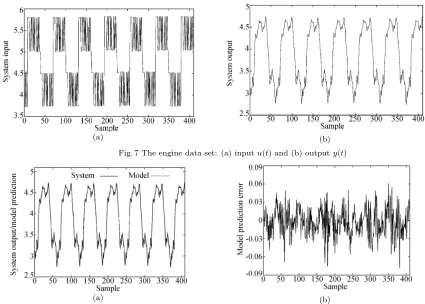
Example 3. This example modelled the relation-ship between the fuel rack position (inputu(t)) and the engine speed (output y(t)) for a turbocharged, direct injection diesel engine operated at low engine speed. Detailed system description and experimental setup can be found in [35]. The data set, depicted in Fig. 7, contained 410 samples. The first 210 data points were used in training and the last 200 points in model vali-dation. The previous study[6]_{has shown that this data}

set can be modelled adequately asyi=F(xi) +eiwith yi =y(i),xi= [y(i−1)u(i−1)u(i−2)]T, whereF(•)

describes the underlying system to be identified andei

denotes the system noise. With the modelling accuracy of ξMSE = 0.000 55, the proposed construction proce-dure produced 9 Gaussian RBF units, and the resulting model is listed in Table 3. The MSE values of this 9-unit RBF model over the training and testing sets were

0.000 532 and 0.000 558, respectively. Fig. 8 depicts the modelling performance for this 9-unit RBF model.

Using a cross validation, it was found that σ2 ₌

1.69, ε = 0.02 and C = 4 were appropriate for the SVM algorithm, and the algorithm produced a RBF network with 89 SVs. The MSE values for this 89-unit RBF model were 0.000 495 and 0.000 524 over the training and test sets, respectively. Fig. 9 shows the modelling performance of this 89-unit RBF model. It can be seen that the proposed sparse construction al-gorithm is capable of producing a much sparser RBF network with the same excellent generalisation perfor-mance, in comparison with the SVM algorithm.

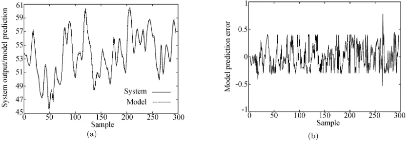
Example 4. This example constructed a model for the gas furnace data set (Series J in [36]). The data set contained 296 pairs of input-output points, where the input u(t) was the coded input gas feed rate and the output y(t) represented CO2 concentration from

the gas furnace. The input-output data are depicted in Fig. 10. The training data set was constructed with

yi=y(i) andxi= [y(i−1)y(i−2)y(i−3)u(i−1)u(i−

(a) _(b)

Fig. 6 SVM construction of the RBF network for Example 2: (a) the modelling errors for the constructed 42-unit RBF model, and (c) the model outputs of the constructed 42-unit RBF model

(a) _(b)

Fig. 7 The engine data set: (a) inputu(t) and (b) outputy(t)

(a) _(b)

Fig. 8 Incremental construction of the RBF network for Example 3, the engine data set: (a) model prediction ˆy(t) (dashed) superimposed on system outputy(t) (solid), and (b) model prediction errore(t) =y(t)−_yˆ(_t). The proposed sparse construction

procedure constructed a 9-unit RBF model

Table 3 Incremental construction of the RBF network for Example 3, the engine data set

stepk centre vectorµk covariance matrixΣk weightwk MSE MSEk×100

0 – – – 1 558.9

(a) _(b)

Fig. 9 SVM construction of the RBF network for Example 3, the engine data set: (a) model prediction ˆy(t) (dashed) superimposed on system outputy(t) (solid), and (b) model prediction errore(t) =y(t)−ˆ_y(_t). The SVM algorithm constructed a 89-unit RBF model

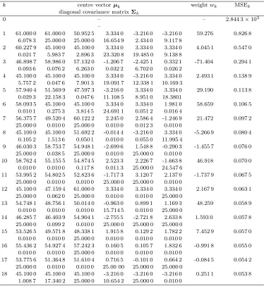
Table 4 Incremental construction of the RBF network for Example 4, the gas furnace data set

k centre vectorµk weightwk MSEk

diagonal covariance matrixΣk

0 – – 2.844 3×103

–

1 61.000 0 61.000 0 50.952 5 3.334 0 -3.216 0 -3.216 0 59.276 0.826 8 6.078 3 25.000 0 25.000 0 16.654 9 2.434 0 9.117 8

2 60.227 9 45.100 0 45.100 0 3.334 0 3.334 0 3.334 0 4.045 1 0.547 0 0.021 7 5.983 7 2.896 3 23.320 8 19.485 0 9.138 8

3 46.898 7 58.986 0 57.132 0 -1.206 7 -2.425 1 0.332 1 -71.404 0.294 1 0.093 6 0.076 2 6.263 0 0.032 2 6.702 0 0.026 2

4 45.100 0 45.100 0 45.100 0 3.334 0 -3.216 0 3.334 0 2.493 1 0.138 9 5.757 2 0.047 6 7.901 3 19.091 7 12.338 1 10.169 3

5 57.940 4 51.569 9 47.597 3 -3.216 0 3.334 0 3.334 0 29.190 0.113 8 0.029 3 22.158 3 0.047 6 11.108 5 8.951 0 18.3801

6 58.093 5 45.100 0 45.100 0 3.334 0 3.334 0 1.981 0 58.659 0.106 5 0.010 1 0.275 3 3.814 5 24.691 1 0.051 2 0.016 4

7 56.375 7 49.520 4 60.122 2 2.245 0 2.586 4 -1.246 9 21.472 0.097 2 25.000 0 0.010 0 25.000 0 0.010 0 0.012 3 0.010 0

8 45.100 0 45.100 0 51.692 2 -0.014 4 -3.216 0 3.334 0 -5.266 9 0.080 4 0.105 2 1.513 6 0.050 1 0.010 0 0.055 0 11.995 4

9 46.030 3 58.753 7 54.948 1 -2.699 6 1.548 8 -0.290 3 -1.455 7 0.076 0 25.000 0 0.038 5 25.000 0 0.010 0 25.000 0 0.010 0

10 58.762 4 55.155 5 54.874 5 2.523 3 2.226 7 -1.663 8 46.918 0.070 0 0.010 0 0.010 0 0.117 8 0.011 3 25.000 0 24.547 6

11 53.995 2 54.802 5 52.823 6 -1.717 3 3.120 7 2.137 0 -1.737 9 0.067 5 25.000 0 0.010 0 0.010 0 25.000 0 25.000 0 0.010 0

12 45.100 0 47.159 4 61.000 0 3.334 0 3.334 0 3.334 0 2.167 9 0.063 1 25.000 0 0.062 0 25.000 0 0.010 0 0.010 0 25.000 0

13 54.748 1 48.756 1 50.014 0 -0.963 0 0.899 1 1.169 3 48.259 0.058 9 0.010 0 0.010 0 0.010 0 15.714 5 0.010 0 25.000 0

14 46.285 7 46.403 9 54.904 1 -2.755 5 -2.721 8 2.633 8 1.593 0 0.057 8 25.000 0 0.099 2 0.010 0 25.000 0 25.000 0 25.000 0

15 53.526 5 49.571 8 48.338 1 1.915 8 0.129 2 1.782 2 7.452 9 0.057 0 0.010 0 0.010 0 25.000 0 0.010 0 0.010 0 0.010 0

16 55.436 2 54.927 4 57.242 3 0.160 5 0.105 7 1.832 6 -0.991 8 0.055 0 0.010 0 0.010 0 25.000 0 0.010 0 0.010 0 0.010 0

17 53.775 6 51.364 8 51.610 4 0.716 5 -0.101 0 0.664 2 -0.084 5 0.054 2 25.000 0 0.010 0 0.010 0 25.00 00 25.000 0 25.000 0

(a) _(b) Fig. 10 The gas furnace data set: (a) inputu(t) and (b) outputy(t)

(a) _(b)

Fig. 11 Incremental construction of the RBF network for Example 4, the gas furnace data set: (a) model prediction ˆy(t) (dashed) superimposed on system outputy(t) (solid), and (b) model prediction errore(t) =y(t)−_yˆ(_t). The proposed sparse construction

procedure constructed a 18-unit RBF model

(a) _(b)

Fig. 12 SVM construction of the RBF network for Example 4, the gas furnace data set: (a) model prediction ˆy(t) (dashed) superimposed on system outputy(t) (solid), and (b) model prediction errore(t) =y(t)−_yˆ(_t). The SVM algorithm constructed a

61-unit RBF model

Next, the SVM algorithm was applied to this ex-ample. The appropriate values for the SVM’s learning parameters were found to be σ2 _{= 20, ε = 0.35 and} C = 300. The RBF model constructed by the SVM algorithm contained 61 SVs with the modelling MSE value of 0.052 0. Fig. 12 depicts the modelling

4

Conclusions

A novel technique has been presented to construct sparse RBF network models for regression. Unlike most of the sparse kernel regression methods, which restrict RBF centres to the training input data and use a fixed common variance for all the RBF units, the proposed technique can tune the centre vector and diagonal co-variance matrix of individual RBF unit to best fit the training data based on the correlation between the RBF regressor and the training data. This technique thus provides enhanced modelling capability. An effi-cient repeated weighted boosting search optimisation method has been employed based on the correlation criterion to append RBF units one by one in an in-cremental construction procedure. Using the standard SVM method as the benchmarker, experiments have been conducted using several regression modelling ex-amples, and it has been shown that the proposed RBF network construction method is capable of producing much sparser model representations with the same ex-cellent generalisation performance in comparison with the SVM algorithm.

References

[1] S. Chen, S. A. Billings, W. Luo. Orthogonal Least Squares Methods and Their Application to Non-Linear System Iden-tification. International Journal of Control, vol. 50, no. 5, pp. 1873−1896, 1989.

[2] S. Chen, C. F. N. Cowan, P. M. Grant. Orthogonal Least Squares Learning Algorithm for Radial Basis Function Net-works. IEEE Transactions on Neural Networks, vol. 2, no. 2, pp. 302−309, 1991.

[3] M. J. L. Orr. Regularization in the Selection of Radial Basis Function Centres. Neural Computation, vol. 7, no. 3, pp. 606−623, 1995.

[4] S. Chen, E. S. Chng, K. Alkadhimi. Regularised Orthogo-nal Least Squares Algorithm for Constructing Radial Basis Function Networks. International Journal of Control, vol. 64, no. 5, pp. 829−_{837, 1996.}

[5] S. Chen, Y. Wu, B. L. Luk. Combined Genetic Algorithm Optimisation and Regularised Orthogonal Least Squares Learning for Radial Basis Function Networks. IEEE Trans-actions on Neural Networks, vol. 10, no. 5, pp. 1239−1243,

1999.

[6] S. Chen, X. Hong, C. J. Harris. Sparse Kernel Regression Modelling Using Combined Locally Regularized Orthogo-nal Least Squares and D-Optimality Experimental Design.

IEEE Transactions on Automatic Control, vol. 48, no. 6, pp. 1029−1036, 2003.

[7] S. Chen, X. Hong, C. J. Harris, P. M. Sharkey. Sparse Mod-elling Using Orthogonal Forward Regression with PRESS Statistic and Regularization.IEEE Transactions on Systems, Man and Cybernetics, Part B, vol. 34, no. 2, pp. 898−911,

2004.

[8] V. Vapnik. The Nature of Statistical Learning Theory. Springer-Verlag, New York, 1995.

[9] S. Gunn. Support Vector Machines for Classification and Re-gression. Technical Report, Information: Signals, Images, Systerms (ISIS) Research Group, Department of Electron-ics and Computer Science, University of Southampton, UK, May 1998.

[10] S. S. Chen, D. L. Donoho, M. A. Saunders. Atomic Decom-position by Basis Pursuit. SIAM Review, vol. 43, no. 1, pp. 129−159, 2001.

[11] M. E. Tipping. Sparse Bayesian Learning and the Relevance Vector Machine. Journal of Machine Learning Research, vol. 1, pp. 211−244, 2001.

[12] B. Sch¨olkopf, A. J. Smola. Learning with Kernels: Support Vector Machines, Regularization, Optimization, and Beyond. MIT Press, Cambridge, MA, 2002.

[13] P. Vincent, Y. Bengio. Kernel Matching Pursuit. Machine Learning, vol. 48, no. 1, pp. 165−187, 2002.

[14] G. R. G. Lanckriet, N. Cristianini, P. Bartlett, L. E Ghaoui, M. I. Jordan. Learning the Kernel Matrix with Semidefinite Programming. Journal of Machine Learning Research, vol. 5, pp. 27−72, 2004.

[15] T. Doddy. Priori Knowledge for Time Series Modeling. Ph.D These, Department of Electronics and Computer Sci-ence, University of Southampton, U.K., 2000.

[16] M. Stone. Cross Validation Choice and Assessment of Statis-tical Predictions. Journal of Royal Statistics Society, Series B, vol. 36, pp. 117−147, 1974.

[17] R. H. Myers. Classical and Modern Regression with Appli-cations. 2nd ed., PWS-KENT, Boston, 1990.

[18] S. Lee, R. M. Kil. A Gaussian Potential Function Network with Hierarchically Self-Organizing Learning. Neural Net-works, vol. 4, no. 2, pp. 207−_{224, 1991.}

[19] S. Chen, X. Hong, C. J. Harris, X. X. Wang. Identification of Nonlinear Systems Using Generalized Kernel Models. IEEE Transactions on Control Systems Technology, vol. 13, no. 3, pp. 401−411, 2005.

[20] G. B. Huang, P. Saratchandran, N. Sundararajan. A Gen-eralized Growing and Pruning RBF (GGAP-RBF) Neural Network for Function Approximation. IEEE Transactions on Neural Networks, vol. 16, no. 1, pp. 57−67, 2005.

[21] J. Moody, C. J. Darken. Fast Learning in Networks of Locally-Tuned Processing Units. Neural Computation, vol. 1, pp. 281−294, 1989.

[22] S. Chen, S. A. Billings, P. M. Grant. Recursive Hybrid Al-gorithm for Non-Linear System Identification Using Radial Basis Function Networks. International Journal of Control, vol. 55, pp. 1051−1070, 1992.

[23] S. Chen. Nonlinear Time Series Modelling and Prediction Using Gaussian RBF Networks with Enhanced Clustering and RLS Learning. Electronics Letters, vol. 31, no. 2, pp. 117−_{118, 1995.}

[24] P. E. An, M. Brown, S. Chen, C. J. Harris. Comparative As-pects of Neural Network Algorithms for On-Line Modelling of Dynamic Processes. InProceedings of the Institution of Mechanical Engineers, Part I, Journal of Systems and Con-trol Engineering, vol. 207, pp. 223−241, 1993.

[25] B. A. Whitehead, T. D. Choate. Evolving Space-Filling Curves to Distribute Radial Basis Functions Over an Input Space. IEEE Transactions on Neural Networks, vol. 5, no. 1, pp. 15−23, 1994.

[26] S. Chen, X. X. Wang, C. J. Harris. Experiments with Re-peating Weighted Boosting Search for Optimization in Sig-nal Processing Applications. IEEE Transactions on Systems, Man and Cybernetics, Part B, vol. 35, no. 4, pp. 682−693,

2005.

[27] S. E. Fahlman, C. Lebiere. The Cascade-Correlation Learn-ing Architecture. Neural Information Processing Systems 2, D.S. Touretzky, Ed., Morgan-Kaufmann, San Fransisco, CA, pp. 524−532, 1990.

[28] H. Akaike. A New Look at the Statistical Model Identifica-tion. IEEE Transactions on Automatic Control, vol. AC-19, pp.716−723, 1974.

of Control, vol. 45, no. 1, pp. 311−341, 1987.

[30] X. Hong, C. J. Harris. Nonlinear Model Structure Design and Construction Using Orthogonal Least Squares and D-Optimality Design.IEEE Transactions on Neural Networks, vol. 13, no. 5, pp. 1245−1250, 2002.

[31] D. E. Goldberg. Genetic Algorithms in Search, Optimiza-tion and Machine Learning. Addison Wesley, Reading, MA, 1989.

[32] K. F. Man, K. S. Tang, S. Kwong. Genetic Algorithms: Concepts and Design. Springer-Verlag, London, 1998. [33] L. Ingber. Simulated Annealing: Practice Versus Theory.

Mathematical and Computer Modeling, vol. 18, no. 11, pp. 29−57, 1993.

[34] S. Chen, B. L. Luk. Adaptive Simulated Annealing for Opti-mization in Signal Processing Applications. Signal Process-ing, vol. 79, no. 1, pp. 117−128, 1999.

[35] S. A. Billings, S. Chen, R. J. Backhouse. The Identifica-tion of Linear and Non-Linear Models of a Turbocharged Automotive Diesel Engine. Mechanical Systems and Signal Processing, vol. 3, no. 2, pp. 123−142, 1989.

[36] G. E. P. Box, G. M. Jenkins. Time Series Analysis, Fore-casting and Control. Holden Day Inc., 1976.

Xun-xian Wang received his Ph.D. degree in the control theory and appli-cation field from Tsinghua University, Beijing, China, in July 1999.

From August 1999 to August 2001, he was a postdoctoral researcher in the State Key Laboratory of Intelli-gent Technology and Systems, Beijing, China. From September 2001 to De-cember 2004, he was a research fellow at the University of Portsmouth, Port-smouth, U.K. From January 2005, he has been a research fellow at Neural Computing Research Group, Aston University, Birm-ingham, U.K.

His main research interests include machine learning and neural networks, control theory and systems as well as robot-ics.

Sheng Chen received his Ph.D. de-gree in control engineering from the City University, London, U.K., in 1986. He joined the School of Electron-ics and Computer Science, University of Southampton, Southampton, U.K., in September 1999. He previously held research and academic appointments at the University of Sheffield, the Uni-versity of Edinburgh, and the Univer-sity of Portsmouth, all in U.K.

He has published over 260 research papers. His research works include wireless communications, machine learning and neural networks, finite-precision digital controller design, and evolutionary computation methods.

Professor Chen holds a higher doctorate degree, D.Sc, from the University of Southampton. In the database of the world’s most highly cited researchers, compiled by Institute for Scien-tific Information (ISI) of the USA, Dr. Chen is on the list of the highly cited researchers in the engineering category.

Chris Harrisreceived his Ph.D. de-gree from the University of Southamp-ton, SouthampSouthamp-ton, U.K.

He previously held appointments at the University of Hull, the UMIST, the University of Oxford, and the Univer-sity of Cranfield, all in U.K., as well as being employed by the U.K. Ministry of Defence. He returned to the Univer-sity of Southampton as the Lucas Pro-fessor of Aerospace Systems Engineer-ing in 1987 to establish the Advanced Systems Research Group and, more recently, Image, Speech and Intelligent Systems Group.

He has authored and co-authored 12 research books and over 400 research papers, and he is the associate editor of numerous international journals. His research interests include the general area of intelligent and adaptive systems theory and its applica-tion to intelligent autonomous systems such as autonomous ve-hicles, management infrastructures such as command & control, intelligent control, and estimation of dynamic processes, multi-sensor data fusion, and systems integration.