Plasma drift waves and instabilities

PLASMA DRIFT WAVES AND INSTABILITIES

William Allan

A Thesis Submitted for the Degree of PhD

at the

University of St Andrews

1974

Full metadata for this item is available in

St Andrews Research Repository

at:

http://research-repository.st-andrews.ac.uk/

Please use this identifier to cite or link to this item:

http://hdl.handle.net/10023/14011

PLASMA' DRIFT WAVES AND

INSTABILITIES

William. Allan

Thesis submitted for the Degree of Doctor of Philosophy of the University of St, Andrews

ProQuest Number: 10167144

All rights reserved

INFORMATION TO ALL USERS

The quality of this reproduction is dependent upon the quality of the copy submitted.

In the unlikely event that the author did not send a com plete manuscript and there are missing pages, these will be noted. Also, if material had to be removed,

a note will indicate the deletion.

uest

ProQuest 10167144

Published by ProQuest LLO (2017). Copyright of the Dissertation is held by the Author.

All rights reserved.

This work is protected against unauthorized copying under Title 17, United States C ode Microform Edition © ProQuest LLO.

ProQuest LLO.

789 East Eisenhower Parkway P.Q. Box 1346

ABSTRACT

The work of this thesis is concerned with the investigation of the propagation of waves in a magnetized plasma containing various parameter gradients, and with the stability of ion acoustic waves in a weakly collisional plasma with a strong temperature gradient.

The thesis is divided into three sections. In the first section the intention is to derive in a compact and unambiguous tensor form the dispersion relation describing the propagation of waves in a magnetized plasma containing three-dimensional density and temperature gradients, an E A B drift, and differing temperatures parallel and perpendicular to the magnetic field. This is achieved by introducing and extending the polarized co-ordinate system first proposed by Buneman in I9 6I, and then carrying through the standard procedure of integration along

unperturbed trajectories. The "local" approximation of Krall and Rosenbluth is used in order that an analytic result may be derived. The dispersion relation obtained includes certain moment tensors whose elements may be evaluated independently of the gradients involved in the problem. These elements may then be listed and the list referred to in order to obtain the elements required for a specific problem.

The second section is concerned with the use of the theory and results of J.P. Dougherty to show that in the high-frequency regime the introduction of a small amount of collisions into a plasma is sufficient to disrupt the gyro-resonances which allow the existence of Bernstein waves at multiples of the gyro-frequencies perpendicular and near- perpendicular to the magnetic field. It is shown that a collision

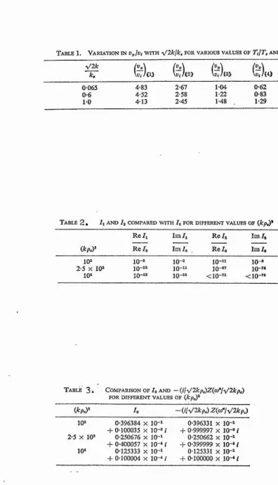
frequency v such that (kp)”^ < ~ < (kp)""^ where kp >> 1 is sufficient to do this; k is the wave-number, p the Larmor radius, and U _the

gyro-frequency. It is also shown that in this case the ion-acoustic dispersion relation is valid even for propagation perpendicular to the magnetic field.

In the final section the result of the second section is used to derive a dispersion relation for high-frequency wave propagation in a weakly-collisional plasma containing an electron temperature gradient. The dispersion relation is solved numerically for various electron-ion temperature ratios and electron temperature gradient drift velocities. Earlier predictions, based on analytic calculations for small temperature ratios and drift velocities, are confirmed and some new results presented. In particular, it is shown that a temperature gradient is a more effective destabilizing agent then a simple drift between ions and electrons.

Dispersion plots are given, along with analytic and physical explanations of their form; finally neutral stability curves are presented.

DECLARATION

POSTGRADUATE CAREER

I

I

student under Ordinance General No. 12 in October 1971, to carry out -r-research work into the theory of waves in magnetized plasmas under

CERTIFICATE

ACKNOWLEDGEMENTS

I extend my heartfelt appreciation to my Supervisor, Dr. J.J. Sanderson, for his help, encouragement and endless patience throughout the preparation of the work presented in this thesis. I would like to thank Mr. T.J. Martin and Dr. C.N. Lashmore-Davies of Culham Laboratory, and Dr. R.A. Cairns of St. Andrews University, for their assistance and helpful suggestions. I would also like to thank Mrs. Margaret Sweeney for her dedication and accuracy in carrying through the typing of this thesis.

CONTENTS

INTRODUCTION :

Page

SECTION I A dispersion relation for a plasma with various spatial inhomogeneities.

Chapter 1 : 8

Chapter 2 : 1^

Chapter 3 : 2U

SECTION II The effect of weak collisions on the Bernstein modes.

Chapter 1 ; 31

Chapter 2 : 36

Chapter 3 : ^0

Chapter U : 52

SECTION III Temperature gradient driven ion acoustic instability.

Chapter 1 : 59

Chapter 2 ; 62

Chapter 3 : 69

REFERENCES : 127

3

I

SUMMARY OF RESULTS : 76

1

APPENDIX I : 78

APPENDIX II : 86

APPENDIX III : 95 "t

APPENDIX IV : 108 Âi

%

TABLES nU _i

,|

-1 —

INTRODUCTION |

Plasma physics is a young science. The use of the term "plasma" ' to describe a partly or wholly ionized gas is not yet half-a-century old; yet plasma physics is the apex of a pyramid of scientific thought and * experiment. Just below the apex lie the ideas of Vlasov and Landau,

Alfven, Tonks and Langrauir, Appleton and Hartree; deepening and

I

broadening the pyramid beneath are the minds of Debye and Larmor, Maxwell %, and Boltzmann, Faraday, Gauss, Ampere, Volta... At the base of

the pyramid lies the foundation upon which the whole structure is built:- | I the minds of the Greek philosophers, in which the generic ideas of logical thought and theoretical science were born. Plasma physics may be young,

but it has a pedigree that cannot be bettered. f

In any fully-ionized plasma there are short-range interactions between a charged test-particle and individual particles close to it; there is also a long-range collective interaction between the test-particle and the averaged electromagnetic field of all the other particles in the plasma (or at least of all the other particles within the Debye sphere of the test-particle, where the radius of the Debye sphere is of order

k T

Htt Uq e^ ^ , K being Boltzmann's constant, T the mean temperature.

'I iIq the particle number density, and -e the electron charge). Short-range interactions have the effect of changing the trajectory of the test-particle over a relatively short time-scale, while the effect of the averaged

Coulomb field is experienced over a much longer time-scale. The collective ;■ interaction may be pictured as a smooth, gradual change in the trajectory

of the test-particle, with the short-range interactions as a series of

small but finite deviations superimposed on the slow collective change. ,| Depending on the density and temperature of the plasma, one or other 9 of these effects may dominate. If short-range interactions are so important that the collective interaction can be neglected, the plasma is termed a

~2~

"collision-dominated" plasma; it may be described by a model which considers local values of quantities such as mass density, net flow velocity, mean temperature and so on. This is justified because the test-particle is only affected by particles adjacent to it, and has no significant interaction with particles at a large distance. In essence, this description treats the plasma as a continuous fluid whose properties are averaged over a volume large enough to justify neglect of individual particle motions.

In the limiting case where short-range interactions may be neglected when compared with the collective interaction, the plasma is termed a

"collisionless" plasma. Fluid descriptions break down here since they are dependent on collision dominance; however in the so-called "cold- plasma" regime (where the coherent flow velocity of the plasma is much greater than the random thermal velocities of the constituent particles) a quasi-fluid description is possible, although the cold-plasma model is highly idealized.

Models of the plasma state have been developed from the basic idea of an infinite, homogeneous, isotropic, fully-ionized, collisionless

plasma with non-zero kinetic temperature. Simple and unrealistic as this may seem, the basic state is still capable of supporting a bewildering variety of waves and disturbances. These may be characterized by

deriving a dispersion relation for the plasma. This relation takes the following form:-.

D(w, k, p^, p^, p^ ) = 0

where w is the wave frequency

-1 k is the wave number, that is (wavelength)

-3-For example, consider the relation

üj^ = 0) ^ + k^c^_pe

2 _ nr

where w _pe - _m^

and o)pg is known as the electron plasma frequency, m is the electron mass,

c is the speed of light in vacuo.

This relation describes the propagation of transverse (or electromagnetic) waves in our basic plasma with zero kinetic temperature.

Situations may arise in a plasma in which the effects of collisions do not dominate the collective interaction mentioned earlier, and yet in which they cannot be neglected entirely. By their random nature,

collisions tend to disrupt coherent effects that may take place in a plasma; for instance the dispersion relation for a completely collisionless plasma may contain a resonance occurring at some particular frequency, giving rise to a propagating wave mode. The presence of even a very small amount of collisions may be sufficient to randomize the resonance so that the mode is destroyed; and collisions are always present in any real plasma.

Neither the fluid description nor the cold plasma model is equipped to deal with such a situation. Moreover, both of these descriptions contain averaging processes which lose many properties of the plasma; it is therefore of great interest to investigate a plasma in terms of kinetic theory. This is a more fundamental description than anything discussed

so far, in that it tries to deal with the microscopic particle nature of the plasma rather than considering averaged microscopic properties.

The use of kinetic theory, along with the introduction of applied electromagnetic fields, spatial gradients in density, temperature,

magnetic field and so forth, results in a much more realistic model, but also in a greatly Increased complexity of the dispersion relation.

M.

at

and to the long-range collective interaction, while _{at c} is the rate

3^ I 5 giving

of change of f due to microscopic interactions between particles, that is due to collisions. Detailed derivations of this equation are given in many works, for example in reference [ 1 ] ,

A collisionless plasma is described by the Vlasov equation [ 2 ] , or f af

collisionless kinetic equation, which neglects the term

■ »

- m ~

This may be linearized by setting f = f^ + f^ and F = F^ + F^, where f^ and Fq are equilibrium values, f^ and F^ being small perturbations.

Substituting these in the Vlasov equation and neglecting products of small quantities, the linearized Vlasov equation is obtained:-

3fl F„ Fj

at ar m ay m ay

Landau [3 ] solved this using Fourier-Laplace transforms; an expression for the electric field E was then obtained from f, . In principle, this

- 1

expression may be written in terms of transforms as

1

— Ij.—"

of a plasma particle species, denoted by f(r, y, t). This quantity is such that the product f ^ ^ gives the probable number of particles to be found within an increment dr of the point with position vector r while travelling with a velocity within an increment dv of the velocity

V at time t. The six-dimensional space including all points with co-ordinates (r, y) is called phase space. The dynamics of a particle species in phase space is normally described by the collisional kinetic

equation |

E(r,t) = k

-5-E(k,p)e^(-'- "

V

E(k,t)e^-‘- dk where E(k,t) = | E(k,p)e dp

Now E(k;p) has poles p.(k) with residues _J R.(k), where p.’ is in general

3 3

complex, say Pj = + iy^. Therefore, using Cauchy's Residue Theorem

V

E(k,t) = Z R. e ^ 3

-iw.t + Y.t e

3 3

The Maxwellian distribution function is defined as r2

’M ” ^0 m

3/2 r

2ïïkT exp mv'=2kT

This distribution describes a homogeneous, isotropic plasma species in thermal equilibrium. Using the Maxwellian as his f^ , Landau found that Yj < 0, and so E(k,t) decays as t tends to infinity, since a negative exponential factor is included in it. Any other plasma parameter that can be derived from f^ decays in a similar manner. Now Yj > 0 for any j would imply unlimited wave growth, or instability. Thus waves propagating

in a Maxwellian plasma are stable. The decay phenomenon described above is known as Landau damping.

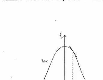
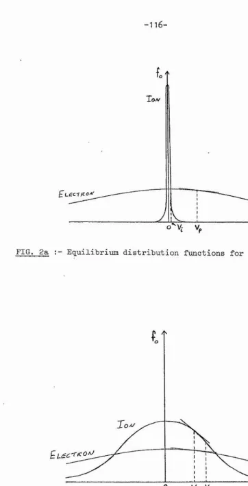
A physical explanation for this effect can be obtained by examining the distribution functions shown in Figure (la). For a wave with phase velocity v^, the number of particles of a given species travelling

slightly slower than the wave is greater than the number travelling

I

—6“

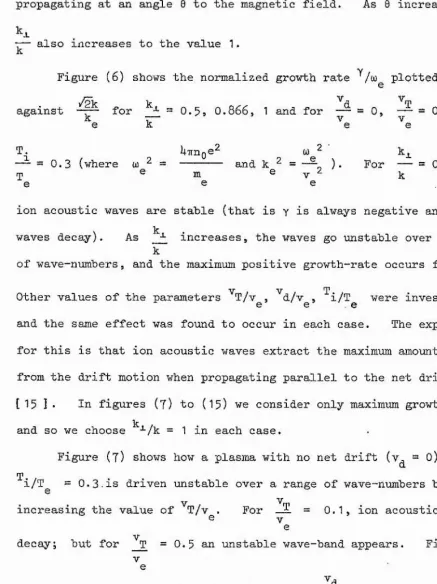
occurs for waves of all phase velocities. ° |

V, _d V, ₁would be necessary to cause instability (note that v. -_{1 ,e} kT i,e

“i,e

T . . T .

Thus plasmas that are unstable when i << 1 tend to stabilize as __i $

T T

*e e

increases.

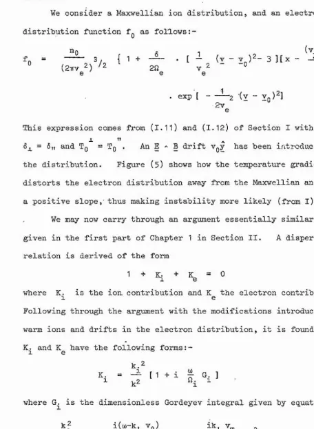
If a net drift velocity v^ of the electrons relative to the ions exists, the electron distribution is shifted in the positive v-direction as shown in Figure (lb). The part of the electron distribution from

V = 0 to V = v^ has positive slope. An isolated positive slope could

result in inverse Landau damping, so that waves might extract energy ■ I

'S from the electrons, and their amplitude would then grow. A negative ion J₃ slope also exists, however; growth occurs where the effect of the

positive electron slope is enough to overcome the effect of the negative ion slope. Thus instability occurs if v^ is large enough. Drifts and distortions of the distribution functions occur when the plasma contains applied electric and magnetic fields, and when there are spatial gradients in temperature, density, etcetera. Under these conditions the chance of instability occurring is greatly increased.

Differing ion and electron temperatures have an effect on plasma stability in the following way:- Consider Figure (2a) where T^ << T^ ; the ion gradient is very steep and negative for small positive v, and becomes negligible as v increases. This leaves only the weaker electron damping, so that a small electron drift can cause instability. Figure (2b) shows the distribution functions for T^ _ T^. The electron gradient is small for phase velocities near zero, but the ion gradient is steep enough to cause significant damping. The ion distribution also has enough spread to cause considerable damping for v^ _ v^, where the ion thermal velocity v. is no longer very small. Thus an electron drift of at least

7

-The study of all types of instability has become of the first ~| priority in recent years, since it was realized that most of the troubles

1

.ft another from plasma instabilities. In the first section of this thesis J we consider a collisionless plasma with various general particle drifts,

and derive a dispersion relation to describe the possible wave modes that 4 may propagate in it. In the second section we investigate one of the | cases mentioned earlier, in which the existence of a small collision | effect (in magnitude much less than the collective effect) is sufficient 4 to disrupt a resonance leading in the collisionless theory to a set of | propagating wave modes, the Bernstein modes. In the third section we ^ investigate in detail the effect of a large temperature gradient drift i on the wave-mode known as the ion acoustic wave in a thermal plasma |

including weak collisions. 4

We may note here that the method we use to solve the linearized j Vlasov equation is equivalent to Landau's Fourier-Laplace transform

1

method, and results in a four-fold integral over three velocity components 4 and time. If the time integral is performed first, followed by the i velocity integrals, a solution may be obtained in terms of Bessel functions. 4 If the velocity integrals are performed first, a time integral known as 4 f; the Gordeyev integral (or some modification of it) is involved in the result. 5 For a general problem the former approach is usually the most profitable. 4 However for a more particular problem, perhaps concerning a simple S configuration or a limited parameter range, the Gordeyev integral approach is often to be preferred. For the general drift problem in Section I we

use the Bessel function approach; in Sections II and III the Gordeyev | (v, )

integral approach is used in the regime kp >> 1, where p ==• 'i’j. k

“ ■■

I

is the Larmor radius, and Cv_) is the mean thermal velocity perpendicular

I

ciB 3

to the magnetic field B. The cyclotron frequency 0 is ^ where

SECTION I : A dispersion relation for a plasma with various spatial inhomogeneities.

Chapter 1

In this section we derive a dispersion relation for a fully- ionized, collisionless, non-relativistic plasma which includes general gradients in density and temperature, and also differing temperatures parallel and perpendicular to an applied magnetic field.

The kinetic equation describing a particle species in such a plasma is the collisionless kinetic equation, or Vlasov equation

3f

df ^ _{3f F}

at - ' ar g 3v -s= 0 (1.1)

In this equation r and v denote position and velocity respectively, so that (r,v) is a position in phase space. The species distribution

function is f(r,v,t), while F represents the net macroscopic force acting on a particle of the species. This force includes the effect of external forces and of the internal averaged collective force due to particles of all species, but excludes microscopic short-range particle collisions. The particle mass in represented by m.

To solve (l.l) in the linear theory, we must examine the effect of small perturbations on a plasma which is initially in an equilibrium state We therefore make the following

substitution:-:^(Y)Y)t) = fQ(r,y) + f^(r,y,t) F(r,v,t) = Fq(r,v) + Ei (^jVs't)

where f^ and F^ are equilibrium values, and f^ and F^ are small perturbations such that

< < 1 and

Using this, equation (l.l) becomes

-9-Sfo afo Eo 3fo

^ 9t * - ' 9r ^ râ~ * 9v

;|

9 fl 9 fi Fo 9 fi

h

+ [ TT— + V . T--+ . ]

El af

+ Y .---T~-- + --- .-- T-- - - • %--- (1.3)

9t - 9r m 9v m 9v

The solution of this equation, fi(psV,t), contains in principle all the information required to describe the perturbed plasma.

Equation (1.3) may be written in the following

form:-[ • ^ ] fi = h(r,y,t)

where h(r,v,t) = _m Ei _9v

and E _{dt ^}1 is a differential operator acting along the characteristic

9t - * 9r m ' 9v m ' 9v ( I.W '4

The term — . -— is taken to be a product of small quantities, and_{m 9y}

is therefore neglected compared with the other terms. To find the equation % for the equilibrium state, we merely set f = 0, giving

afo

afo

Eo

afg

IF- Ï ^ • s W = G -2.)

This is the equation which the equilibrium distribution fg must satisfy;. 4 the equation giving the perturbation distribution f^ is therefore, from | equation (I .!&)

9fl 9fi Fq afi Fi 9fr

curves of the partial differential equation (1.3). It may be thought of physically as the "convective" time differential operator; that is, the rate of change of a quantity measured along unperturbed particle orbits in phase space. Thus for a given value of (r,y,t), equation (1.3) gives the rate of change of fj as "seen" by a particle at the phase space point

-10- I s

Our solution of (1.3) follows that, given by Cleiranow and

Dougherty [ H ] , except for certain notational changes made for later convenience. If we wish to find the value of fj at some point (r^,v^,t^) in phase-space and time, we must integrate along the

unperturbed orbit which passes through (n'',y'*), arriving at that point at time f . If (r(t),y(t)) denotes this orbit, fj at (r^,y^,t^) is given by

ft"

fl (y"sy''jt") = I h (r,y,t)dt (l.^)

- CO

Î Obviously depends in some way on f^, and so (I.U) is actually an integral

'I equation with fj implicit in h. We therefore require further information 4

f in order to specify the function h independently of f_{\. This information |} is contained in Maxwell's equations, which must apply to the plasma as a

whole. However, there is no straightforward way of eliminating f% from | h at this stage, so we adopt the following procedure

Fj is taken to consist of given perturbing fields, and the response of the plasma to these fields is to be calculated; subsequently the fields are to be made consistent with Maxwell's equations giving a self-consistent overall description. Thus h(r,y,t) is a known function at this point.

We now define the Green's function

G(r,y,t,r";V",t") = 6^(r - r)6^(y - v) e(t"- t)

1 1 if T > 0 vrhere d t ) = o I if t < 0

f _ _

G(r,v,t,r",y'',t'')h(r,y,t)^ dv dt t

where the integration limits are (- œ , oo ) in all seven variables. Let X(t) and V(t) be the position and velocity functions defining the unperturbed orbit passing through r = 0 with velocity y at t = 0. Then the unperturbed orbit passing through (r",y") at time t" is •

V

— 11 —

r" - X(t" - t) v" + V ~ V(t" - t)

Thus

G = 6^ [ r - r" + X(t" - t)] [V(t" - t) - v" ] e (t" - t)

and therefore

V t=-oo

Setting t" - t = t""

00

V t""=o

h [ r"- X(t"") ,v,t"-t"" ] ■ ô M v"-V(t"") ] dx dt

00

V t“0

h [ r"-- X(t) ,y,t"-t ] [ v"-V(t)] dv dt

where we have replaced the dummy variable t " _{by t.}

A function g(r",t") may be written in Fourier-Laplace integral form

as

g(k,cü) exp [ i(k.r" - wt") ] ^ dw k 0)

The equation for fi(r^,y^,t") written in this form is

fj^(k,y",a)) exp [ i(k.r''-a)t") ] dk dm

00

k cjj V t=o

oo

k Ü) V t=o

h [k,v,w ] 6^ [v" - V(t) ] dv dt

exp ( i(k. [r"~ X(t) ] - w(t"- t))l dk dm

h E k,v,w ] <S^ [ y"- V(t) ] exp [ i(mt~k.X(t) ] ^ dt

-12-Equating Fourier-Laplace components gives

1*00

(k,y ",0)) = h [k,y,w ] [ y - V(t) ] exp [ i(wt-k.X(t) )] ^ dt

y t=o

In order to invoke Maxwell's equations, we must work in terms of charge and current densities rather than f^. They are given respectively in terms of their Fourier-Laplace transforms by

p^(k,m) = q I f^(k,y",m) dv

and Ç

£^(k,m) = q (I

Considering only the effect of electric and magnetic fields on the plasma, the force F in equation (l.l) is given by

*1

F = q(E + ~ y B) [in Gaussian units ]

where 5 y ^ B is the force on a particle due to the interaction between its velocity y and the magnetic field B.

Thus

Eo = %(Eo +

7

Y * Eo)

and = q(E^ + y ^ B^)

giving h(r,y,t) = - ^ (E^(r,t) + ^ y - 5^(r,t)) . ^ fqfr.y).

The integral for j ^ is therefore

2 00

V(t) [ E (k,w) + ^ V ^ B (k,w) ] . fg(k,v)

— ~ 1 ” C — — 2 — dV V — —

y t=o

exp [i(cAt - k . X(t))] ^ dt (1.6)

where we have substituted for fj^(k,y",m) in equation (1.5), using the Fourier-Laplace transformed version of h. Maxwell's equation of electromagnetic induction is

-13-Suppose we assume fields of the form

E(r,t) = + Ej(r,t)

= B^(r) + B^(r,t)

Thus we have a constant equilibrium electric field and a steady equilibrium magnetic field.

Equation (I.T) reduces to

E ' gi + ; It 5i = °

The Fourier-Laplace integral forms of E^ and are

E,(k,m) exp [ i(k . r - mt)] ^ dm

(1.8)

k m

and B.(r,t) = B^(k,m) exp [ i(k . r - mt)] ^ dm k m

Substituting these in (1.8), taking the differential operators inside the integral signs, and then equating Fourier-Laplace components results in the following equation

Bi(k,m) = ^ k . Ei(k,m)_m

Using this in (1.6), we find that

00

(1.9)

j^(k,m) = 1_m E (k,m) + •“ (k ^ E (k,m))

V t=o V(t)

exp [ i(mt - k . X(t)) ] dv dt (I.10)

When the integrations are carried out, the right-hand side of equation (I.10) gives a vector whose components are linear combinations of the components of E^. We may therefore write

j^(k,m) = g^(k,m) . E^(k,m) (l.lQa)

This is a generalized Ohm’s Law, and we define g^(k,m) to be the conductivity tensor for the plasma species concerned.

The total current is given by

W = I g=(k,w) . Ei(k,m) (I. 10b)

—1 u ~

Chapter 2

In order to derive an algebraic value for we must insert a

specific expression for the equilibrium distribution fgfkiv) into (I.IO). We consider initially the following inhomogeneous equilibrium distribution;

V

fg(r,v) = [ 1 + [s + 6^ [ a^v^- 1 ] + [ a„ vf, - i]) (x + ^ ) ] f^^ (I-11 )

where r = (x,y,z) and y = (v^,Vy,v^) are in orthogonal Cartesian co-ordinates. The quantities Vj_ and v„ are defined by

V? — v^ + v^_X

y

— y2

" z _qBo

is the We take E g = 0 and B g = B g z, where Bq is constant*, then 0 = —

II JL

cyclotron frequency. The quantities n(x), T (x) and T'(x) are

respectively defined to be the density, and kinetic temperatures parallel and perpendicular to Bq ; ng, tJ’ and T^ are their values at x = 0, since the origin of our co-ordinate system may be chosen anywhere in space.

We now define f^ to be the Maxwellian distribution for differing parallel and perpendicular temperatures, that is

'M " ^0 ' 8*1 ' exp

,

.

where a, _2km _TJ*

0 m

" 2k TjJ

hold:-— 15—

n(x) - nq(l + ex)

TJ-(x) = T i (1 + x)

T”(x) ~ T" (1 + a x)

1

<Sj_ to be a perpendicular temperature gradient

6„ to be a parallel temperature gradient.

[ The requirement that the gradients be small is only necessary when a combination of density and temperature gradients is used in f^; when e

or one of the 6’s occurs alone, this requirement is unnecessary (see f Appendix (ill a))].

The effect of using such a form for f^ has been treated elsewhere (for example reference [ 5 ] )• The aim of Section I is to derive a

conductivity tensor involving general three-dimensional gradients in density and temperature, with differing temperatures parallel and

perpendicular to Bq , and to derive it in such a way that the result is

concise, convenient and easily reducible to a conductivity tensor for a simpler situation. To do this we require a notation which allows the retention of a compact tensor form even when describing an inhomogeneous, anistropic plasma. We use the polarized co-ordinate system originated by Buneman [ 6 ] and developed by Dougherty [ T 1 ♦ This system and its associated tensor behaviour is described in detail in Appendix (l); here we merely define the components of a vector in the system. Note that Greek letters are used for indices, and that upper indices denote contravariant indices, while lower indices denote covariant indices.

- 16

-bl = 2”^ (b^ + i by)

= bz

b“^ = (b - i b ) _{X y}

The covariant vector b^ is given by

bi = 2 - i \ )

= 2'^ ■" ^ V

The metric tensor for the system is 6_A _ , so that raising and lowering

5 U

(no)"'

3r^ n SS £V

( V ) " “ 9_3r^ T-^ = Ô-*-V »

(To")"' â_

9r^ t'* = 6" 1

Where ng, Tq-^ and Tq” are n, T-*- and T" evaluated at the arbitrary origin

s

1

of indices is achieved merely by changing the sign;

The requirement now is to find an fq, expressed in terms of

polarized co-ordinates, which contains general gradients and temperatures, yet which satisfies (1.2). Firstly, suppose we have a steady situation,

so that the density and temperatures are given by n(r), T-^(r) and T"(r). (Note that the position system r is not a vector in general, since it

does not transform according to tensor laws). If we write r as in ^ polarized co-ordinates, the gradient operator — adds a covariant

index to any tensor quantity that it operates on (see Appendix I). Define the gradients in n, T-^ and T" as follows

:-of the co-ordinate system. Thus is the density gradient vector, and

6^, 6^ are the temperature gradient vectors.

Considering the simplest non-trivial case, that of constant gradients, .5 we attempt to generalize (I.11) by proposing an fg of the following

IT*

fo = {l + + [a^ v2 - 1 ] 6^ + [a. - & ] 6^)(r^ + v^)} j

= {l + Y^(r^ + v^)} (1.13)

9 f n

for substitution in (1.2). Firstly ® is zero. Now consider 9fo 9fo

and

9t 9r^ 9v^

= Y It f 3r" '' ar“ “

= Yv a;

= Yp f#

^ = [ (rY + aY yP) ^ M t + y^Cr^ + yP) ] 1%

oV oV o V

f^ is given by (1.12) so that

8f

L-M = _

9v^ 9v^ • Vj^^ + a„ V,,^)

Now v^^ _ V 2 + V 2 = 2 v^ v~ ^

X _y

v,,^ (vO)2

We define wU = 2 9

9v^ (a^ v^2 + a„ v„2) where = a_^ v"l = a^ v^

^0 = a„ ^0

w_ _{v^ = v_i}

where “ (e^ + t % - 1] + [ a„ v,,^ “ M 5^ ) «

and the Einstein summation convention is used. m

As noted before, r is not a vector. However, since e^, 5^ and 6" are vectors, and fg is an invariant, the tensor quotient law implies that the system (r^ + a^ v^) must be a vector.

The system a^ is chosen in such a way that the fg given by (1.13) satisfies (1.2). We now require the quantities and

9t 9r 9v

- 18

-We also define the vector w*^ with components (a_j_ v^, 0, aj_ v_^) and the vector w|| with components (O, a„ Vg, O)

Thus we have

- 2 f.. V

M ;

9y,, Dvj.^ 9v„2

Now -- = a, 64- + a„ 6"

9fo

3vP Y V

= 2(6^ w^ + _{V y} 6” w" )_{V y}

.

Therefore our final expression for --- is ayP

Y a + 2(r + a v^)(6-^ w-^ + w" )

l . v y p v y v y

- 2 [ 1 + Yy (r^ + &p v^ ) ] w ^ j f ^ (1.141

For the case of a plasma in which the zero-order fields Eg and

Bg are constant, (1.2) takes the form ij

3fo q , 1 , 3fo , I

3t- " Ï • i T " m *-0 " Ô Ï ^ So’ • i T ° ° (1-15) I

■ . '

“

1

The existence of a component of Eq parallel to Bg would result in the •• acceleration of particles to relativistic velocities in the direction of | Bq, and would also result in arbitrarily large currents and charge

separation. The Maxwell equations

V . B = - ®S + h l j (1.16)

- - p M

and V . E = l+Trp (I.IT)

would then imply large field fluctuations. Thus the assumption of an Eg component parallel to Bg is inconsistent with our non-relativistic and linear approximations. We _{therefore take E^ perpendicular to B^.}

The simultaneous existence of E^ and Bq results in the particle

species as a whole drifting with a velocity ^ (see g2

at 9ry

and. results in the following equation:-9v^

[ Y _{v y} + 2(r'^ + a^ v*^ ) ( _p 6_{v y} -^ w-^ + ô-’ w")_{v y}

- 2 {1 + Y^(r^ + a^ v^)} w^ ] f ^ 5 0 (1.19)

where (v - _{— —0}B„)^ has been replaced by its tensor form - i _p (B„) ,_X e^^^ being the permutation tensor in polarized co-ordinates (see Appendix (l)). We now choose a rectangular Cartesian reference frame

such that B = Bq z ; that is Bg is (O., Bg, 0) in polarized co-ordinates.

electric field from the convective derivative [■— 1 . We discuss the /|

1

1 Q

--4

The effect on the distribution function is to replace v by v - Vg | in the expression for fg. This replacement and the existence of Eg

itself in (1.15) greatly complicate the derivation of a conductivity tensor. However, Vg may be eliminated from the analysis by transforming to a frame of reference whose origin is moving with velocity Vg. This transformation eliminates Vg from fg, and also eliminates the zero-order

dt transformation in more detail in Appendix (ill b).

Our procedure now is to make the above transformation, to derive | a conductivity tensor in the transformed frame, and then to carry out

the inverse transformation once the final result has been obtained. Details of the inversion will be given at that point.

Under the transformation, equation (I.15) becomes

3fg 9fg ^ 9fg

+ V . + — V A B . = 0 (l.l8)

3t 3r me “ 3v

where we have dropped the dashes used in Appendix (III b) to denote transformed variables.

Substitution of the values derived earlier for ^^0 , ^^0

4

1

- 20

-Equation (1.19) may now be written as

^ YgBo ( Y^ aY + 2(rY+aY yP)(6J wj + 6^ w||)

-2 { 1 + + a^ )} w^ ] E G (1.20)

Now e^^^ V. w-^ = e^ Ï "IjO v.w^ ,+ e“^»^s® v -,wf_{3 y 1 — 1 —i i}

a, (v v, - _{' -11 ’ 1 ’ -1} V,V ,)

= 0 .

Similarly e^^^ v^w^ = 0

and therefore e^^° v w = 0

3 , y

= a me

Thus (I.20) reduces to

v^Y *■ _y Vg Y a"^ E 0_{3 V y}

or V (y^ “ Y a^ ) E 0 !

3 V y j

Since ^ 0 we have

Y ^ - i O e ^ G o Y a'-' _{. V y} e 0 ( l . 2 l )

Now *^ [ a_L vj - 1 ] 6^ + [ a„ V?, - g ] 0^

= _V (e - 6^ - gô" ) + a, _{V V} 0^ Vj^^ + a„ ô" v,,^_{V V}

or Y = g + h v,^ + I v,r^ (1.2 2)

V y V ■*■ V

where - 6^ - ) 6^ I

’’v = 4

Z = a„ _V 6" _{V '4};

-21

Substitution for y in (l.2l) gives

iOeu3o [ h‘ ₀

+ [ - i^e^^° & _{y y} ] Vi _i V _-1i = 0

This equation must be satisfied identically by all possible values of Vq, v^ and v_^. Such a situation can only occur if the coefficients

of 1j Vg^ and v^ v ^ are identically zero. Thus we have three equations of the same form to solve; consider the first

equation:-g^ - iOe^^° g a^ = _{y y} 0 In component form this is

g^ - iQe^51

gO - ifie^’°’^ ^y ayy 0 ^y %y = 0 P = _{0; so we}

- h s-i [ E g~l + ifi[g^aj + g_^a J) = 0

g° = 0

(1.23)

The equations for h and Z are identical in form, so that = 0

=> 6

0

Similarly £ h o => 6JJ e

Therefore g^ E o => - fii - i 1 f If6₀

=> =0 = 0

The elements of a|j may be chosen in any way that satisfies (1.18). Considering (1.23), the simplest way is to choose a| = _{i Ü} and

-22'

V p

The vector a v now has the elements

a^ y P = v ^ + a^ v ^ + a^ V ^

0 -1

ia

a® v*^

^ = In Y

Now consider the elements of the- vector - _n v_p

— ~ e^jPs^v — — ~ e^^jï 1)0 V_{n p n — 1}

in

— “ gO ) P ) 0 y = 0

<Q> p

— “ e ^)P)^ V ~ — — e"l)l_wb )0 V

P ^ 1

= iS^"'

Thus a^ v^ E - _{p n} v_p

Similarly a^ can be shown to be identical to - — e^'^_{y n y}

Substitution for a^ v^ in (1.13) gives_P

^0 “ {l. + Yy (rY - i eYP° Tp}} fjj (1.21*)

2

where y = g + h v v , + £ Vn_{V V V 1 -1 V 0}

with g^, h^ and A as defined by (1.2 2).

—23“

-‘■f-. +.>10+. r —dt

Thus fQ, as "seen" by a particle moving along an unperturbed trajectory, explanation for this lies in the fact that ] fg must be zero.

u

must be independent of time, and therefore must be a function of "constants of the motion." These are quantities which are time-independent when

V

evaluated on an unperturbed trajectory; the quantities x + —^ and

. V

y -- — arising in fg through our choice of a^ are constants of the motion. However, the equivalent expression for a z-dependent function would be z - v^ t. This is a constant of the motion, but any z-dependence

in fg would then immediately bring in a time-dependence, so that fg would

'I no longer be a steady-state equilibrium distribution. This implies that q fg has no z-dependence, and therefore that fg cannot include a gradient

in the z-direction, as we have shown analytically.

By writing fg in terms of rectangular Cartesian co-ordinates and

"J using the method outlined in Appendix (ill a), it is easily verified that 1 the following expressions hold for small gradients

n = Dg(1 + X + Ey y)

Ti = Ti (1 + 61 _{0 X} X + 61 y) _{y •[}'!

T" = T’o' ( 1 + 6^ X + 6^ y) |

where s = 2 ^ (s^ + s 1) '

I

^ g

G = -i 2 2 (el - E~l) i

1

with similar expressions for the other gradients. This shows that ] '1 the gradients defined in our expression for fg can in fact be identified i with corresponding gradients in the actual plasma parameters. i

—24—

Chapter 3

In order to derive an expression for j^(k,w) from (I.IO), we

Sfo i .v.O

Ü _y

require a specific value for _^ . On substituting - — e for 9v

a^ in (I.14)5 we have

1 v.O ^ i vpO

9v^ i- 4 Y e^*^,+ 2(r^ - ~fi, e^^^ v )(p v y 6i w^ + 6v y" w" )

-2 [ 1 + Y^(rY - I «YPO Vp) ] j fw (1-25)

The r dependence in this expression causes great analytic difficulty if it is left in. The result in the electrostatic case is a complicated integral equation; the electromagnetic case is, as usual, much more troublesome. We follow Krall and Rosenbluth [ 9 ] in assuming a local approximation in which fg is taken as before, but (and therefore f^)

9vy

is taken as being independent of r. Krall and Rosenbluth showed that the local approximation is valid if —^ << 1, where 0 is a typical

-K-JL

parameter gradient and kj_ is the component of k perpendicular to Bg. This condition is equivalent to saying that the perturbation f^ goes through many oscillations in the scale length for significant change in f (r), and therefore over a few oscillations there is no r-dependence ₀

— —

of f^.

We set r"^ = 0 in (1.25), so that

It is shown in Appendix (lllc) that the term involving e^^^^v^ in (1,26) can be neglected if kj_P > 1 where p is the Larmor radius. For k^p < 1, we must consider only small gradients in order that the local

-25-9fr

Our final expression for ^ is therefore

3fr

9v,y 'M (I.27)

Substitution of this in (I.10) gives 00

m V* [ ^ { V . (k . E^)} (i Yy eY^“ + 2w„ ]y

t=o

. f^ exp [ i(o)t ~ k . X(t)) ] dy dt (I. 22)

We may note here that we have neglected the effects of magnetic field gradients in deriving (1.28). Parameter gradients result in particle drifts, giving equilibrium currents. The Maxwell induction equation

(I,l6) then implies that a gradient in B must exist to balance these currents. We show in Appendix (ill d) that it is permissible to neglect

8ttP

magnetic field gradients provided 3 << 1, where P is the plasma pressure. Other consequences of assuming 3 << 1 are also dealt with in Appendix (ill d).

In polarized co-ordinates k - may be written as

(k . E,)^ = -i k (E^)

Therefore

[ V " (k . E^) ]y : _ypA [ V (k . I ypX .t3

Substitution of this expression in (1.28) gives

I * = m

oo

t = o

V . O

--• ?

iai ïrifî

00

Y _t=o

2 6

-1^“ t «% - ; V k ] _{P T}

• ( Y, eY;» 2ifiw^ ] exp [ i(wt - k . X) ] ^ dt | (E^)^

In polarized co-ordinates (l.10a) takes the form

j* = *2 (Ei)9

Comparison of this equation with the preceding one enables us to identify with the expression in curly brackets. Therefore

,* = ia:_{6 mQ}

00

V t=o

. [ Y e"-" - 2ito ] _{V u y}

. f^ exp [ i(o)t - k . X)] ^ dt

We now define the vector operator 1°^ { } to be

00

V^f^. exp [ i(wt - k . X)] { V t=o

I* { } =_{^ ^ mü} } dv dt

and so

V k ] [ Y eY ■ *1- 2ifiv 1 }

p T V p w

N0W3 using equation (1.2 2)

[3% -

= [ Sv + h, VÎ + \ ] e Y-°

- 1 e^P- e^Y. ^u.O

u) X 3 y T - " ' v p V

+ SiR ePP; e ^ y _{0) X 3} k w V_{T y p}

- 2iOw,

k [ g V + h V, V + A v,,2 V ]

-27-= 2";° 1 8, A" + c" + D' ] - Sin?;

-

1

+ ^ ePP; e^T. 1, m“

w X 3 T yp

where we define the following tensor moment integrals

A* = I* {1} C* = I* {v^Z} D I" {V„2}

Fo = I* {w.} _{3 3} G* = I* {V }_{p P}

I {v,,^ V^}

{w V }

yp y P

(1.29)

(1.30)

Thus for any given set of gradients, the conductivity tensor can he expressed in terms of members of the standard set of moment integrals.

These members may be evaluated separately, listed and referred to as and when required for a given problem. In Appendix (ll) we evaluate and list the components of some of the simpler tensor moment integrals, and give some idea of how the more complicated integrals are evaluated; considerations of space do not allow us to carry through the evaluations.

The equation (1.29) shows how the use of polarized co-ordinates

has enabled us to derive an expression for with several useful properties. Firstly it is compact, clear and unambiguous. Secondly, the gradients

appear as coefficients multiplying moment tensors whose components can be evaluated separately from a given problem, and can be listed for easy reference. Thirdly, by following through the analysis and applying the tensor quotient law, it is easily seen that (1.2 9) is a tensor equation which holds its form under any tensor transformation. Therefore

We have the Maxwell equations 9 * El

at

The Fourier-Laplace transformed version of the second equation is obtained in the same way as we obtained equation (I.9) from the first equation. The transformed versions are

B, (k,w) = — k - E (k,to)_{-1 - Ü) 1}

-and k _{“ — i —} - B, (k,w) = - ~ [ E, _{C — 1 —} (k,w) + —_(Ü j, _{_1 “} (k,w) 1 (1.31)

Substituting for B^ and j^ in (1.31) and writing the result in polarized co-ordinates gives

[ k . (k . 3;) ] « = - 4 [ (E;)" + ]

C2

üT

^ 2 " 3 0) '3 " '""1

where we have defined the dielectric tensor ^ ^ by

1

-28

-and then substituting them into (l.29)*

The total conductivity tensor for a multi-species plasma is given by 8^ where

- I <

'

A dispersion relation describing possible waves in such a plasma is obtained as

-29“

We show as an example in Appendix (l) that

[k A (k - Ej) 1°^ = [ k^ k - k.2 6g ] (Ei)

Substitution in (1.32) gives «2

u : { k “ k - k? 6% } ] (Ej)® = 0

This is a system of linear equations in the components of (E^) ; the condition for a non-trivial solution for (E^)^ is the

following:-det [ 5 Û + “o { k - k^ ô“ } 1 - 0

or, in terms of S

det [ ^ S“_{0) 6} + (1 + 4 k“ kj = 0 (1.33)

p wr p ^

We include the effects of E * B drift velocities by making appropriate Lorentz transformations of the individual species conductivity tensors Oq making up S^ . Suppose for a given species the E ^ b drift velocity

p p “

is Vg. We define an orthogonal Cartesian frame of reference moving with velocity , and carry out our derivation of as previously.

We use k' and to' to represent the wave-vector and frequency in this frame, ito '

so that we have a four-vector (k* , ~ ). We now transform to a frame in which the species considered is moving with velocity yg. In this frame we take the four-vector to be (k, — ). The transformation of_{— c} the four-vector is given by the following

equations:-k • Yo V,

- Y

(0* = Y (w - k . y^)

where = (1 [ see reference (lO) ]

- 30

-k' = k - ^ w c2 (o' - (0 - k . Vg

The first equation may he written as

k' == k - k ( 4 ) . )

Now 24 15 and we normally consider the regime ^ < 1 . Thus we c

are justified in using the approximation k' = k , so that the transformation becomes the simple Doppler shift

k’ - k

(o' - (0 - k . V (1.34)

So, to modify equation (1.33) to include E B drift velocities, we merely Doppler shift the expression for according to (1.34), for each species separately. We then denote the resulting total conductivity tensor by (s^} . Our final expression for the dispersion relation is

^ L

“31 ~

SECTION II the effect of weak collisions on the Bernstein modes.

Chapter 1

In Section I we derived a general dispersion relation in the context of a completely collisionless plasma involving various spatial parameter gradients. As observed in the Introduction, such a collision- less dispersion relation may contain descriptions of wave modes which depend on resonance effects, and which may be destroyed by the presence of even a very small amount of collisions. In this Section we introduce such collisions, and in the high-frequency regime we investigate their effect on particular resonance modes which are present in the final dispersion relation of Section I, namely the Bernstein modes. These occur at multiples of the ion and electron gyro-frequencies, propagating perpendicular and near-perpendicular to the magnetic field Bq in the

plasma.

In this context the general dispersion relation of Section I is far too complicated to be dealt with as it stands; we therefore introduce a

small collision frequency and investigate the effect of this on the Bernstein modes that exist in an otherwise collisionless, homogeneous, magnetized plasma.

The intention is then to apply the results of this investigation to a particular case of inhomogeneity, namely that of a temperature gradient in a magnetized plasma. If the cyclotron resonances which generate the Bernstein modes are destroyed in this particular case, it .is reasonable to assume that they will not be significant in the general

-32-published in 1964 by J.P. Dougherty [T ] .

The Bernstein (or electron-cyclotron) modes were first described in 1958 by I.B. Bernstein [ 11 ] , who solved the linearized Vlasov equation by the Fourier-Laplace transform method. The method of integration along unperturbed trajectories as used in Section I is equivalent to this, and will be used in the subsequent analysis.

Following Section I, we note that the perturbation charge density

is given by , J

f r . I

Pj (r' , t' ) = q h (r, V, t) dv dt V t=-co

where (r, v) is the unperturbed trajectory passing through (r', y’) when t = t'. In general

h (r. V. t) = - ^ (E, +

G 9y

To derive the Bernstein modes, ire follow Clemmow and Dougherty [4 ] , using the electrostatic approximation (in effect letting c tend to infinity) and replacing E by -V(}) , where ^ is a scalar potential. This gives

,2

Pj (r', ■t') = m t' V<}) . ___ ^ dt3fg 3y

V t=-oo

By a similar procedure to that used in Section I it is possible to take Fourier-Laplace components of this (equivalent to assuming that the variables are harmonic functions, that is they are proportional to the function exp [ i(k . r - mt) ],} The resulting equation is

00

3 I'd

exp [ i (wt - k. X(t)) ] k . dv dt

- - 9v —

V t=o

where X(t) is the unperturbed trajectory passing through r = 0 with velocity y when t = 0.

J

“33“

The components of X(t) are linear in those of y so that k . X(t) 5 y . p(t)

where p(t) is easily obtained, and is the same for all particles since V has been extracted. Integrating by parts with respect to y we find that

. CO

Pl(k,w) =

-V t=o

k . p(t) exp [ i(o)t " p . v) ] fg dv dt

Taking fg to be the Maxwellian distribution

I

0 ^0 ( 2ttkT ^ [ 2kT ^

the y integration is the Fourier transform of a Gaussian distribution, which gives when carried out

uu

I k . p(t) exp { iwt 1“ p2 } dt t=o

No generality is lost if we choose our axes such that k = (kj,, 0, k„); particle orbit theory gives for X(t)

V V -V V

X(t) = ( ~ sin Qt + ^ (1 - cos Ot), —~ (l - cos Sit) + sin fit, v^t)

kj_ kj_

, Thus p(t) = ( — sinfit, ^ ( 1 - cos fit), k„ t) and

where g(t) = ^ r ( 1 “ cosS2t) + kn^ i 2m I ^2

= kj_2 p2 (1 - cosfit) + g k„2 p2 t2

“4

$

o , oo «

%0 % ^ f . ,. , f . . tcT Pi = - --'I'-'

2. 00

^ + k„2 t2 ] exp { iwt - g(t)} dt ;l

fi

t=o

(p is the Larmor radius as defined previously)

Thus _{2 , oo}

kT Asdt

-34-exp {iwt - g(t)} dt t=o

npq. *

kT [ 1 + iw

00

t=o

exp {iwt - g(t)} dt ]

Poisson* s equation is V^(|> = - 4n ^ p,(r,t) species

or, in terms of Fourier-Laplace components

k^((> = 471 ^ p^kjw) species

where k^ = k,,^ + kj_^

Suppose we consider a plasma with thermal electrons and a cold, stationary background of ions. The ion distribution function is fg = Ug 6(v), and the electron distribution is Maxwellian. Using Poisson*s equation and our final expression for p^, the dispersion relation for this plasma is

2 T, 2

k. k

„2 [ 1 + iw exp { iwt - g(t)} dt] = 0 (II.1) t=o

where k.^ _i,e 4nUge2 "^i,e

The integral oo t=o

exp {iwt - g(t)} dt is the Gordeyev integral [ 12 ] .

We may define a dimensionless form of this integral by setting t - fit.

Then the dimensionless Gordeyev integral is

G — 00

T=0

exp { i w * T - g(t)} dT (II.2)

where w’ =

_fi.

Unfortunately, for general parameter values, the integral has no concise analytic result. In certain limited parameter ranges, however,

-35“

analytic expressions can be derived. The results obtained in Appendix (lllc) suggest that gradient effects are most significant within the local approximation in the regime (kj_p)^ >> 1 ; it would therefore seem to be of interest to examine the Gordeyev integral

in this regime.

To derive the Bernstein modes, we must look at wave propagation perpendicular to the magnetic field; that is we must set k„ = 0. The dimensionless Gordeyev integral in this case is

oo

G = exp {iwT - k^pZ (1 - cos x}dT . (11,3)

T=o

where k^ =

The usual way of deriving the Bernstein modes from this integral is to use the identity

00

exp (X cos fit) = \ _{I (X) exp (infit)} n=-oo

where is the Bessel function of imaginary argument and X in this case is k^p2 . The integral may then be easily carried out, and the

•36—

Chapter 2

The dimensionless Gordeyev integral for k„ = 0 is

G,

oo

T=0

exp {iw'x - k^ p2(l - cos t)} dx

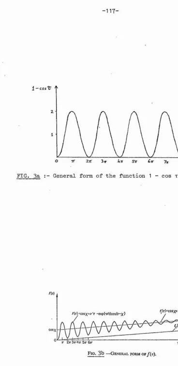
and we intend to examine the regime k^p2 >> i. The function 1 - cos x has the form sho>m in Figure (3a). Our basic assumption in the

approximation technique we now use is that the integrand in G^ contributes significantly to the integral only in regions near 1 - cos x = 0, since the integrand contains the factor exp {- k^ p2 (i - cos x)} and

k^ p2 >> 1, This assumption is supported by later computational results for the case with a collision frequency included. Thus we need only examine regions where cos x - 1 ; that is where x = 2mr + cf) with

I (j) I << 1 for n = 0» 1, 2, ...

Define the number 6^ (n = 0, 1, 2, . ...) to be the size of a

domain of significance around the point x == 2nn. By this we mean that 6 is large enough for the following inequalities to hold:-_n

exp [ s(x) ] dx >> exp [ s(x) ] dx

,2%n+6

and n exp [ s(x) ] dx >>

2n(n+l)-6^+i

exp. [s(x) ] dx

27rn-6_n 2mn+6n

for n > 1, where s(x) = iw'x - k^ p^ (1 - cos x). G^ may now be written as

"6^

Gi = exp [ s(x) ] dx

oo

+ I

n=1 _2nn-6 exp ( s(x) ] dx

-37-or, replacing t by 2irn + (j> so that

1 - cos T -X, the following approximation holds:

exp (iw'cf) - ^ } d(f)

oo

+ ^ exp {2mriw’}

n=1 exp (iw’(}> - k^ p^ } d(j>

oo

+ \ exp {2nniw*} n=1

<j> Ay Now 1 -- .cos X = ^

exp {- iw’cj) - k^pZ } d<j)

, so that the integral involving

(II.4)

exp {- k%p2 } is more convergent than the one involving

exp { - k^pZ (1 - cos X)} ; the 6^^s must also be the sizes of domains of convergence for the integrals in equation (II.4).

Therefore

<5 00

^ exp {iw'O - k^pZ ^ } dA = exp (iw’cj) - k^p^ d^

for n = 0, 1, 2, ... Consider the integral

oo

I = exp { ± iw*^ - k^ — } d(}>.

Change the variables as

follows:-r = xiil Ækp

/2 -p2

Then I = r— e _kp dp

iç-oo

= - y - z(ç) /2kp

-38-Thus from (II.4)

■i , CO

G% g - —— z( —— ) I exp (gnmiw'} v^kp v^kp n=o

CD

~ 2 ( — r— ) I exp (Snwiw'}

/2kP /2kp n=1

z ( ) (kp)'

v^kp ( 1-exp [ 2îriw*l ) Æ k

(kp)'

( 1-exp [ 2Triw'] ) -(kp)“1

If (l ~ exp [ 2iriw' ] ) is of order unity, then the contribution that Gj^ makes to a dispersion relation such as (ll.l) is quite small because of the factor (k p) ^. However, if ( 1 - exp [ 2niw' ] ) is of order

(kp) ^ , then the contribution is much more significant. This condition results in the following

cos 2niw* - 1

=> w ~ nfi for n = 0, ± 1, ± 2, ....

Bernstein showed that dispersion relations involving G^ have solutions with real w and k for w = nfi (n f O). These are known as the Bernstein modes, and they are undamped for propagation perpendicular to Bg.

Let us examine the regime k^^pZ >> -j k„^p^ > 1. We have œ

G = exp {iw'x - k^2p2 (i _ QQs T) - ikn^p^x^} dx

Making the change of variable x = 2mr + <j) as before and using the same approximations gives

00

00

exp I iw*(J) - ik^p^(f)^} d(j) ■** I exp {2nniw* - gk„^p^(2Trn)^} n=1

00

exp {<j)(iw' - k„^p^. 2mr) - gk^p^tj)^}

00

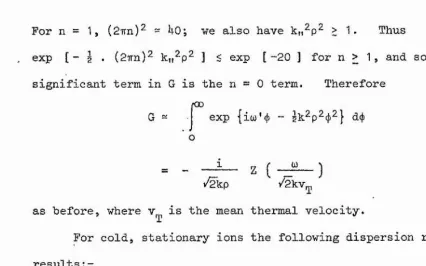
39-For n = 1, (2ïïn)^ - 40; we also have k|,^p^ > 1. Thus

exp [“ i . (2wn)2 k„^p^ ] < exp [-20 ] for n > 1, and so the only

significant term in G is the n = 0 term. Therefore

exp {iw'4> - ik^p^(j>^} d(f> roo

G “

z ( - 7 ^ )

v^kp /2kVgi

as before, where v^ is the mean thermal velocity.

For cold, stationary ions the following dispersion relation results

k.^ k 2

1 + Z' I/- ( y f - ) = 0.

k? _{2k2 T}

This is the dispersion relation for ion acoustic waves in an unmagnetized plasma with cold stationary ions. Figure (4) shows the angular regions relative to the magnetic field in which the different types of waves are important. For k,i = 0, there are undamped Bernstein waves at w = nfi for n ^ 0, and the damped n = 0 wave is in fact the ion acoustic wave. For k„2p^ << 1, the Bernstein waves are damped, but still of the

*~4o~ Chapter 3

To investigate the effect on the Bernstein modes of introducing a small amount of collisions into the plasma, we make use of theory- developed by Dougherty [ 7 ] • We provide here an outline of his procedure.

Dougherty begins with a Boltzmann equation as

follows:-I

where Einstein sums of Cartesian tensors are used, and a^ is the macroscopic acceleration vector,

collision term given by

is a Fokker-Planck

(II.5)

where

and

3v.

A. = - v(v. - u.)_{1 1 1}

V is an inverse time, independent of velocity

u^ and T are the local drift velocity

and temperature respectively, given by

nUi V. f dv_{1 —}

3 ntcT = m(v - u)2 f dv

where n is the local number density of particles, defined by n = Equation (II.5) is linearized, and written in the form

Dfi = h

where D is a linear differential operator, and f^ is given by f = fg + f1, fg being an equilibrium distribution function. Thus

h

““1

vîiere D is an inverse differential operator. Dougherty defines a set of quantities

1 . D dv

where at most two suffixes are needed before or after H. Each suffix (if any) labels the component of v to be inserted in the appropriate place in the integral.

The theory gives for f^

vTi

d“ (v2fj - 3D * f„ ] (II.6)

^1=

and the following expressions for the perturbation quantities n^, u, and T^ (ng and Tq are equilibrium values of n and T and a^ is now the

perturbed macroscopic acceleration vector )

vT

0 m

“o"i = ^ i-jj.H. 3,H)

n^ + no T1 = m 3cT,

Tr + vUj'iiHj + ^ ii«jj - 3iiH) }

We write k_m Tq as V 2 where v is the mean thermal velocity of the _{T T} particle species considered. Our procedure now differs from that of Dougherty in that we derive an expression for the charge density p(r,t), while Dougherty solves for the perturbation velocity u.

Solving equations (II.T) for u^ gives

where

M. . =

T

M. . 1.1

t no - M

3^ [ 3 ^ 2 jjH. - H. ] [ - ^ 2 -H.j - 3.H ]

n„ + !'(— &' t .^H + Hjj ] - 3H - zZT'i₃

—U2—

Substitution of u. back in (II.T) gives₁

v^ _L2 n + np - vMjj ] [ — 2 ,..H, " H, ]3vgn^ 11 j j j

Tl

Note that n^ is implicit in u^ and — , even though it is not

explicitly-involved in the expression for

To derive a dispersion relation, f^ itself is not required; the perturbed charge density p(r,t) is sufficient, and this is given as follows, using équation

(II.6):-p(r,t) = q fl(r,v,t) ^

1 vM. .

L- M 4. __ JA _{a_ D ^ (v^fg) dv}

, 1

In general a. = _{1 m - c - -} E + — v ^ B ] .₁

where E and B are the perturbed electric and magnetic fields respectively To investigate Bernstein modes, we follow Chapter 1 of this Section by making the electrostatic approximation and taking Fourier-Laplace

components, which is again equivalent to assuming a harmonic dependence of the form exp [. i(k . r ~ wt)].

The expression for a^ becomes

a. = -^ E._{1 m i}

D ^ (v^fn) dv - 3 D ^ fg dv )] (II.8)

m 3r^

where c() is an electrostatic potential independent of y. Thus

-43-taking a harmonic dependence for <}) as in Chapter 1. Therefore

! a. D (v.fg) ^ D (v.fg) -1 ÙV

m ki *

Also

and D -1 (fn ) dv = H

Ti

Substitution of these values and the expression for into (IX.8) ■‘•0

gives in terms of k and w

p(k^w) =

^

mvL

vM. . ^ ’’ ng-vM

JJ

vM. .

______ 2___JA

"o + ''(& _{'' ip} + H ] - 3H - _{J J} A_{3v^ ii"jj}t :,H.. )

mvT

vM. .

1 + --- „ . '(3^ ^ ii“j - '^dd - 3h)

n^-vM..

0 JJ _{no - v(3H +3^ ^ . .H.. - 1; [ . ,H + H. .) )_}

We now convert all Cartesian tensors to the polarized co-ordinate tensor form developed in Section I. In terms of these tensors, M.. becomes_ij

.

M

'T

3vg^ e"p

„ 0 - 3v [ H - 3^ (^H H- H^) H- ^

-44-The charge densicy is

p(k,w) = - Â U mv.T

vM

1 + ₊

Define A,

c»X-Kx)(

V

-T T

«X )

kX.

m

no-v(3H + ;%6 - Ç2 + Hg 1)

Then MP _v;T

and

p(k,w)

{ -3 [ ] A , }

-iaH vM,

1 +

no~ vMg - 3H)A, k

(II.10)

(

.

)

These expressions involve a k with general direction. We would like to investigate the effect of collisions on Bernstein modes in the region where they are most important, namely with k„ = 0 so that they are

undamped in the collisionless case. Thus in order to find p(k,(t)), we must evaluate the following set of H-functions with k„ = 0

:-H, ^ H, H*. X ,

Dougherty shows that the general H-function as follows

:-H can he evaluated

X... g

30. _{i 3p; • . . I ]o ~ p — 0}1 3 (1 1.12)

where

I = n. oo

-45-$(t)

- ~

i

\ I v2+fi2 J

1 f 1 X . 1 X . , X ( 1 - e-[^ - ' h

+ k^p, _{V + ifiX} X _X - ( V . i«X)t }_^

X = 2 tan ^ ^ ) and 0 < x < m

Note that Greek indices are used as algebraic quantities at some points in the expression for Y(t); see Appendix (ih).

For k„ = 0

#(t) = “2 • . [ cos X + vt - e cos (Ot -

x)

l4)

Since a _{and p are eventually set equal to zero, Y(t) disappears from the} final result of any integration.

The simplest H-function is H itself, given by

fOO

H = %0 exp {- $(t) + itüt) dt

and in general

00 X. . .

' *HP F^ (t) exp {- $(t) + iwt } dt

where ^ J _{••• ^ ^ ^ ^}

We now proceed to derive one of the required F’s and to list the others, in order to prevent tedious repetition. The necessary F's are the

following:-Fx' I h ' _{M ’}

where all the functions are to be evaluated with k„ = 0, that is with

0

-46-Consider the case of Fy

F 9 9

'x

= [

a = Q = 0

9Y 9Y

9a 9p^ 9a. 9p^ ]_{a = p = 0}

Now

11 3p'

( 1 - v+iww] t ) [v+iOw]t

y T I y y v + iJîy

Therefore

Similarly

11

L 3p'

1 - e [ v+ifïii] t

a = p = 0

11

]

V + inx

0 = p = 0

9^Y 90 9p'

= V 2 gA g-[v+iOy] t T p

0 ” p ~ 0

Therefore

‘F = T 2 -6^

_y

_{T p}

V + i^X V + ifîp

and

6_{F. = v„2 [g-(v+iO)t + 2-vt + g-(v - iO)t ]}

T

v / [kIk (1 - ^ (1 - ^

(p+i^)2 ^ (v-iJï)^

Now k^k = k ^ k_j = ik^ where k^ = k_t.^