Robustness Analysis of a Gradient Based Repetitive Control Algorithm

Robustness Analysis of a Gradient-based Repetitive Algorithm for

Discrete-Time Systems

Jari Hätönen, Chris Freeman, David H. Owens, Paul Lewin, Eric Rogers

Abstract— This paper investigates the possibility of using a truncated finite impulse response (FIR) model approximation to implement a well-known gradient type repetitive control algorithm. As a new result it is in fact shown that the algorithm iteratively solves a Model Predictive Control related cost function. Furthermore, it is shown how accurate the FIR approximation of the original system has to be in order for the algorithm to converge to zero tracking error. Under certain assumptions on the plant model it is shown that the algorithm results in monotonic convergence in the l∞-norm. The algorithm is applied in real-time to a non-minimum mass-damper-spring system, and experimental results are compared to the theoretical results.

I. INTRODUCTION

Many signals in engineering are periodic, or at least they can be accurately approximated by a periodic signal over a large time interval. This is true, for example, of most signals associated with engines, electrical motors and generators, converters, or machines performing a task over and over again. Hence it is an important control problem to try to track a periodic signal with the output of the plant or try to reject a periodic disturbance acting on a control system. In order to solve this problem, a relatively new research area called Repetitive Control has emerged in the control community. This study concentrates on a well-known gradient based Repetitive Control algorithm. As a new result it is shown that the algorithm iteratively solves an MPC related optimisation control using a sliding window. However, this algorithm can only be implemented causally (without prediction) if the original plant has a finite impulse response (FIR). In this nominal case the algorithm will converge to zero tracking error exponentially. If the original plant does not have a finite impulse response, the causal implementation of the algorithm requires a truncation of the response. This, however, can lead to instability, as [1] demonstrates. Therefore, as a new result, this paper estab-lishes a sufficient condition for the the FIR approximation to be accurate enough for convergence. The algorithm is also applied in real-time to a non-minimum phase spring-mass-damper system, and the experimental results give near perfect match with the theoretical findings.

Jari Hätönen and D.H. Owens are with Department of Automatic Control and Systems Engineering, University of Sheffield, Mappin Street, Sheffield S1 3JD, United King-dom,[email protected]

C. Freeman, P. Lewin and E. Rogers are with School of Electronics and Computer Science, University of Southampton, University Road, Southampton SO17 1BJ, United Kingdom

II. PROBLEM DEFINITION AND MOTIVATION As a starting point in discrete-time Repetitive Control (RC) it is assumed that a mathematical model

x(k+ 1) = Φx(k) + Γu(k)

y(k) =Cx(k) (1)

of the plant in question exists with x(0) = x₀, k ∈

[0,1,2, . . . , ∞). Furthermore, Φ, Γ, and C are finite-dimensional matrices of appropriate dimensions. For no-tational simplicity, it is assumed from now on that relative degree of the plant (1) is unity.

The design problem is to make the system (1) track a reference signalr(k), and it is known thatr(k) =r(k+N) for a given N (in other words the actual shape of r(t) is not necessarily known). In other words, the objective is to find a feedback controller that makes the system (1) to track the reference signal as accurately as possible (i.e. limk→∞e(k) = 0, e(k) := r(k)−y(k)), under the assumption that the reference signalr(k)isN-periodic. As was shown by [4], a necessary condition for asymptotic convergence is that a controller

[Su](t) = [Re](t) (2)

whereS andRare suitable operators, must have an internal model or the reference signal inside the operatorS. Because r(k) is N-periodic, its internal model is 1−σN, where

[σNv](k) =v(k−N)forv :Z→R. In the discrete-time case this requirement results in the algorithm structure

u(k) =u(k−N) + [Ke](k) (3) and if it is assumed that K is a causal LTI filter, the algorithm can be written equivalently using theq−1operator formalism as (see Section III for notation)

u(k) =q−Nu(k) +K(q)e(k) (4)

In this case the design problem is to select K(q) which results in accurate tracking but is not prone to uncertainties in the plant model. One particular way of achieving this is the algorithm (see Section III for notation)

u(k) =q−Nu(k) +βG(q−1)e(k) (5)

discussed in [1] and references therein. As is shown in Section III, this algorithm is causal, if the impulse response of the plant modelG(q)goes to zero in N steps. Section III shows that in this case the algorithm converges exponen-tially to zero, and in some special cases the convergence is monotonic in thel_∞-norm.

43rd IEEE Conference on Decision and Control December 14-17, 2004

Atlantis, Paradise Island, Bahamas

However, in practice it is quite rare the the plant model would have a finite impulse response (FIR), and the al-gorithm (5) becomes non-causal. An intuitive way of rec-tifying this problem is to truncate the plant model, or more precisely, to set the impulse of the plant model G(q) to zero after N steps, which results in causal algorithm (see also Section III). Thus this paper establishes exact conditions on how accurate the FIR approximation ofG(q) has to be in order to guarantee that the algorithm converges exponentially.

III. CONVERGENCE ANALYSIS

A. Nominal convergence

In order to introduce the necessary mathematical notation for this section, consider an arbitrary sequencef(k)∈RN. The Z-transformf(z)off(k)is defined to be

f(z) =

∞

i=0

x(i)z−i (6)

where it is assumed that f(z) converges absolutely in a region |z|> R. Dually, f(k)can be recovered from f(z) using the equation

f(k) = 1

2πi

Ωf(z)z

kdz

z (7)

where Ω is a closed contour in the region of convergence off(z). Finally, if

f(z) =f₀+f₁z−1+f₂z−2+. . . (8)

then

f(z−1) :=f₀+f₁z+f₂z2+. . . (9)

Consider now the standard left-shift operatorq−1 where

(g−1v)(k) = v(k−1) for an arbitrary v(k) ∈RZ. Using the q−1 operator, the plant equation (1) can be written as

y(k) =G(q)u(k) =C(qI−Φ)−1Γu(k) (10) where it is assumed that G(q) is controllable, observable and stable. As a more restrictive assumption, suppose that the plant has a finite impulse-response (FIR), and the length of the impulse-response is less than the length of the period N. In other words, CΦiΓ = 0 fori≥M,M < N. In the following analysis this assumption is named as the ‘FIR assumption’.

Note that the adjoint algorithm (38) can be written using the q−1-operator as

u(k) =q−Nu(k) +βG(q−1)q−Ne(k) (11)

It is important to realise that even the algorithm contains a ‘non-causal element’ G(q−1), the algorithm (11) is causal, because it can easily be seen from (11) thatu(k) =f(e(s)) fork−N≤s≤k.

The multiplication of (11) from the left with the plant model (10) together with some algebraic manipulations

(note that q−N_{r(k) = r(k)) results in the error evolution} equation

e(k) =q−N1−βG(q)G(q−1)e(k) (12) This equation can be used to establish the the convergence of the algorithm under the FIR assumption onG(q):

Proposition 1: Assume that the condition

sup

ω∈[0,2π]|1−β|G(e

jω_)|2_{|<1 (13)}

is met. In this case the tracking error e(k) satisfies that

|e(k)| ≤M αk_{for someM, α∈R,M >0, α >0,|α|<1,} and in particular,limk→∞e(k) = 0.

Remark 1: This condition can always be met, if β <

1/sup_ω∈[0,2π]|G(ejω_)|2_.

Proof. Note that by restricting time index k to lie in

[0,1,2, . . . ,∞), the error evolution equation can equiva-lently represented as an autonomous system

1−q−N(1−βG(q)G(q−1))e(k) = 0 (14)

with initial conditions e(0) = e₀, . . . , e(N −1) = en−1,

where the initial conditions are dependent on the ‘ini-tial guess’ u(0), . . . , u(N −1). According to the Nyquist stability test (see [2]), the poles of the system (14) are inside the unit circle (which guarantees that|e(k)| ≤M αk for some M, α ∈ R, M > 0, α > 0,|α| < 1), if the locus of z−N_{(1−βG(z)G(z}−1_))|

z=ejω encircles the critical point (−1,0) K times, where K is the number unstable poles ofz−N_{(1−βG(z)G(z}−1_{)). Due to the FIR}

property ofG(z), z−N_{(1−βG(z)G(z}−1_{)) does not have}

any poles outside the unit circle, and therefore, for stability z−N_{(1−βG(z)G(z}−1_))|

z=ejω is not allowed to encircle (−1,0)-point. A sufficient condition for this is

sup

ω∈[0,2π]

|(1−β|G(ejω)|2)|<1 (15)

which concludes the proof.

In summary, if the algorithm satisfies the FIR assumption, the algorithm will drive the tracking error to zero in the limit. The next subsection demonstrates that the adjoint algorithm converges monotonically to zero, if the finite impulse response of g(k) of G(q) is non-negative on the positive time-axis and goes to zero insideN time steps.

B. A note on monotonic convergence

Consider again the error evolution equation

1−q−N(1−βG(q)G(q−1))e(k) = 0 (16)

Assume without loss of generality that the impulse response of G(q) has a length of N. In this case it is easy to see that the polynomialq−N_{(1−βG(q)G(q}−1_{))has a degree}

N+N −1 (i.e. it is always odd) and therefore q−N₍₁₋ βG(q)G(q−1))can be written as

q−N(1−βG(q)G(q−1)) =

α₁q−1+α₂q−2· · ·+α₂N−1q−(2N−1)

This allows one to construct the following state-space representation for (16)

e(k+ 1) =Ae(k) (18)

where the ‘state’ e(k) is defined as e(k) := [e(k) e(k−

1) . . . e(k−(2N−1))]T _andA∈R2N−1_×R2N−1 _{is of} the form

A=

⎡ ⎢ ⎢ ⎢ ⎣

0 I 0 . . . 0

0 0 I . . . 0

..

. ... ... . .. ... α₂N−1 α2N−1 α2N−2 . . . α1

⎤ ⎥ ⎥ ⎥

⎦ (19)

Iterating (18) 2N−1 times results in

e(k+ 1) =A2N−1_{e(k−(2N−1)) (20)} which is a mapping between two consecutive cycles of length 2N. For monotonic convergence it is required that the mappingA2N−1_{has a norm less than unity in a suitable}

norm. Here the focus is on thel_∞ norm ofA2N−1_:

Proposition 2: Assume that 2_i=1N−1|αi| <1. Then the

absolute sum of each row ofA2N−1_{is less than unity, which} implies thatA2N−1

∞<1

Proof. Omitted due to space limitations.

Note that this condition can be checked numerically before applying the algorithm to the real system. The next step is to construct a connection between the condition

₂N−1

i=1 |αi|<1andsupω∈[0,2π]|1−β|G(ejω)|2|<1., i.e.

when the latter inequality implies that the first inequality holds:

Proposition 3: Assume that impulse response g(t) of

G(q)is positive, i.e.g(t)≥0fort∈[0, N]andβ satisfies

1

N

i=1g(i)2

≤β < 1

supω∈[0,2π]|G(ejω)|2

(21)

In this case supω∈[0,2π]|1−β|G(ejω)|2|< 1 implies that 2N−1

i=1 |αi|<1.

Proof. Note that sup_ω∈[0,2π]|1−β|G(ejω_)|2_{| <1 implies} that|1−β|G(1)|2|<1 and that

|1−β|G(1)|2|

=|1−β(N_i=1g(i)2−2N_k=1−1_m−n=kg(m)g(n))|

=βN_i=1g(i)2−1 + 2βN_k=1−1_m−n=kg(m)g(n))

:= Ω

(22) where 0 < m ≤ M and 0 < n < N. Note that last equality in (22) is due to the assumption that g(i)≥0 for i = 1,2, . . . N and that 1

N

i=1g(i)2 ≤ β. Furthermore, by

expandingq−N_{(1−βG(q)G(q}−1_{))as a finite power-series}

it is easily seen that

2N−1

i=1

|αi|= Ω≤λ <1 (23)

which concludes the proof.

In summary, if the impulse response is finite and positive (positivity is quite common in practical applications), and β is tuned properly, the algorithm results in monotonic convergence in the l_∞ norm for the vector e(t) defined above. Note that this result should be taken as an existence result, because in practice most of the systems do not have a finite impulse response. However, if the impulse response is positive and decays quickly to zero, it can be argued that the algorithm should result in near monotonic convergence. The experimental results in Section V support this conjecture.

C. Robust convergence

Consider not the case when a nominal plant model Go(q) is is used to approximate the true plant model G(q)(which possibly has an infinite impulse-response, IIR), where Go(q) satisfies the FIR assumption defined in the previous subsection. In this case the plant model can be written as

y(k) =G(q)u(k) =Go(q)U(q)u(k) (24)

whereU(q)is a multiplicative uncertainty that reflects the uncertainties caused by modelling errors and truncation. Again, it is assumed that each of these transfer functions are controllable, observable and stable. In this case the control law (11) with nominal model Go(q) results in the error evolution equation

e(k) =q−N_1−βG(q)G o(q−1)

e(k)

=q−N_1−βU(q)G

o(q)Go(q−1)

e(k) (25)

The following result shows a sufficient condition for con-vergence in the presence of multiplicative uncertainty:

Proposition 4: Assume that the condition

sup

ω∈[0,2π]|1−βU(e

jω_)|G(ejω_)|2_{|<1 (26)}

is met. In this case the the tracking errore(k)satisfies that

|e(k)| ≤M αk_{for someM, α∈R,M >0,α >0,|α|<1.} Proof. The proof is a trivial modification of the proof for Proposition 1. This is due to the fact that the stability assumption on U(q) guarantees no right-half poles are introduced toq−N_{(1−βU(q)G(q)G(q}−1_)).

The problem, however, is that this proposition does not reveal any information of U(q), i.e. which are the properties of U(q) that guarantee that the convergence condition in Proposition 2 is met. The next proposition shows that the phase ofU(q)is the property that can cause either convergence or divergence:

Proposition 5: Assume that U(ejω_{) satisfies that}

Proof. Note that

|1−βU(ejω_)|G(ejω_)|2_|2₌

(1−βU(ejω_)|G(ejω_)|2₎∗_(1−βU(ejω_)|G(ejω_)|2₎ = 1−βRe{U(ejω_)}|G(ejω_)|2_+β2_|U(ejω_)|2_|G(ejω_)|4

(27) where z∗ is the complex conjugate of a complex number z ∈ C. This shows immediately that if Re{U(ejω)} > 0 forω∈[0,2π],β can be be to chosen to be small enough in order to satisfy the convergence condition in Proposition

2.

Note that the condition Re{U(ejω_{)} > 0 for ω ∈ [0,2π]} is equivalent to the condition that the Nyquist-diagram of U(z) lies strictly in right-half plane. This is, on the other hand, equivalent to the phase of U(q) being inside

±90 degrees. In summary, if the phase of the nominal model Go(q) lies inside ±90 degrees ‘tube’ around the phase of the true plant G(q), there β can always made sufficiently small so that the algorithm will converge to zero tracking error. Note, however, that β ≈ 0 implies that u(k) ≈ u(k−T), which is an indication of a slow convergence rate.

IV. ACONNECTION TOMODELPREDICTIVECONTROL

In this section it will be shown that the truncated version algorithm (5) is in fact an iterative solution to a Model Predictive Control (MPC) problem. In order to achieve this, define the control vector

u(k) := [u(k)u(k+ 1) . . . u(k+N−1)]T ∈RN (28) and the corresponding tracking error vector

e(k) := [e(k+ 1) e(k+ 2) . . . e(k+N)]T ∈RN (29) where e(k) := r(k)−y(k). Consider now the following cost function

J(u(k), . . . , u(k+N−1)) :=_ik₌+_tN₊₁|e(i)|2 (30) which can be written in a more compact form as

J(u(k)) :=e(k)2₂ (31) The decision variable for the cost function is the control vector u(t)and the constraint equation is the plant model

e(k) =r(k)−y(k) =r(k)− k

i=0

h(k−i)u(i)+xo(k) (32)

where xo(t) describes the effect of non-zero initial con-ditions. Solve now this optimisation problem using the gradient method, which results in

u(k) =u(k−N)−βJ(u(k−N)) (33) Note that the plant model (32) can be written equivalently as

e(k) =r(k)−y(k) =r(k)−(Geu(k) +X0(k)) (34)

where

Ge=

⎡ ⎢ ⎢ ⎢ ⎢ ⎢ ⎣

CΓ 0 0 . . . 0

CΦΓ CΓ 0 . . . 0

CΦ2Γ CΦΓ CΓ . . . 0

..

. ... ... . .. ... CΦN−1_{Γ CΦ}N−2_{Γ CΦ}N−3_{Γ . . . CΓ}

⎤ ⎥ ⎥ ⎥ ⎥ ⎥ ⎦

(35) and X₀(k) is the initial condition response. Using this description it is easy to see that

−βJ(u(k−N)) =βGT_ee(k−N) (36) and the overall algorithm becomes

u(k) =u(k−N) +βGT_ee(k−N) (37) Furthermore, parallel to Model Predictive Control, it is proposed that a receding horizon principle should be used: in this approach only the first element u(k) of u(k) is applied to the plant, and atk+ 1the optimisation problem is solved again foru(k+1). This receding horizon principle results in the following algorithm

u(k) =u(k−N) +β N

i=1

g(N+ 1−i)e(k−i) (38)

whereg(i) =CΦi−1_{Γ, and by inspection it can bee seen}

that this algorithm is equivalent to (5). Note that in gradient based methodsβ is also optimised with respect to the cost function, and it becomes time-varying. In the RC case, however, it is not yet clear how this should be done.

V. EXPERIMENTAL WORK

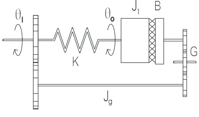
The experimental test-bed has previously been used to evaluate a number of RC schemes and consists of a rotary mechanical system of inertias, dampers, torsional springs, a timing belt, pulleys and gears. The non-minimum phase

2

2

J

B

K

G

J

o

i 1

g

Fig. 1. Non-minimum phase section

fit a linear model to a great number of frequency response test results. The resulting nominal continuous time plant transfer function has thus been established as

Go/l(s) =e−0.06s

1.202(4−s)

s(s+ 9)(s2+ 12s+ 56.25) (39)

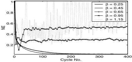
A PID loop around the plant is used since this has been found to produce superior results. This also allows the adjoint algorithm to be used with no pole-placement since the nominal closed-loop system, termed Go(s), therefore has a FIR. The PID gains are Kp = 137, Ki = 5 and Kd = 3. The impulse response of the discretized plant Go(z)is shown in Figure 2. In the experiments, the sampling frequency is set at 250 Hz (Ts = 0.004), whilst the only demand used is a repeating sequence of period 3 seconds (shown as one of the signals in Figure 7). The total number of cycles has been limited to 400.

0 1 2 3 4 5 6

−4 −2 0 2 4 6 8 10 12x 10

−3

Time (s)

Magnitude

G(jw)

Φ(jw)

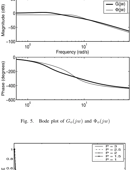
Fig. 2. Impulse responses ofG_o(jw)andΦ_o(jw)

Figure 3 shows cycle error results when the adjoint algorithm (38) is applied to the actual plant G(z). The normalised error (NE) is simply the total error produced in a period multiplied by a scalar chosen so that a constant zero plant output produces a NE of unity. The results when using increasing values of β are shown and the lack of convergence can be observed forβ≥0.65whilst instability is obvious in the case ofβ≥1.15. It follows from (13) that a sufficient condition for convergence is that, forω∈[0,2π]

−1<1−β|Go(ejωTs)|2<1 (40) and since|Go(ejwTs)| ≥0

0< β < 2

supω∈[0,2π]|Go(ejωTs)|2

(41)

The Bode plot of Go(ejωTs) is shown in Figure 5. Since the maximum value of|Go(ejωTs)|is 1.326 (2.451 dB), in this case 0 < β < 1.137 guarantees convergence for the nominal plant model. Instability, however, is seen to occur for smaller values of β when using the actual plant.

Figure 4 shows the effect of truncation on the adjoint algorithm, using G(z)andβ = 0.5. The impulse response ofGo(z)has been truncated toP seconds in the implemen-tation of the adjoint algorithm. Since the same demand is used in each case, there is no actual need for the truncation, but it is important to compare the effects of truncation under the same conditions. It has been noticed [5] that

0 100 200 300 400

0.2 0.4 0.6 0.8 1

NE

Cycle No.

β = 0.25

β = 0.45

β = 0.65

β = 0.95

β = 1.15

Fig. 3. Cycle error results using the adjoint algorithm withG(z)and variousβ

the criteria of (40) is close to being a necessary condition for convergence, as well as a sufficient one. Therefore the various results of Figure 4 which converge sucessfully are likely to converge for demands of period _P1 which have the same frequency content as the original.

0 100 200 300 400

0.2 0.4 0.6 0.8 1

NE

Cycle No.

P = 3 P = 2.5 P = 2 P = 1.5 P = 1

Fig. 4. Cycle error results using the adjoint algorithm withG(z)and variousP

In order to reduce the effect of truncation, the impulse response ofGo(z)will be shortened by using State Variable Feedback (SVF) in order to reduce the magnitude of its phase at low frequencies. Consider the plant model in (1) and the following state-feedback control law

It can be seen that the impulse response ofΦo(z)has been made nearly twice as short as that of Go(z).

100 101

−100 −50 0 50

Magnitude (dB)

Frequency (rad/s)

G(jw) Φ(jw)

100 101

−600 −400 −200 0

Phase (degrees)

Fig. 5. Bode plot ofGo(jw)andΦo(jw)

0 100 200 300 400 0.2

0.4 0.6 0.8 1

NE

Cycle No.

P = 3 P = 2.5 P = 2 P = 1.5 P = 1

Fig. 6. Cycle error results using the adjoint algorithm withΦ(z)and variousP

The adjoint algorithm has been implemented on the pole-placed system instead of the original. Figure 6 shows the effect of truncation on the cycle error results, usingβ = 0.5. The same comments as were made for Figure 4 regarding its interpretation are valid here. Truncation appears not to affect the performance of the pole-placed system for the 400 trials used. This suggests that SVF can be used sucessfully as a way of avoiding the problem of truncation when using the adjoint algorithm. This method can also be used to manipulate the system gain in order to improve convergence, although the robustness of the approach is not yet clear.

Figure 7 highlights the initial convergence of the plant output to the demand usingG(z)andΦ(z)and the adjoint algorithm with β = 0.5. It shows data from the 1st cycle and every 5th _{thereafter. Since the magnitude of}

Φo(ejwTs)is closer to

√

2than that ofGo(ejwTs)for many of the frequencies present in the demand, the RHS of (40) is reduced, and it is unsuprising that its convergence is superior.

0 5 10 15

−6 −4 −2 0 2 4 6

Output (rads)

Time (s) Demand

G(jw)

Φ (jw)

Fig. 7. Tracking of repeating sequence demand

VI. CONCLUSIONS

This objective of this paper has been to analyse the convergence properties of a well-known Repetitive Control algorithm. Due to the non-causal nature of the algorithm, the algorithm can be applied only to systems that have a finite-impulse response (FIR). Furthermore, the finite-impulse response has to go to zero at most inN steps, whereN is period of the reference signal. If the plant satisfies these assumptions, the tracking error converges to zero exponentially. When the impulse response of the plant is positive, as new result it has been shown that the algorithm results in monotonic convergence in thel_∞-norm.

If the plant does not satisfy the FIR assumption, the algorithm can be still applied by using a plant model where the impulse response is truncated after N time steps. As new result it has been shown that if the phase of the multiplicative uncertainty, which is caused by truncation, does not exceed±90degrees, the algorithm still converges exponentially to zero.

The algorithm has been applied to a non-minimum phase spring-mass-damper system. The experimental results show that the algorithm is capable of producing near perfect tracking after a small number of cycles, demonstrating that the algorithm should be applicable to industrial problems.

VII. ACKNOWLEDGMENTS

J. Hätönen is supported by the EPSRC contract No GR/R74239/01.

REFERENCES

[1] K. Chen and R. W. Longman,"Stability Issues Using FIR Filtering In Repetitive Control",Advances in the Astronautical Sciences, vol. 206, 2002, pp. 1321-1339.

[2] K. J. Astrom and B. Wittenmark,"Computer Controlled Systems: Theory and Design, Prentice-Hall, 1984.

[3] C. A. Desoer and M. Vidyasagar, Feedback Systems:Input-Output Properties, 1975, Academic Press Inc.