A bi-objective user equilibrium model of travel time reliability in a road network

This is a repository copy of

A bi-objective user equilibrium model of travel time reliability in

a road network

.

White Rose Research Online URL for this paper:

http://eprints.whiterose.ac.uk/79926/

Article:

Wang, JYT, Ehrgott, M and Chen, A (2014) A bi-objective user equilibrium model of travel

time reliability in a road network. Transportation Research Part B: Methodological, 66. 4 -

15. ISSN 0191-2615

https://doi.org/10.1016/j.trb.2013.10.007

[email protected]

Reuse

Unless indicated otherwise, fulltext items are protected by copyright with all rights reserved. The copyright exception in section 29 of the Copyright, Designs and Patents Act 1988 allows the making of a single copy solely for the purpose of non-commercial research or private study within the limits of fair dealing. The publisher or other rights-holder may allow further reproduction and re-use of this version - refer to the White Rose Research Online record for this item. Where records identify the publisher as the copyright holder, users can verify any specific terms of use on the publisher’s website.

Takedown

If you consider content in White Rose Research Online to be in breach of UK law, please notify us by

A Bi-objective User Equilibrium Model of Travel Time

Reliability in a Road Network

Judith Y.T. Wanga,c,∗_{, Matthias Ehrgott}b,c_{, Anthony Chen}d

a_{School of Civil Engineering & Institute for Transport Studies, University of Leeds, Woodhouse} Lane, Leeds LS2 9JT, United Kingdom

b_{Department of Management Science, Lancaster University, Bailrigg, Lancaster LA1 4YX, United} Kingdom

c_{Department of Engineering Science, The University of Auckland, Private Bag 92019, Auckland} 1142, New Zealand

d

Department of Civil and Environmental Engineering, Utah State University, Logan UT 84322-4110, USA

Abstract

Travel time, travel time reliability and monetary cost have been empirically

identi-fied as the most important criteria influencing route choice behaviour. We

concen-trate on travel time and travel time reliability and review two prominent user

equi-librium models incorporating these two factors. We discuss some shortcomings

of these models and propose alternative bi-objective user equilibrium models that

overcome the shortcomings. Finally, based on the observation that both models use

standard deviation of travel time within their measure of travel time reliability, we

propose a general travel time reliability bi-objective user equilibrium model. We

prove that this model encompasses those discussed previously and hence forms a

general framework for the study of reliability related user equilibrium. We

demon-strate and validate our concepts on a small three-link example.

Keywords: Route choice, user equilibrium, travel time reliability, bi-objective

∗_{Corresponding author. Tel.: +44 113 3433259 ; Fax: +44 113 343 3265.}

Email addresses:[email protected](Judith Y.T. Wang),

user equilibrium, late arrival penalty, travel time budget.

1. Introduction

1

It is well known from empirical studies that the three most important

fac-2

tors influencing route choice behaviour are travel time, travel time reliability and

3

monetary cost. Abdel-Aty et al. (1995) performed statistical analysis to

deter-4

mine which route attributes that lead to the choice of a route are considered

im-5

portant by road users. The three most important factors are: (1) shorter travel

6

time (ranked as the first reason by 40% of respondents); (2) travel time

reliabil-7

ity (32%); and (3) shorter distance (31%). Although the effect of monetary cost

8

was not considered explicitly in this study, the third most important factor, i.e.

dis-9

tance, is directly related to vehicle operating cost for the trip. In more recent years,

10

the values of travel time (VOT) and travel time reliability (VOR) were estimated in

11

two road pricing demonstrations in southern California, on California State Route

12

91 (SR91) and Interstate 15 (I-15) (see Lam and Small, 2001; Liu et al., 2004;

13

Brownstone and Small, 2005). All the analyses on these two datasets share some

14

common observations. The estimated values of VOT and VOR from these studies

15

are comparably high. For instance, the best fitted model in Lam and Small (2001)

16

has a VOT of $22.87 per hour, while the VOR is $15.12 per hour for men and

17

$31.91 for women. Note that the VOR for women is 39.5% higher than the VOT.

18

Another common observation is that substantial heterogeneity in travellers’

prefer-19

ence of travel time and reliability is observed but it is difficult to isolate its exact

20

origin (Brownstone and Small, 2005). More recently, evidence from Australian

21

case studies also indicates that drivers are willing to pay more to reduce the

uncer-22

tainty of travel time than they are for the same reduction in mean travel time (Li

23

et al., 2010).

In order to model route choice behaviour realistically, the effect of uncertainty

25

associated with travel time needs to be incorporated in the traffic assignment

proce-26

dure. The conventional user equilibrium models, namely, the user equilibrium (UE)

27

model based on Wardrop’s principle, and the stochastic user equilibrium (SUE)

28

model (Daganzo and Sheffi, 1977), do not consider the variability of travel time

29

explicitly in general. The UE model assumes that users are minimising their

gener-30

alised costs, which is often expressed as a linear combination of time and monetary

31

cost, while the SUE model assumes that users are minimising their perceived

gen-32

eralised cost, which has a randomly-distributed component.

33

A few reliability-based equilibrium models do, however, exist. These

equi-34

librium models were developed based on the concepts of travel time uncertainty

35

modelling in the empirical models. There are two main theoretical frameworks,

36

as categorised in Li et al. (2010), namely, the mean-variance model (Jackson and

37

Jucker, 1982) and the scheduling model (Small, 1982).

38

Other reliability-based equilibrium models include the travel time budget (TTB)

39

models (Shao et al., 2006a,b; Lam et al., 2008), percentile user equilibrium (PUE)

40

model (Nie, 2011), and mean-excess traffic equilibrium (METE) models (Zhou

41

and Chen, 2008; Chen and Zhou, 2010; Chen et al., 2011; Xu et al., 2013). The

42

TTB model is defined as the average travel time plus an extra time (or buffer time)

43

such that the probability of completing the trip within the TTB is no less than a

44

predefined reliability threshold alpha. The general TTB model is formulated as a

45

variant of the chance constrained model (Shao et al., 2006a,b; Lam et al., 2008),

46

where the TTB is treated as the objective function to be minimised while satisfying

47

the chance (or on-time arrival) constraint. In essence, the TTB and PUE models

48

are equivalent for any continuous distributions of random sources, while the TTB

49

model of Lo et al. (2006) derived from the mean-variance model under the normal

50

distribution assumption of route travel time is a special case. Note that the PUE

model does not assume any probability distribution for modelling capacity

uncer-52

tainty. It resorts to some convolution methods and solves the route percentile travel

53

time (or route travel time budget) numerically through the application of Fourier

54

transform (Ng and Waller, 2010; Wu and Nie, 2011).

55

The METE model is defined as the conditional expectation of the travel time

56

exceeding the TTB is defined as the conditional expectation of the travel time

ex-57

ceeding the TTB (Zhou and Chen, 2008; Chen and Zhou, 2010). As a route choice

58

criterion, the METE model can be regarded as a combination of the “buffer time”

59

measure that ensures the reliability of on-time arrival, and the “tardy time” measure

60

that represents the unreliability impacts of excessively late trips. It is a risk-averse

61

traffic equilibrium model that seeks to address two questions: “How much time

62

do I need to allow?” and “How bad should I expect from the worse cases?” The

63

issue of perception error is also considered in the stochastic version of METE by

64

explicitly modelling the stochastic perception error within the METE framework

65

(Chen et al., 2011; Xu et al., 2013).

66

For other traffic equilibrium models under uncertainty, interested readers may

67

refer to the disutility/utility-based model (Mirchandani and Soroush, 1987; Yin

68

and Ieda, 2001; Chen et al., 2002; Di et al., 2008), game theory-based models (Bell,

69

2000; Bell and Cassir, 2002; Szeto et al., 2006), the expected residual minimisation

70

approach Zhang et al. (2011), and the prospect theory-based model (Connors and

71

Sumalee, 2009; Xu et al., 2011).

72

Tan et al. (2013) investigate many of the above mentioned reliability based

73

equilibrium models and determine the shape of the mean-standard deviation

in-74

difference curves in these models. They obtain results on Pareto efficiency of the

75

equilibrium solutions of these models in terms of their Pareto efficiency regarding

76

expected travel time and standard deviation of travel time.

77

In this paper, we focus on looking at the two main theoretical frameworks,

i.e. the mean-variance model and the scheduling model, from a multi-objective

79

perspective. Now we look into these two models in more detail.

80

In the mean-variance model, Jackson and Jucker assume that travel time

vari-81

ability leads to loss of utility. Every traveller has a prior estimate of the mean

82

and variance of the travel time and the objective of each traveller is expressed by

83

Equation (1).

84

min{E(Tk) +λmV (Tk) :k∈Kp}, (1)

whereλm is a non-negative parameter which represents the degree to which the

85

variability of travel time is undesirable to travellerm;E(Tk)is the expected travel

86

time on pathkfor O-D pairp;V (T_k)is the variance of the travel time on pathk;

87

andKpis the set of all paths for O-D pairp. Variations of the mean-variance model,

88

such as the mean-standard deviation model, constant relative risk aversion (CRRA)

89

model, and constant absolute risk aversion (CARA) model, have also been

consid-90

ered in de Palma and Picard (2005) to model different risk aversion preferences

91

towards travel time uncertainty.

92

In the scheduling model, Small assumes that not arriving at the destination at

93

the preferred arrival time (PAT) will cause disutility, and the consequence of

ar-94

riving early and late could be different. Naturally one would expect that travellers

95

would dislike being late more than being early. The utility function can be

ex-96

pressed as in Equation (2).

97

U(td;PAT) =α1T+α2SDE+α3SDL+α4DL, (2)

where td is the decision variable, the departure time choice; PAT is a preferred

98

arrival time;T is the travel time;SDEis the scheduling delay early as defined in

99

Equation (3);SDLis the scheduling delay late as defined in Equation (4); andDL

100

is a binary variable indicating whether it is a late arrival or not (DL= 1if and only

ifSDL >0); and the estimated parameters (α₁, α₂, α₃andα₄) are assumed to be

102

negative.

103

SDE = max (0,PAT−[T+td]), (3)

SDL = max (0,[T+td]−PAT). (4)

Now let us look at how these concepts have been applied in equilibrium models.

104

Based on the concept in the mean-variance model, Lo et al. (2006) formulated

105

a multi-class equilibrium model by considering a single objective as minimising

106

travel time budget, defined as the expected travel time plus a travel time margin

107

(or buffer time), with the travel time margin being dependent on the level of risk

108

aversion of each user class, as shown in Equation (5).

109

Bk=E(Tk) +λmσTk, (5)

for allk ∈ Kp (the set of all paths from origin to destination of O-D pairp) and

110

for allp ∈ Z (the set of all O-D pairs), whereB_k is the travel time budget;T_k

111

is the random variable of travel time on routekfor O-D pairp;E(Tk) andσTk,

112

respectively, are the mean and standard deviation ofT_k.λmis a parameter

associ-113

ated with the level of risk aversion of individualm. Note that although the travel

114

time budget model shares a similar mathematical form with the mean-variance (or

115

standard deviation) model, it has a different meaning defined by the travel time

116

reliability chance constraint such that the probability that travel time exceeds the

117

budget is less than a predefined confidence level specified by the traveller to

rep-118

resent his/her risk preference. Lo et al. (2006) called this the within budget time

119

reliability (WBTR) or the punctuality reliability. This definition is also similar to

120

the alpha-reliable route defined by Chen and Ji (2005) to indicate the route with

121

the minimum travel time budget.

Based on the concept of aschedule delaycomponent in the scheduling model,

123

Watling (2006) proposed a late arrival penalised UE (LAP-UE) which assumes

124

users minimise a composite path disutility, incorporating the generalised cost plus a

125

late arrival penalty. Watling (2006) assumes that travellers make their route choice

126

decision with a longest possible travel time in mind for their journey. If this is

127

exceeded, the inconvenience incurred will be modelled by the penalty component

128

of the utility function in Equation (6).

129

U(k;τm) =θ0dk+θ1E(Tk) +θ2E[max (0, Tk−τm)], (6)

wherekis the decision variable, the path choice, with a longest acceptable travel

130

timeτmin mind. Further,θ0dk+θ1E(Tk)is the standardgeneralised travel time

131

andθ2E[max (0, Tk−τm)]is the penalty component. In particular,dkrepresents

132

the composite of attributes (such as distance) that are independent of time and flow;

133

E(Tk) is the mean travel time on routek;θ2 is the value of being one time unit

134

later than acceptable; and the estimated parameters(θ0, θ1, θ2)are assumed to be

135

negative.

136

The models in Lo et al. (2006) and Watling (2006) both incorporate the effects

137

of travel time and its uncertainty. Lo et al. (2006) use the buffer time,λmσTk in

138

Equation (5), while Watling (2006) uses the penalty function,θ2E[max (0, Tk−

139

τm)] in Equation (6). Although they use two different measures to model the

140

effect of unreliability on route choice, the models share the same assumption that

141

the effects of these two factors can be combined into a single objective with a linear

142

disutility function. Based on the results from empirical studies as discussed earlier,

143

one would expect that a route choice decision is in fact a multi-criteria decision

144

based on important factors such as expected travel time and its variability. In fact,

145

combining the two key factors into one implicitly assumes the existence of a linear

146

(dis)utility function, and therefore pre-supposes a certain preference structure. As

an effect of this, there is the possibility that somereasonable choices are never

148

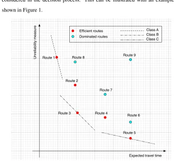
considered in the decision process. This can be illustrated with an example as

149

shown in Figure 1.

150

Class A Class B Class C

U

n

re

lia

b

ili

ty

me

a

su

re

Expected travel time Route 1

Route 2

Route 3 Route 4

Route 5 EfÞcient routes

Dominated routes

Route 9 Route 8

Route 7

Route 6

Figure 1: Trade off between expected travel time and unreliability measure

In Figure 1, the travel time reliability of nine possible routes between one

151

origin-destination pair is plotted against their corresponding expected travel time.

152

The measures of reliability can be, say the buffer times,λmσTk, in Lo et al.’s

for-153

mulation or the late arrival penalty in Watling’s. As all travellers would want to

154

minimise these two objectives, a set of efficient options among the nine

alterna-155

tives can be identified, which are represented by Routes 1 to 5 in Figure 1. Routes

156

6 to 9 will not be considered by a rational traveller, as they are dominated by at

least one other route, which has no worse expected travel time and buffer time,

158

but is better in at least one of these criteria. In the equilibrium model of Lo et al.

159

(2006), the different levels of risk aversion are modelled by different values ofλm

160

for different user classes in the objective function, Equation (5). Graphically, the

161

objective functions of different user classes can be represented by the dotted lines

162

with different slopes in Figure 1, whereλmis the slope of the line. As a result, the

163

optimal choices of Classes A, B and C will all be different: They are Routes 1, 3

164

and 5, respectively. Although Routes 2 and 4 are bothefficientroutes in this case,

165

i.e. there are no other routes with expected travel time and travel time variability

166

less than or equal to those of Routes 2 and 4 and at least one of these criteria

bet-167

ter, they will never be chosen by any travellers according to this model. This is

168

because the linear combination ofE(Tk)andσTk in the objective function will not

169

be able to completely represent a bi-objective decision process. Replacing buffer

170

time by lateness penalty E[max(0, Tk−τm)], a similar argument can be made

171

for the LAP-UE model of Watling (2006). We note that Dial (1997) suggests a

172

similar formulation to Lo et al. (2006), without explicitly specifying the reliability

173

measure. Dial’s model will, therefore, have the same issue as illustrated in this

174

example.

175

While missing out somerational alternatives is a general problem that needs

176

to be addressed, there are some other properties of this decision process that a

177

single objective formulation might not be able to address. For instance, in the time

178

budget equilibrium model (Lo et al., 2006), all the used routes at equilibrium will

179

have equal travel time budget for the users in the same class. This means that the

180

used routes even for the same user class can have different expected travel times

181

as well as different travel time margin, as long as the sums, i.e. the travel time

182

budgets, are equal and minimal.

183

This condition implicitly implies two characteristics at equilibrium. Firstly,

since the travel time budget on all used routes is equal, the departure time relative

185

to the same desired arrival time window of users in the same class will all be the

186

same. Secondly, the choice set for users in the same class consists of routes with

187

different expected travel time but the users are indifferent towards these different

188

travel times as long as the travel time budget on each route is the same and

min-189

imal. In other words, a used route with a lower expected travel time but higher

190

variability is equally attractive as another route with a higher expected travel time

191

but lower variability as long as the travel time budgets on the two routes are the

192

same. This might not be true as some users might prefer to spend less time in

traf-193

fic on average. In that case, the route with the shortest expected travel time would

194

be the most attractive. Once we introduce the mathematical formulation of the late

195

arrival penalty user equilibrium model (Watling, 2006) in Section 3, it is easy to

196

see that a similar comment applies for that model, too.

197

In this paper, we address the possibility that users’ travel time margin not only

198

varies between different user classes but also within the same class and users’

pref-199

erence is not only dependent on travel time budget but on both the expected travel

200

time and travel time budget. We propose a new modelling framework to model

201

such conditions with a travel time reliability bi-objective user equilibrium

(TTR-202

BUE) model. The idea of bi-objective user equilibrium was introduced in Wang

203

et al. (2010) in the context of tolling analysis, but can be adapted to any modelling

204

framework in which we expect users might react differently to several objectives

205

influencing their route choices. Our research also contributes to the growing

liter-206

ature that uses multi-objective methods in a variety of transportation research

con-207

texts, such as Tan and Yang (2012), who study built-operate-transfer contracts in

208

the context of optimising social welfare and private profit; Chen and Yang (2012),

209

who consider minimising the conflicting social costs of congestion and emissions

210

with toll schemes and Yang et al. (2012), who consider speed limits to obtain

cient flow patterns in terms of reducing both total travel time and total emissions.

212

In Sections 2 and 3, we will describe the travel time budget and late arrival

213

penalty user equilibrium models mathematically. We also introduce bi-objective

214

versions of these models, and prove that the equilibrium solutions of the models

215

of Lo et al. (2006) and Watling (2006) are special cases of the corresponding

bi-216

objective user equilibrium models. In Section 4, we present a new general travel

217

time reliability bi-objective user equilibrium model, which eliminates the need for

218

user-class-specific parameters and preference assumptions. We prove that all four

219

models mentioned in Sections 2 and 3 are special cases of this general model.

220

Hence, the general model serves as a modelling framework for the study of travel

221

time reliability. We demonstrate our concepts on a small example in Section 5 and

222

draw some conclusions and suggestions for further work in Section 6.

223

2. Travel Time Budget User Equilibrium

224

The travel time budget user equilibrium focuses on modelling the travel

be-225

haviour of road users in response to the day-to-day variations in travel time

in-226

duced by disruptions on a minor scale, caused by traffic incidents. We, therefore,

227

adopt the results from Lo and Tung (2003), summarised as follows. Throughout

228

the paper, the Bureau of Public Roads (1964) link performance function

229

ta(fa) =t0a

1 +β

fa Ca

n

(7)

is adopted, wheret0_ais the free-flow travel time and Ca is the capacity of linka.

230

Thus, ta(fa) is the link travel time with link flowfa andβ, n are deterministic

231

parameters.

232

Lo and Tung (2003) assume that link capacity follows a uniform distribution,

233

defined by an upper bound (the design capacity) and a lower bound (the

worst-234

degraded capacity), which is a fraction,φa, of the design capacity,¯ca, i.e.

Ca∼U(φa·c¯a,¯ca). (8)

Henceφaserves the role as a reliability parameter for travel time: As derived

236

in Lo and Tung (2003), the path travel time is normally distributed with mean and

237

standard deviation that can be written as

238

Tk ∼ N(E(Tk), σTk) (9)

E(Tk) = X

a h

δk_a·E(ta) i

(10)

σT_k = s

X

a

[δk

a·var(ta)]. (11)

Hereδk_ais the usual link-path incidence, i.e.δk_a = 1if linkabelongs to pathkand

239

0 otherwise. By applying the assumption of uniformly distributed arc capacity as

240

expressed in Equation (8), the mean and standard deviation of the route travel time

241

distribution are

242

E(T_k) =X

a

δk_a·

t0_a+βt0_af_an 1−φ 1−n a

¯

cn

a(1−φa) (1−n)

, (12)

σTk =

v u u t

X

a "

δk

a·β2(t0a)2fa2n (

1−φ1a−2n

¯

c2n

a (1−φa) (1−2n) −

1−φ1a−n

¯

cn

a(1−φa) (1−n) 2)#

.

(13)

The travel time budget model of Lo et al. (2006) is a multi-user class

equilib-243

rium model which considers both the expected travel timeE(Tk)and the variability

244

of travel time, as measured byσTk with users in classm minimising their travel

245

time budget Bk = E(Tk) +λmσTk. Mathematically, λm can be related to the

246

probabilityρmthat a trip arrives within the travel time budget,

247

After rearranging (14), we have

248

P

STk =

Tk−E(Tk) σT_k 6λm

=ρm. (15)

Note that the left hand side in Equation (15) is the standard normal variate ofTk,

249

STk ∼N(0,1).

250

As pointed out in Section 1, in any solution of the travel time budget

equilib-251

rium problem, it is possible that for a given user classm, there are several paths

252

with equal and minimal time budget. As mentioned before, users in the same class

253

would be indifferent with respect to such paths. We believe that this might not

254

be realistic and suggest a bi-objective user equilibrium model that overcomes this

255

problem.

256

Now let us consider the formulation in Lo et al. (2006) from a bi-objective

per-257

spective. The travel time budget represents how much time needs to be allowed

258

for the trip while the expected travel time represents how much time is expected to

259

be spent in traffic. One would expect that users will always want: (1) to minimise

260

the expected travel time, i.e.minE(Tk); and (2) to minimise the travel time

bud-261

get, i.e.minBk, subject to an acceptable level of risk. As explained above, risk is

262

represented by the probability of the actual travel time being longer than the travel

263

time budget.

264

Mathematically, the two objectives are:

265

minE(Tk), (16)

minBk=E(Tk) +λmσTk,

whereBkis dependent on the level of risk aversion of the individual or user class

266

m, measured byρm, which determines the value ofλmas in Equation (15), i.e.Bk

267

is the objective function of the travel time budget model.

Based on the objective functions in (16), we can formulate the travel time

bud-269

get bi-objective user equilibrium (TTB-BUE) as follows.

270

“Undertravel time budget bi-objective user equilibriumconditions

271

traffic arranges itself in such a way that no individual trip maker can

272

improve either his/her expected travel time or travel time budget or

273

both without worsening the other objective by unilaterally switching

274

routes.”

275

We will show that every solution of the travel time budget equilibrium model

276

of Lo et al. (2006) is also a solution to at least the weak TTB-BUE model. To that

277

end, we define the weak TTB-BUE model.

278

“Underweak travel time budget bi-objective user equilibrium

con-279

ditions traffic arranges itself in such a way that no individual trip maker

280

can improve both his/her expected travel time and travel time budget

281

by unilaterally switching routes.”

282

Theorem 1. LetF be a path flow solution to the travel time budget equilibrium

283

model. ThenFalso satisfies the weak TTR-BUE condition.

284

Proof. Assume thatF does not satisfy the weak TTR-BUE condition. Then, for at

285

least one user classmthere must exist two used pathskandk′between some O-D

286

pairpsuch thatE(Tk′) < E(T_k)andE(T_k′) +λ_mσ_T

k′ < E(Tk) +λmσTk. The

287

second of these inequalities contradicts the assumption that_F satisfies the travel

288

time budget equilibrium condition.

289

3. Late Arrival Penalty User Equilibrium

290

Based on the concept ofschedule delay, as introduced by Small (1982), Watling

291

developed the idea of a schedule delay equilibrium model, known as LAP-UE

(Watling, 2006) as described earlier. The assumption behind this model is that

293

users are concerned about expected travel time as well as the expected schedule

294

delay given a longest possible travel timeτm(for user classm).

295

Based on Watling (2006)’s derivation, the schedule delayE[max(0, Tk−τm)]

296

in Equation (6) can be simplified to Equation (17) whereL(x)is given in Equation

297

(18).

298

E[max (0, Tk−τm)] =σTkL

τm−E(Tk) σT_k

, (17)

L(x) = Z inf

x

(u−x)φ(u)du=φ(x) +xΦ (x)−x, (18)

where φ and Φ are the probability density function and cumulative distribution

299

function of aN(0,1)variate, respectively. In the LAP-UE model, users minimise

300

Equation (6). In this study, we are not concerned with attributes that are

indepen-301

dent of time or flow, hence we assume thatθ₀ = 0and we can normaliseθ₁ to 1.

302

This also puts the discussion of the model of Watling (2006) in the same framework

303

as that of Lo et al. (2006), where travel time independent factors are not considered.

304

The user objective becomes the disutility of pathk

305

minu_k=E(T_k) +θ₂L

τm−E(Tk) σTk

σTk. (19)

We have mentioned before that this model leads to a similar problem to that

306

of Lo et al. (2006): There might be several paths with the same minimal value

307

ofuk that have differing expected travel times (and, therefore, different late

ar-308

rival penalties). The model implicitly assumes that users are indifferent to these

309

paths. To avoid this, we can proceed in the same way as for the model of Lo et al.

310

(2006) by considering the model from a bi-objective perspective and separate the

311

two components ofukout. That is, we assume users would want: (1) to minimise

312

expected travel time; and (2) to minimise the expected schedule delay or lateness

313

penalty.

Mathematically, the two objectives are:

315

minE(Tk), (20)

minE[max (0, Tk−τm)].

With these objectives, we can define the late arrival penalty bi-objective user

316

equilibrium (LAP-BUE) as follows.

317

“Under late arrival penalty bi-objective user equilibrium

condi-318

tions traffic arranges itself in such a way that no individual trip maker

319

can improve either his/her expected travel time or late arrival penalty

320

or both without worsening the other objective by unilaterally

switch-321

ing routes.”

322

As for the time budget model, we now proceed to show that a solution to the

323

LAP-UE model is always a solution to the LAP-BUE model.

324

Theorem 2. LetFbe a path flow solution to the late arrival penalty user

equilib-325

rium model. ThenFalso satisfies the LAP-BUE condition.

326

Proof. Assume that_Fdoes not satisfy the LAP-BUE condition. Then, for at least

327

one user classm there must exist two used paths k and k′ such that E(Tk′) 6

328

E(Tk) andL _τ

m−E(Tk′)

σT k′

σT_k′ 6 L

τm−E(Tk)

σ_Tk

σTk, with at least one of these

329

inequalities strict. But this implies that

330

E(Tk′) +θ₂L

τm−E(Tk′)

σTk′

σTk′ < E(Tk) +θ2L

τm−E(Tk) σTk

σTk

contradicting the LAP-UE condition.

331

Under the LAP-BUE condition, if several paths with the same minimal value

332

ofuk exist, users would always prefer the one which has lower expected travel

time. We may also use this LAP-BUE model as a tie-breaker in the conventional

334

user equilibrium model considering only (generalised) travel time: Faced with the

335

choice between two paths with equal expected travel time, users would prefer the

336

one which has lowest schedule delay.

337

4. The General Travel Time Reliability Bi-objective User Equilibrium

338

In Sections 2 and 3, we have briefly presented the travel time budget user

equi-339

librium (Lo et al., 2006) and late arrival penalty user equilibrium (Watling, 2006)

340

models as the main network equilibrium models in the literature that consider

ex-341

pected travel time as well as standard deviation of travel time in a network

equilib-342

rium model. We have illustrated that the implicit assumption of user indifference

343

towards the two components of the function used in these models creates

ambi-344

guity, and that it may not be realistic to assume that users are indifferent towards

345

the different expected travel times that used paths in an equilibrium solution may

346

have. We have suggested bi-objective user equilibrium models to overcome these

347

problems. In this section, we propose a general travel time reliability bi-objective

348

user equilibrium model (TTR-BUE) that incorporates both the original TTB-UE

349

and LAP-UE models, as well as their bi-objective counterparts (16) and (20) and

350

other possible reliability models. From now on, we omit the assumption of normal

351

distribution of travel time, which Watling used and which Lo and Tung (2003)

ob-352

tained from the assumption of uniform distribution of capacity, and only assume

353

that travel time follows a distribution such that expected (path) travel time as well

354

as standard deviation of (path) travel time are continuous and positive functions

355

of flow. Note that Equations (12) and (13) meet this assumption. Therefore, the

356

assumptions of the travel time budget model of Lo et al. (2006) are more restrictive

357

than the assumptions for our model.

The common feature of all models discussed so far is that they consider

ex-359

pected travel time E(Tk) as well as a reliability component, with the reliability

360

component modelled as either travel time margin in Lo et al. (2006) or lateness

361

penalty in Watling (2006).

362

We observe that both Equations (5) from Lo et al. (2006) and (6) from Watling

363

(2006) with the reformulation (17) contain the standard deviation of travel time

364

σTk weighted by either a constantλmor the constantθ2multiplied by functionL,

365

which itself depends onE(Tk) andσTk. Clearly, bothλm andL are user (class)

366

dependent. Recall that λm is derived from the level of risk aversion of user m

367

(see Equations (14) and (15)), and thatL in (19) containsτm as the maximum

368

conceivable travel time of usermas a parameter.

369

We now postulate that the essential components of travel time reliability

equi-370

librium models are expected travel time E(Tk) and standard deviation of travel

371

timeσTk. We will not make any further assumptions on how to combine these two

372

factors into a single objective function such as Equations (5) and (19) do. Hence,

373

we do not assume the existence of a valueλmthat allows a weighting of travel time

374

reliability (standard deviation) relative to expected travel time nor do we assume

375

that users make their path choice based on the schedule delay model. Instead, we

376

only assume that users will always want: (1) to minimise the expected travel time,

377

i.e.minE(Tk); and (2) to maximise travel time reliability, or alternatively, to

min-378

imise the standard deviation of travel time, i.e.minσTk. Note that based on this

379

assumption, we are modelling users who are either risk neutral or risk averse, but

380

not risk prone. As a result, the value ofλmwill always be greater than zero.

381

In this way, we consider the problem from a multi-objective point of view and

we can formulate a general TTR-BUE model with the two objectives

383

minE(Tk), (21)

minσTk.

We consider this formulation general in the sense that we assume that

trav-384

ellers perceiveunreliabilitysolely based on the variability of travel time, which is

385

measurable as the standard deviation. The general TTR-BUE condition reads as

386

follows.

387

“Undertravel time reliability bi-objective user equilibrium

condi-388

tions traffic arranges itself in such a way that no individual trip maker

389

can improve either his/her expected travel time or standard deviation

390

of travel time or both without worsening the other objective by

unilat-391

erally switching routes.”

392

Based on this definition, all the used routes between a given O-D pair are

effi-393

cient. For an efficient route, there does not exist any alternative route that has lower

394

expected travel time or lower standard deviation unless the other component is

big-395

ger. This means every routedominatedby an efficient route, i.e. one which has at

396

least the same or higher expected travel time as well as at least the same or higher

397

standard deviation of travel time, as compared with the efficient route should have

398

zero flow. This assumption appears to be realistic for rational users.

399

Next we give a mathematical statement of the TTR-BUE model as an

equilib-400

rium problem. For notational simplicity, we only state it for a single user class.

401

Let us first introduce the necessary notation. LetG= (N, A)be a network, where

402

N is a finite set of|N|nodes andA ⊂ N ×N is a set of|A|arcs or links. Let

403

Z ⊂N ×N be a set of origin-destination pairs (O-D pairs) and for allp∈Z, let

404

Dpdenote the demand for travel between O-D pairp. The set of all paths between

O-D pairpis denotedKpandK:=∪pinZKpis the set of all paths. LetF∈R|K|

406

be a path flow vector that satisfies demand, i.e. P

k∈KpFk = Dp for allp ∈ Z.

407

Finally, letCk(F) := (E(Tk), σTk)

T _{be the vector containing the expected travel}

408

time and standard deviation of travel time of pathk.

409

Definition 1. Path flow vectorFis a travel time reliability bi-objective user

equi-410

librium flow ifFis feasible, i.e. F≥ 0,P

k∈KpFk = Dp for allp ∈Z, and the

411

following conditions hold.

412

1. If for anyp ∈ Z and any k, k′ ∈ Kp it holds that Ck′(F) ≤ C_k(F) and

413

Ck′(F)6=C_k(F)thenF_k= 0.

414

2. If for anyp∈Z andk∈ Kpit holds thatFk >0then there is nok′ ∈ Kp

415

withFk′ >0such thatC_k′(F)≤C_k(F)andC_k′(F)6=C_k(F).

416

Notice that the TTB-BUE and LAP-BUE solutions in Sections 2 and 3 are

417

formally defined in the same way as TTR-BUE in Definition 1, but with the cost

418

functions of Equations (16) and (20) rather than (21). We now show that under

419

our assumptions thatE(Tk)andσTkare positive and continuous functions of flow,

420

travel time reliability bi-objective user equilibrium flows exist.

421

Theorem 3. LetG= (N, A)be a network,Z⊂N×N be a set of O-D pairs and

422

for allp∈Z, letDpbe the demand of O-D pairp. Assume that both cost functions

423

C_k(i)(F), i = 1,2 are positive and continuous. Then a travel time reliability

bi-424

objective user equilibrium flow exists.

425

Proof. Because of the assumption thatE(Tk)andσTk are positive and continuous

426

functions of flow, we know that the time budget function Bk(F) := E(Tk) +

427

λσTk for positive λ is positive and continuous. Hence an equilibrium flow F

∗

428

with respect toBk exists. We show that this equilibrium flowF∗ is a TTR-BUE

429

flow. Assume to the contrary that there is an O-D pairpand two pathsk, k′ ∈Kp

with positive flow such thatC_k′(F∗) ≤ C_k(F∗) and C_k′(F) 6= C_k(F). Then

431

Bk′(F∗) < B_k(F∗) contradicting the fact that F∗ is an equilibrium flow with

432

respect toBk.

433

This model can capture all the possible equilibria based on our definition of

434

TTR-BUE without specifying how travellers might respond to the uncertainty in

435

travel time associated with each route as modelled by standard deviation of travel

436

time. We now prove that both the TTB-BUE model (and hence the TTB-UE model)

437

and the LAP-BUE model (and hence the LAP-UE model) are special cases of our

438

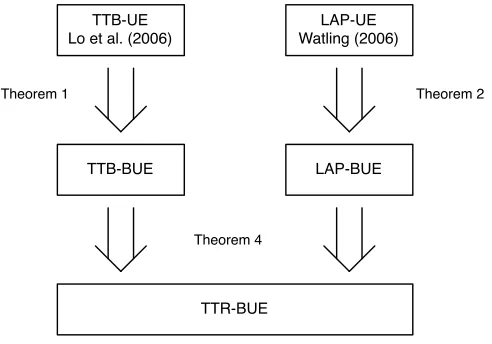
new general TTR-BUE model, see Figure 2, which summarises the results of

The-439

orems 1, 2 and 4.

440

Theorem 4. The following two statements hold.

441

1. LetFbe a path flow solution of the TTB-BUE model. ThenFalso satisfies

442

the TTR-BUE condition.

443

2. LetFbe a path flow solution of the LAP-BUE model. ThenFalso satisfies

444

the TTR-BUE model.

445

Proof. We prove both statements separately.

446

1. If_Fdoes not satisfy the TTR-BUE condition, there must exist a user classm

447

and two pathskandk′between an O-D pairpsuch thatE(Tk′)6E(T_k)and

448

σT_k′ 6σTk with at least one strict inequality. Then, becauseλmis positive

449

in the TTB-BUE model, we must haveE(Tk′) +λ_mσ_T

k′ < E(Tk) +λmσTk.

450

This combined withE(Tk′) 6E(T_k)shows thatFwould then also violate

451

the TTB-BUE condition.

452

2. Assume_Fsatisfies the LAP-BUE but not the TTR-BUE conditions. Then,

453

as in the proof of the first statement, there must exist a user class m and

454

two pathskandk′ between an O-D pairpsuch thatE(Tk′) 6 E(T_k)and

σT_k′ 6 σTk with at least one strict inequality. It is well known that L(x)is

456

a decreasing function ofx. HenceLτm−E(Tk)

σ_Tk

increases as bothE(Tk)

457

andσTk increase and therefore

458

L

τm−E(Tk′)

σT_k′

σT_k′ 6L

τm−E(Tk) σT_k

σTk,

which, with an analogous argument as in the proof of the first statement,

to-459

gether withE(Tk′)6E(T_k)and the fact that at least one of the inequalities

460

must be strict, contradicts the LAP-BUE condition.

461

462

TTB-UE Lo et al. (2006)

LAP-UE Watling (2006)

TTB-BUE LAP-BUE

TTR-BUE

Theorem 1 Theorem 2

Theorem 4

Figure 2: The relationship between single objective and bi-objective user equilibrium models for

travel time reliability.

At this stage, we need to point out that the TTR-BUE model is not in itself

463

suitable to derive a particular equilibrium solution, but only serves as a framework,

464

identifying a range of solution within which any equilibrium based on expected

465

travel time and standard deviation of travel time as the route choice criteria must

fall. The computation of this range of solutions is difficult, and the development of

467

algorithms to do this is the subject of further research.

468

5. A Three-link Example

469

In this section, we demonstrate and validate our concepts with a simple

three-470

link example as follows.

471

5.1. Network Specification

472

Our test three-link network is shown in Figure 3, where the link parameters are

473

specified in Table 1. The parameters of the travel time function, Equation (7), are

474

β = 0.15andn = 4. The total demand is assumed to be fixed at 15,000 vehicles

475

per hour. For simplicity, we consider a single user class.

476

r s

1

2

3

Figure 3: A three-link example network.

Note that in Table 1, we specify a travel time reliability parameter of φa for

477

routeaas defined in Equation (8). Theφ−value for the expressway is the lowest,

478

meaning that it is the route that could be most degradable although it is the shortest,

479

while the arterial route is assumed to be the most reliable with the highestφ−value.

480

5.2. The TTR-BUE Solution Space

481

As the demand is fixed, the solution space for this three-link network can be

482

represented two-dimensionally with the horizontal axis and the vertical axis

Table 1: Route characteristics of the three-link network.

Route Type Distance Free flow Capacity Reliability

travel time

a (km) (mins) (veh/hr) φa

1 Expressway 20 12 4000 0.5

2 Highway 50 30 5400 0.7

3 Arterial 40 40 4800 0.9

resenting the flows on Routes1 and2, respectively. In order to illustrate the set

484

of solutions of the three bi-objective user equilibrium models in this three-link

485

example, we first discretise the two-dimensional solution space and identify the

486

solutions for each of the three cases as formulated in Sections 2, 3 and 4. For each

487

feasible solution, we can evaluate the corresponding travel time and travel time

re-488

liability on each of the three routes. We can then determine whether all the three

489

data points are efficient based on the concept illustrated in Figure 1. If all three

490

routes are efficient, the solution is within the BUE region.

491

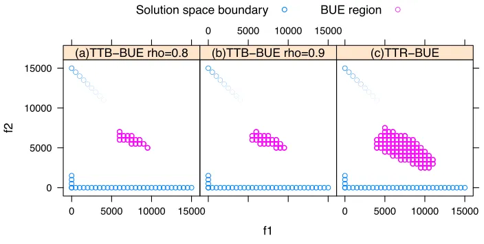
5.2.1. Travel Time Budget (TTB) Versus General (TTR) BUE

492

The solution sets of the TTB-BUE formulation for different levels of risk

aver-493

sion (withρ−values of 0.8 and 0.9) are compared with that of the general

TTR-494

BUE formulation in Figure 4. As predicted by Theorem 4, comparing Figures 4 (a)

495

& (b) with Figure 4 (c), the TTB-BUE solution sets are within the general

TTR-496

BUE region. By comparing Figures 4 (a) and (b), a higher level of risk aversion

497

leads to a bigger solution set.

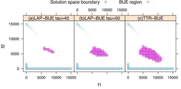
5.2.2. Late Arrival Penalty (LAP) Versus General (TTR) BUE

499

The solution sets of the LAP-BUE formulation for different levels of risk

aver-500

sion (withτ−values of 40 and 50 minutes) are compared with that of the general

501

TTR-BUE formulation in Figure 5. As stated by Theorem 4, comparing Figures

502

5 (a) & (b) with Figure 5 (c), the LAP-BUE solution sets are within the general

503

TTR-BUE region. By comparing Figures 5 (a) and (b), a higher time allowance

504

leads to a bigger solution set.

505 f1 f2 0 5000 10000 15000

0 5000 10000 15000 ● ● ● ● ● ● ● ● ● ● ● ● ● ● ● ● ● ● ● ● ● ● ● ● ● ● ● ● ● ● ● ● ● ● ● ● ● ● ● ● ● ● ● ● ● ● ● ● ● ● ● ● ● ● ● ● ● ● ● ● ● ● ●●●●●●●●●●●●●●●●●●●●●●●●●●●●●●● ● ● ● ● ● ● ● ● ● ● ● ● ● ● ● ● ● ● ● ● ● ● ● ● ● ● ● ● ● ● ● ● ● ● ● ● ● ● ● ● ● ● ● ● ● ● ● ●

(a)TTB−BUE rho=0.8

0 5000 10000 15000

● ● ● ● ● ● ● ● ● ● ● ● ● ● ● ● ● ● ● ● ● ● ● ● ● ● ● ● ● ● ● ● ● ● ● ● ● ● ● ● ● ● ● ● ● ● ● ● ● ● ● ● ● ● ● ● ● ● ● ● ● ● ●●●●●●●●●●●●●●●●●●●●●●●●●●●●●●● ● ● ● ● ● ● ● ● ● ● ● ● ● ● ● ● ● ● ● ● ● ● ● ● ● ● ● ● ● ● ● ● ● ● ● ● ● ● ● ● ● ● ● ● ● ● ● ● ● ● ● ● ● ● ● ● ● ● ● ● ● ● ● ● ● ●

(b)TTB−BUE rho=0.9

0 5000 10000 15000 ● ● ● ● ● ● ● ● ● ● ● ● ● ● ● ● ● ● ● ● ● ● ● ● ● ● ● ● ● ● ● ● ● ● ● ● ● ● ● ● ● ● ● ● ● ● ● ● ● ● ● ● ● ● ● ● ● ● ● ● ● ● ●●●●●●●●●●●●●●●●●●●●●●●●●●●●●●● ● ● ● ● ● ● ● ● ● ● ● ● ● ● ● ● ● ● ● ● ● ● ● ● ● ● ● ● ● ● ● ● ● ● ● ● ● ● ● ● ● ● ● ● ● ● ● ● ● ● ● ● ● ● ● ● ● ● ● ● ● ● ● ● ● ● ● ● ● ● ● ● ● ● ● ● ● ● ● ● ● ● ● ● ● ● ● ● ● ● ● ● ● ● ● ● ● ● ● ● ● ● ● ● ● ● ● ● ● ● ● ● ● ● ● ● ● ● ● ● ● ● ● ● ● ● ● ● ● ● ● ● ● ● ● ● ● ● ● ● ● ● ● ● ● ● ● ● ● ● ● ● ● ● ● ● ● ● ● ● ● ● ● ● ● ● ● ● ● ● ● ● ● ● ● ● ● ● ● ● ● ● ● ● ● ● ● ● ● ● ● ● ● ● ● ● ● ● ● ● ● ● ● ● ● ● ● ● ● ● ● ● ● ● ● ● ● ● ● ● ● ● ● ● ● ● ● ● ● ● ● ● ● ● ● ● ● ● ● ● ● ● ● ● ● ● ● ● ●

(c)TTR−BUE

Solution space boundary ● BUE region ●

Figure 4: Travel time budget (TTB)-BUE versus general (TTR)-BUE solutions.

5.3. Travel Time Reliability BUE Versus Travel Time Budget and Late Arrival

506

Penalty UE Models

507

To compare our proposed bi-objective model with the single-objective

formu-508

lations of Lo et al. (2006) and Watling (2006), we first locate the single objective

509

solutions by applying the algorithm in Lo and Chen (2000). The objective function

510

in Lo et al. (2006) is given in Equation (5), i.e.

511

f1 f2 0 5000 10000 15000

0 5000 10000 15000 ● ● ● ● ● ● ● ● ● ● ● ● ● ● ● ● ● ● ● ● ● ● ● ● ● ● ● ● ● ● ● ● ● ● ● ● ● ● ● ● ● ● ● ● ● ● ● ● ● ● ● ● ● ● ● ● ● ● ● ● ● ● ●●●●●●●●●●●●●●●●●●●●●●●●●●●●●●● ● ● ● ● ● ● ● ● ●●●● ● ● ● ● ● ● ● ● ● ● ● ● ● ● ● ● ● ●

(a)LAP−BUE tau=40

0 5000 10000 15000

● ● ● ● ● ● ● ● ● ● ● ● ● ● ● ● ● ● ● ● ● ● ● ● ● ● ● ● ● ● ● ● ● ● ● ● ● ● ● ● ● ● ● ● ● ● ● ● ● ● ● ● ● ● ● ● ● ● ● ● ● ● ●●●●●●●●●●●●●●●●●●●●●●●●●●●●●●● ● ● ●●●●●●● ● ● ● ● ● ● ● ● ● ● ● ● ● ● ● ● ● ● ● ● ● ● ● ● ● ● ● ● ● ● ● ● ● ● ● ● ● ● ● ● ● ● ● ● ● ● ● ● ● ● ● ● ● ● ● ● ● ● ● ● ● ● ● ● ● ● ● ● ● ● ● ● ● ● ● ● ● ● ● ● ● ● ● ● ● ● ● ● ● ● ● ● ● ● ● ● ● ● ● ● ● ● ● ● ● ● ● ● ● ● ● ● ● ● ● ● ●

(b)LAP−BUE tau=50

0 5000 10000 15000 ● ● ● ● ● ● ● ● ● ● ● ● ● ● ● ● ● ● ● ● ● ● ● ● ● ● ● ● ● ● ● ● ● ● ● ● ● ● ● ● ● ● ● ● ● ● ● ● ● ● ● ● ● ● ● ● ● ● ● ● ● ● ●●●●●●●●●●●●●●●●●●●●●●●●●●●●●●● ● ● ● ● ● ● ● ● ● ● ● ● ● ● ● ● ● ● ● ● ● ● ● ● ● ● ● ● ● ● ● ● ● ● ● ● ● ● ● ● ● ● ● ● ● ● ● ● ● ● ● ● ● ● ● ● ● ● ● ● ● ● ● ● ● ● ● ● ● ● ● ● ● ● ● ● ● ● ● ● ● ● ● ● ● ● ● ● ● ● ● ● ● ● ● ● ● ● ● ● ● ● ● ● ● ● ● ● ● ● ● ● ● ● ● ● ● ● ● ● ● ● ● ● ● ● ● ● ● ● ● ● ● ● ● ● ● ● ● ● ● ● ● ● ● ● ● ● ● ● ● ● ● ● ● ● ● ● ● ● ● ● ● ● ● ● ● ● ● ● ● ● ● ● ● ● ● ● ● ● ● ● ● ● ● ● ● ● ● ● ● ● ● ● ● ● ● ● ● ● ● ● ● ● ● ● ● ● ● ● ● ● ● ● ● ● ● ● ● ● ● ● ● ● ● ● ● ● ● ● ● ● ● ● ● ● ● ● ● ● ● ● ● ● ● ● ● ● ●

(c)TTR−BUE

Solution space boundary ● BUE region ●

Figure 5: Late arrival penalty (LAP)-BUE versus general (TTR)-BUE solutions.

We tested a range ofλvalues corresponding toρ−values of 0.50 to 0.95 in steps

512

of 0.05 in Equation (14).

513

On the other hand, as mentioned before, we simplify the objective function for

514

the LAP-UE formulation in Watling (2006) to include only the two components

515

corresponding to our two objectives in Section 3, i.e. the expected travel time and

516

the late penalty function:

517

minU_k =E(T_k) +θ₂E[max (0, T_k−τ)]. (23)

Hereθ₂represents the penalty weighting as the relative importance of the schedule

518

delay to the expected travel time. We tested a range of this penalty weightingθ2to

519

be between 10 and 50 in steps of 10, i.e. the extent of being late would be 10 to 50

520

times more important than the expected travel time, with the maximum time fixed

521

atτ = 50minutes. We also tested a range of the maximum timeτ to be between

522

40 and 50 minutes in steps of one minute, keepingθ2 constant with value equals

523

30.

524

The resulting solutions are depicted in Figure 6. As implied by Theorems 1,

2 and 4, the solutions based on the single-objective formulations are all within the

526

general TTR-BUE model solution set. Each set of parameters in either Lo et al.

527

(2006)’s or Watling (2006)’s formulation corresponds to one identified solution.

528

By varying the model parameters, a curve can be located in the TTR-BUE solution

529

set as the possible solution region for each formulation.

530 ● ● ●_● ● ● ● ● ● ● ● ● ● ● ●_● ● ● ● ● ● ● ● ● ● ● ●_● ● ● ● ● ● ● ● ● ● ● ●_● ● ● ● ● ● ● ● ● ● ● ●_● ● ● ● ● ● ● ● ● ● ● ●_● ● ● ● ● ● ● ● ● ● ● ●_● ● ● ● ● ● ● ● ● ● ● ● ● ● ● ● ● ● ● ● ● ● ● ● ● ● ● ● ● ● ● ● ● ● ● ● ● ● ● ● ● ● ● ● ● ● ● ● ● ● ● ● ● ● ● ● ● ● ● ● ● ● ● ● ● ● ● ● ● ● ● ● ● ● ● ● ● ●●●●●●●●●●●●●●●●●●●●●●●●●●●●●●●●●●●●●●●●●●●●●●●●●●●●●●●●●●●●●●●●●●●●●●●●●●●●

0 5000 10000 15000

0 5000 10000 15000 f1 f2 ● ● ● ● ● ● ● ● ● ● ● ● ● ● ● ● ● ● ● ● ● ● ● ● ● ● ● ● ● ● ● ● ● ● ● ● ● ● ● ● ● ● ● ● ● ● ● ● ● ● ● ● ● ● ● ● ● ● ● ● ● ● ● ● ● ● ● ● ● ● ● ● ● ● ● ● ● ● ● ● ● ● ● ● ● ● ● ● ● ● ● ● ● ● ● ● ● ● ● ● ● ● ● ● ● ● ● ● ● ● ● ● ● ● ● ● ● ● ● ● ● ● ● ● ● ● ● ● ● ● ● ● ● ● ● ● ● ● ● ● ● ● ● ● ● ● ● ● ● ● ● ● ● ● ● ● ● ● ● ● ● ● ● ● ● ● ● ● ● ● ● ● ● ● ● ● ● ● ● ● ● ● ● ● ● ● ● ● ● ● ● ● ● ● ● ● ● ● ● ● ● ● ● ● ● ● ● ● ● ● ● ● ● ● ● ● ● ● ● ● ● ● ● ● ● ● ● ● ● ● ● ● ● ● ● ● ● ● ● ● ● ● ● ● ● ● ● ● ● ● ● ● ● ● ● ● ● ● ● ● ● ● ● ● ● ● ● ● ● ● ● ● ● ● ● ● ● ● ● ● ● ● ● ● ● ● ● ● ● ● ● ● ● ● ● ● ● ● ● ● ● ● ● ● ● ● ● ● ● ● ● ● ● ● ● ● ● ● ● ● ● ● ● ● ● ● ● ● ● ● ● ● ● ● ● ● ● ● ● ● ● ● ● ● ● ● ● ● ● ● ● ● ● ● ● ● ● ● ● ● ● ● ● ● ● ● ● ● ● ● ● ● ● ● ● ● ● ● ● ● ● ● ● ● ● ● ● ● ● ● ● ● ● ● ● ● ● ● ● ● ● ● ● ● ● ● ● ● ● ● ● ● ● ● ● ● ● ● ● ● ● ● ● ● ● ● ● ● ● ● ● ● ● ● ● ● ● ● ● ● ● ● ● ● ● ● ● ● ● ● ● ● ● ● ● ● ● ● ● ● ● ● ● ● ● ● ● ● ● ● ● ● ● ● ● ● ● ● ● ● ● ● ● ● ● ● ● ● ● ● ● ● ● ● ● ● ● ● ● ● ● ● ● ● ● ● ● ● ● ● ● ● ● ● ● ● ● ● ● ● ● ● ● ● ● ● ● ●● ● ● ● ● ● ● ● ● ● ● ● ●

Solution space boundary TTR−BUE

TTB−UE (with varying rho) LAP−UE (with varying theta) LAP−UE (with varying tau)

Figure 6: Single-objective solutions in TTR-BUE solution space

6. Conclusion and Outlook

531

In this paper, we discussed two network equilibrium models for travel time

re-532

liability, namely, the travel time budget model (Lo et al., 2006) and the late arrival

penalty model (Watling, 2006). We first pointed out some properties and

assump-534

tions of these models that may not be realistic. We then adapted the bi-objective

535

user equilibrium formulation of Wang et al. (2010) and proposed bi-objective

ver-536

sions of the two models to overcome the issues outlined before. Next, we

elab-537

orated on the common features of the models (namely the use of expected travel

538

time and standard deviation of travel time as reliability measure) and proposed a

539

general travel time reliability bi-objective user equilibrium model. We proved that

540

this model encompasses the single-objective as well as the bi-objective versions of

541

the TTB and LAP user equilibrium models.

542

The essence of our proposed model is to represent rational route choice

be-543

haviour with a BUE model but without a predetermined preference model. Based

544

on the two objectives, the efficient routes become the natural choice set that a

ratio-545

nal user will choose from and naturally only routes in this set should have positive

546

flow at equilibrium. The TTR-BUE condition identifies the region that represents

547

possible equilibrium solutions under rational behaviour with no specific

prefer-548

ence model such as the additive utility function in Lo et al.’s, Watling’s or Dial’s

549

model. The advantage of this modelling framework is that it can identify a range of

550

possible solutions under rational behaviour rather than one solution under the

as-551

sumption of preferences following a restrictive functional form. Once preferences

552

of users are known, a preference model can then be developed that singles out one

553

(or a set) of the solutions satisfying the TTR-BUE conditions as the one that is

554

compatible with the preference model.

555

Furthermore, if observations show a traffic pattern that does not lie within the

556

TTR-BUE solution set, then it is impossible to find a user preference model based

557

on expected travel time and travel time standard variation that agrees with the

ob-558

served behaviour. This in turn implies that users do not make decisions based on

559

these criteria, necessitating the consideration of different models of reliability or

the inclusion of other criteria, e.g. those related to monetary expenses.

561

In future research, we will also develop methods to compute the TTR-BUE

562

solution set in general networks. We also intend to extend our work to include the

563

third of the criteria mentioned at the beginning of our paper, namely, monetary cost.

564

Furthermore, we will investigate the use of criteria other than standard deviation

565

to measure reliability of travel time. This will allow us to compare new variants

566

of TTR-BUE equilibrium models with reliability based equilibrium models in the

567

literature as discussed in Section 1. This is of particular interest, because standard

568

deviation/variance may be a convenient, but not necessarily good measure of “risk”

569

in route choice decisions.

570

Acknowledgement

571

This research has been partially supported by the Marsden Fund under grant

572

number 9075 362506.

573

References

574

Abdel-Aty, M.A., Kitamura, R., Jovanis, P.P., 1995. Investigating effect of travel

575

time variability on route choice using repeated-measurement stated preference

576

data. Transportation Research Record 1493, 39–45.

577

Bell, M., 2000. A game theory approach to measuring the performance reliability

578

of transport networks. Transportation Research Part B 34 (6), 533–545.

579

Bell, M., Cassir, C., 2002. Risk-averse user equilibrium traffic assignment: An

580

application of game theory. Transportation Research Part B 36 (8), 671–681.

Brownstone, D., Small, K., 2005. Valuing time and reliability: Assessing the

evi-582

dence from road pricing demonstrations. Transportation Research Part A 39 (4),

583

279–293.

584

Bureau of Public Roads, 1964. Traffic Assignment Manual. U.S. Department of

585

Commerce, Urban Planning Division, Washington D.C.

586

Chen, A., Ji, Z., 2005. Path finding under uncertainty. Journal of Advanced

Trans-587

portation 39 (1), 19–37.

588

Chen, A., Ji, Z., Recker, W., 2002. Travel time reliability with risk sensitive

trav-589

elers. Transportation Research Record 1783, 27–33.

590

Chen, A., Zhou, Z., 2010. Theα-reliable mean-excess traffic equilibrium model

591

with stochastic travel times. Transportation Research Part B 44 (4), 493–513.

592

Chen, A., Zhou, Z., Lam, W., 2011. Modeling stochastic perception error in the

593

mean-excess traffic equilibrium model with stochastic travel times.

Transporta-594

tion Research Part B 45 (10), 1619–1640.

595

Chen, L., Yang, H., 2012. Managing congestion and emissions in road networks

596

with tolls and rebates. Transportation Research Part B 46 (8), 933–948.

597

Connors, R., Sumalee, A., 2009. A network equilibrium model with travellers

598

perception of stochastic travel times. Transportation Research Part B 43 (6),

599

614–624.

600

Daganzo, C.F., Sheffi, Y., 1977. On stochastic models of traffic assignment.

Trans-601

portation Science 11 (3), 253–274.

602

Di, S., Pan, C., Ran, B., 2008. Stochastic multiclass traffic assignment with

sideration of risk-taking behaviors. Transportation Research Record 2085, 111–

604

123.

605

Dial, R., 1997. Bicriterion traffic assignment: Efficient algorithms plus examples.

606

Transportation Research Part B 31 (5), 357–379.

607

Jackson, W., Jucker, J.V., 1982. Empirical study of travel time variability and travel

608

choice behaviour. Transportation Science 16 (4), 460–475.

609

Lam, T., Small, K., 2001. The value of time and reliability: Measurement from a

610

value pricing experiment. Transportation Research Part E 37 (2-3), 231–251.

611

Lam, W.H.K., Shao, H., Sumalee, A., 2008. Modeling impacts of adverse weather

612

conditions on a road network with uncertainties in demand and supply.

Trans-613

portation Research Part B 42 (10), 890–910.

614

Li, Z., Hensher, D.A., Rose, J.M., 2010. Willingness to pay for travel time

re-615

liability in passenger transport: A review and some new empirical evidence.

616

Transportation Research Part E 46 (3), 384 – 403.

617

Liu, H., Recker, W., Chen, A., 2004. Uncovering the contribution of travel time

618

reliability to dynamic route choice using real-time loop data. Transportation

619

Research Part A 38 (6), 435–453.

620

Lo, H.K., Chen, A., 2000. Traffic equilibrium problem with route-specific costs:

621

Formulation and algorithms. Transportation Research Part B 34 (6), 493–513.

622

Lo, H.K., Luo, X.W., Siu, B.W.Y., 2006. Degradable transport network: travel time

623

budget of travellers with heterogeneous risk aversion. Transportation Research

624

Part B 40 (9), 792–806.

Lo, H.K., Tung, Y.K., 2003. Network with degradable links: capacity analysis and

626

design. Transportation Research Part B 37 (4), 345 – 363.

627

Mirchandani, P., Soroush, H., 1987. Generalized traffic equilibrium with

proba-628

bilistic travel times and perceptions. Transportation Science 21 (3), 133–152.

629

Ng, M., Waller, S., 2010. A computationally efficient methodology to characterize

630

travel time reliability using the fast fourier transform. Transportation Research

631

Part B 44 (10), 1202–1219.

632

Nie, Y., 2011. Multi-class percentile user equilibrium with flow-dependent

stochas-633

ticity. Transportation Research Part B 45 (10), 1641–1659.

634

de Palma, A., Picard, N., 2005. Route choice decision under travel time uncertainty.

635

Transportation Research Part A 39 (4), 295–324.

636

Shao, H., Lam, W., Meng, Q., Tam, M., 2006a. Demand-driven traffic assignment

637

problem based on travel time reliability. Transportation Research Record 1985,

638

220–230.

639

Shao, H., Lam, W., Tam, L., 2006b. A reliability-based stochastic traffic

assign-640

ment model for network with multiple user classes under uncertainty in demand.

641

Networksand Spatial Economics 6, 173–204.

642

Small, K., 1982. The scheduling of consumer activities: work trips. American

643

Economic Review 72 (3), 467–479.

644

Szeto, W.Y., O’Brien, L., O’Mahony, M., 2006. Risk-averse traffic assignment

645

with elastic demands: Ncp formulation and solution method for assessing

per-646

formance reliability. Networks and Spatial Economics 6, 313–332.