Free boundary determination in nonlinear diffusion

This is a repository copy of Free boundary determination in nonlinear diffusion. White Rose Research Online URL for this paper:

http://eprints.whiterose.ac.uk/81065/ Version: Accepted Version

Article:

Hussein, MS, Lesnic, D and Ivanchov, M (2013) Free boundary determination in nonlinear diffusion. East Asian journal on applied mathematics, 3 (4). 295 - 310. ISSN 2079-7362 https://doi.org/10.4208/eajam.100913.061113a

[email protected] https://eprints.whiterose.ac.uk/ Reuse

Unless indicated otherwise, fulltext items are protected by copyright with all rights reserved. The copyright exception in section 29 of the Copyright, Designs and Patents Act 1988 allows the making of a single copy solely for the purpose of non-commercial research or private study within the limits of fair dealing. The publisher or other rights-holder may allow further reproduction and re-use of this version - refer to the White Rose Research Online record for this item. Where records identify the publisher as the copyright holder, users can verify any specific terms of use on the publisher’s website.

Takedown

If you consider content in White Rose Research Online to be in breach of UK law, please notify us by

Free boundary determination in nonlinear diffusion

M.S. Hussein1,2_{, D. Lesnic}1 _{and M. Ivanchov}3

1_{Department of Applied Mathematics, University of Leeds, Leeds LS2 9JT, UK}

2_{Department of Mathematics, College of Science, University of Baghdad, Baghdad, Iraq}

3_{Faculty of Mechanics and Mathematics, Department of Differential Equations, Ivan}

Franko National University of Lviv, 1, Universytetska str., Lviv, 79000, Ukraine

E-mails: [email protected] (M.S. Hussein), [email protected] (D. Lesnic), [email protected] (M.I. Ivanchov).

Abstract

Free boundary problems with nonlinear diffusion occur in some applications concern-ing the solidification over a mould with dissimilar nonlinear thermal properties or, sat-urated/unsaturated absorption in the soil beneath a pond. In this paper, we consider a novel inverse problem of determining a free boundary from the mass/energy specification in a one-dimensional nonlinear diffusion. It turns out that this problem is well-posed and a stability estimate is established. Numerically, the problem is recast as a nonlinear least-squares minimization problem which is solved using thelsqnonlin routine from the MATLAB toolbox. Numerical results are presented and discussed showing that accurate and stable numerical solutions are achieved. For noisy data, the instability is manifested in the derivative of the moving free surface, but not in the free surface itself, or the con-centration/temperature.

Keywords: Nonlinear diffusion; Free boundary problem; Finite-difference method.

1

Introduction

Driven by the demands from applications both in industry and other sciences, the field of inverse problem has undergone a tremendous development with in the last decades, where resent emphasis has been given for nonlinear inverse problems. In [2, 3], the authors inves-tigated the problem of determining unknown coefficients for a nonlinear heat conduction problem together with temperature. While the problem of nonlinear diffusion with a free boundary was considered in [1], where the Stefan solidification problem was modelled as such. In addition, in [11] the authors developed a procedure to find an approximate stable solution to the unknown coefficient from over specification data based on the finite difference method combined with Tikhonov’s regularization approach. In this work, we consider the problem of identifying the free boundary in a nonlinear diffusion problem.

2

Mathematical formulation

In this section we consider the nonlinear one-dimensional diffusion equation which given by

∂u

∂t(x, t) = ∂ ∂x

(

a(u)∂u ∂x(x, t)

)

+f(x, t), (x, t)∈Ω, (1)

where the domain Ω ={(x, t) : 0< x < h(t),0< t < T <∞} with unknown free smooth boundary x=h(t)>0. The initial condition is

u(x,0) = ϕ(x), 0≤x≤h(0) =:h0, (2)

whereh0 >0 is given, and the Dirchlet boundary conditions

u(0, t) = µ1(t), u(h(t), t) = µ2(t), 0≤t≤T, (3)

In order to determine the unknown boundary h(t) for t ∈ (0, T] we impose the over-determination condition of integral type

∫ h(t)

0

u(x, t)dx=µ3(t), 0≤t≤T, (4)

which represents the specification of mass/energy of the diffusion system, see [4]. In the above, the functions a > 0, ϕ, µi, i ∈ {1,2,3} and f are given. In (1), u represents the

concentration/ temperature,f represent a source/sink, and a represents the diffusivity. The pair of functions (h(t), u(x, t)) ∈ C1_{[0, T]×C}2,1_{(Ω) with h > 0 is said to be a}

solution of problem if fulfills the equations (1)–(4).

The mathematical model (1)–(4) has been considered in [6] where the following exis-tence and uniqueness of solution theorems are proved.

Theorem 1. (Existence)

Assume that the following assumptions are fulfilled:

1. ϕ ∈C2_{[0, h}

0], µi ∈C1[0, T], i∈ {1,2,3}, f ∈C1,0([0, H1]×[0, T]), a∈C1[M0, M1]; 2. ϕ(x) > 0 for x ∈ [0, h0], µi > 0 for t ∈ [0, T], i ∈ {1,2,3}, f(x, t) ≥ 0 for

(x, t) ∈ [0, H1]×[0, T], a(s) ≥ a0 > 0 for s ∈ [M0, M1], where a0 is some given constant;

3. µ1(0) =ϕ(0), µ2(0) =ϕ(h0), ∫h0

0 ϕ(x)dx=µ3(0),

µ′

1(0) =a(µ1(0))ϕ′′(0) +a′(µ1(0))ϕ′2(0) +f(0,0),

µ′

2(0) =a(µ2(0))ϕ′′(h0) +a′(µ2(0))ϕ′2(h0) +ϕ′(h0)h′(0) +f(h0,0). Then the inverse problem (1)–(4) is locally solvable (in time).

Theorem 2. (Uniqueness)

Suppose that condition 2. of Theorem 1 and the following condition

In the above theorems, the constantsH1,M0andM1 have the following meaning using

the maximum principle [5] for the heat equation (1):

H1 =

1 M0

max

[0,T] µ3(t), M0 = min{[0min,h0]

ϕ(x), min

[0,T]µ1(t), min[0,T]µ2(t)},

M1 = max{max [0,h0]

ϕ(x), max

[0,T]µ1(t), max[0,T]µ2(t), [0,Hmax1]×[0,T]f(x, t)}.

We can also derive a formula forh′

(0) by differentiating equation (4) with time, and using equations (1)–(3) to obtain

h′

(0) = µ ′

3(0)−a(µ2(0))ϕ′(h0) +a(µ1(0))ϕ′(0)− ∫h0

0 f(x,0)dx

µ2(0)

. (5)

We perform the change of variable y = x/h(t) to reduce the problem (1)–(4) to the following equivalent inverse problem in a rectangular domain for the unknownsh(t) and v(y, t) :=u(yh(t), t), [6]:

∂v

∂t(y, t) = 1 h2_(t)

∂ ∂y

(

a(v)∂v ∂y(y, t)

)

+ yh ′_(t) h(t)

∂v

∂y(y, t) +f(yh(t), t), (y, t)∈Q (6) whereQ={(y, t) : 0< y < 1,0< t < T}. The initial condition is

v(y,0) =ϕ(h0y), 0≤y≤1, (7)

and the boundary and over-determination conditions are

v(0, t) =µ1(t), v(1, t) =µ2(t), 0≤t ≤T, (8)

h(t)

∫ 1

0

v(y, t)dy =µ3(t), 0≤t≤T. (9)

At the end of this section we establish the continuous dependence of the free boundary h(t) on the input energy data (4).

Theorem 3. (Stability)

Suppose that the conditions of Theorem 1 are satisfied. Letµ3 andµ˜3 be two data (4) and let (h(t),u(x, t)) and (˜h(t),u˜(x, t)) be the corresponding solutions of the inverse problem (1)–(4). Then there is a positive constant C such that the following stability estimate holds:

∥h−˜h∥C1_[0,T]+∥v−v˜∥

C1,0

(Ω) ≤C∥µ3 −µ˜3∥C1_[0,T], (10)

where

Proof. In order to establish the stability estimate (10) we follow the proof of uniqueness of solution given in [6]. Denote p(t) := h(t)−h˜(t), q(t) := h′_{(t)− h}˜′_{(t), W(y, t) :=} v(y, t)−˜v(y, t) and ∆µ3(t) := µ3(t)−µ˜3(t). First from (9) one obtains that

µ3(t) =h(t) ∫ 1

0

v(y, t)dy, µ˜3(t) = ˜h(t) ∫ 1

0

˜

v(y, t)dy

or, after some calculus

p(t) = −( µ˜3(t) ∫1

0 v(y, t)dy ) (

∫1

0 v˜(y, t)dy )

∫ 1

0

W(y, t)dy+_∫1∆µ3(t)

0 v(y, t)dy

, t∈[0, T]. (12)

Note that condition 2. of Theorem 1 provides that v and ˜v are positive in Q.

Following the proof of Theorem 2 of [6] we also obtain the expression for the derivative of p, namely

q(t) =∆µ ′

3(t)

µ2(t)

+a(µ1(t))Wy(0, t)−a(µ2(t))Wy(1, t) µ2(t)h(t)

+ p(t) µ2(t)

[

˜

v(1, t)a(µ2(t))−v˜(0, t)a(µ1(t))

h(t)˜h(t) −

∫ 1

0

f(yh(t), t)dy

−˜h(t)

∫ 1

0

dy

∫ 1

0

yfz(yz, t)

z=˜h(t)+σ(h(t)−˜h(t))

dσ

]

. (13)

We also have that

W(y, t) =

∫ t

0 ∫ 1

0

G(y, t;η, τ)

[ (

− ηh˜

′_(τ)

h(τ)˜h(τ)v˜η(η, τ)−

h(τ) + ˜h(τ)

h2_{(τ) ˜h}2_(τ) a(˜v(η, τ))

+

∫ 1

0

ηfz(ηz, τ)

z=˜h(τ)+σ(h(τ)−˜h(τ))

dσ)p(τ) + q(τ) h(τ) +W(η, τ)

∫ 1

0

a′ (z)

z=˜v(η,τ)+σ(v(η,τ)−v˜(η,τ))

dσ

]

dηdτ, (y, t)∈Q, (14)

whereG(y, t;η, τ) is the Green function for the linear partial differential equation

Wt=

(

a(v(y, t)) h2_(t) Wy

)

y

+ yh ′

(t)

h(t) Wy (15) subject to the homogenous initial and boundary conditions

W(y,0) = 0, y∈[0,1] (16)

W(0, t) =W(1, t) = 0, t ∈[0, T]. (17) The expression for the derivative Wy(y, t) is obtained by replacing G(y, t;η, τ) with

Gy(y, t;η, τ) in (14). In [6], the uniqueness of the solution of the problem (1)–(4) is

obtained by remarking that when µ3 = ˜µ3, i.e. ∆µ3 = 0, then the system of

For the stability, one can observe that the inhomogenous free terms in equations (12) and (13) are

∆µ3(t) ∫1

0 v(y, t)dy

and ∆µ ′

3(t)

µ2(t)

,

respectively. These terms are bounded by _M1₀||∆µ3||C1_[0,T]. Then the stability estimate (10) follows immediately.

Remark 1. From Theorem 3 we have the continuous dependence of h upon the

in-put data µ3 in the C1[0, T] norm. However, in practice the energy data µ3, as given by

(4), comes from measurement which is inherently contaminated with noise, see later on equations (30)–(32). Therefore, the input dataµ3 is in C[0, T], but not in C1[0, T], and

consequently, the derivativeµ′

3 of the noisy function µ3 will be unstable. However, there

exist numerous numerical methods, see e.g. [9], which can stabilise the ill-posed process of numerical differentiation.

3

Solution of Direct Problem

There is no major difficulty in formally applying finite-difference methods to non-linear parabolic equations. The major difficulties are associated with the difference equations themselves. These are usually solved iteratively after being linearized in some way, as we will discuss later on.

In this section, we consider the direct initial-boundary value problem (6)–(8), where h(t), f(x, t), a(u) and µi(t), i∈ {1,2} are known and the solution u(x, t) is to be

deter-mined together withµ3(t) defined by equation (4). To do so, we use the three-time levels

finite difference scheme suggested by Lees [7].

The discrete form of our problem is as follows. We uniformly divide the fixed domain Q= (0,1)×(0, T) intoM andN subintervals of equal step length ∆yand ∆t, where ∆y= 1/M and ∆t = T /N, respectively. So, the solution at the node (i, j) is vi,j := v(yi, tj),

where yi = i∆y, tj = j∆t, h(tj) = hj, ϕ(xi) = ϕi, and f(yi, tj) = fi,j for i = 0, M,

j = 0, N.

We develop the procedure described in [7] in order to solve the direct problem for the nonlinear parabolic equation (6), subject to the initial condition (7) and the Dirichlet boundary conditions (8). We need to define the standard difference operators D+, D−,

and D0, as follows:

D+v(xi, tj) =

v(xi+1, tj)−v(xi, tj)

∆y , D−v(xi, tj) =

v(xi, tj)−v(xi−1, tj)

∆y ,

D0v(xi, tj) =

v(xi+1, tj)−v(xi−1, tj)

2∆y .

Finally, for any suitably defined function k(x, t), we put ¯

a(k(xi, t)) = a

(

k(xi, t) +k(xi−1, t)

2

)

.

For each j = 0, N we put v0,j = µ1(j∆t) and vM,j = µ2(j∆t). Then the three time

level scheme is given by

where we have that ϕ0 =µ1(0) and ϕM =µ2(0),

vi,1 =vi,0+

∆t h2

0

D+(¯a(ϕi)D−ϕ) +

(∆t)yih′₀

h0

D−ϕ+ (∆t)fi,0, i= 1, M−1, (19)

whereh′

0 =h

′

(0) is given by (5),

vi,j+1 =vi,j−1+

2∆t h2

j

D+(¯a(vi,j)D−vˆi,j) +

2(∆t)yih′j

hj

D−vˆi,j

+ 2(∆t)fi,j, i= 1, M −1, j = 1, N−1, (20)

whereh′

j =h

′

(tj), and

ˆ vi,j =

vi,j+1+vi,j+vi,j−1

3 . (21)

It is clear that the three-level difference scheme determinesvi,j+1 uniquely as the solution

of a linear, well-conditioned, tridiagonal system of equations which can be solved using traditional linear algebra methods to advance the solution to the next time step. The equations (18) and (19) provide the necessary starting values for (20). In [7], the author proved that the above scheme is stable, second-order accurate and convergent for suffi-ciently small values of ∆yand ∆t. Although, equation (1) or (6) is nonlinear, the linearity is achieved invi,j+1 by evaluating all coefficients at a time level of known solution values

in previous steps. The stability is preserved by averaging vi,j over three time levels as

(21) and the accuracy is maintained by using central-difference approximations, [10]. Equation (20) can be put in a simpler form as

vi,j+1 = ˆvi,j−1+Ai,jvˆi−1,j−Bi,jvˆi,j +Ci,jvˆi+1,j + 2(∆t)fi,j, (22)

where,

Ai,j =

2(∆t)a2i,j

h2

j(∆y)2

− (∆t)yih

′

j

hj∆y

, Bi,j =

2(∆t)a3i,j

h2

j∆y

, Ci,j =

2(∆t)a1i,j

h2

j(∆y)2

+(∆t)yih ′

j

hj∆y

,

a1i,j = ¯a(v(xi+1, tj)), a2i,j = ¯a(v(xi, tj)), a3i,j =a1i,j+a2i,j.

As mentioned before, to ensure the stability we average the solution over three levels as

ˆ

vi−1,j−1 = 1

3(vi−1,j+1+vi−1,j +vi−1,j−1), ˆ

vi,j =

1

3(vi,j+1+vi,j+vi,j−1), ˆ

vi+1,j−1 = 1

3(vi+1,j+1+vi+1,j +vi+1,j−1). Then the final version of (22) becomes

−A∗

i,jvi−1,j+1+ (1 +Bi,j∗ )vi,j+1−Ci,j∗ vi+1,j+1 =A∗i,jvi−1,j−B

∗

i,jvi,j +C

∗

i,jvi+1,j

+A∗

i,jvi−1,j−1+ (1−Bi,j∗ )vi,j−1+Ci,j∗ vi+1,j−1

where A∗ = A

3, B

∗ = B

3 and C

∗ = C

3. At each time step tj for j = 1,(N −1), using the

Dirichlet boundary conditions (8), the above difference equation can be reformulated as a (M −1)×(M −1) system of linear equations of the form,

Lu=b, (24)

where

u= (v2,j+1, v3,j+1, ..., vM−1,j+1)tr, b= (b2, b3, ..., bM−1)tr.

and L=       

1 +B∗

1,j −C

∗

1,j 0 · · · 0 0 0

−A∗

2,j 1 +B

∗

2,j −C

∗

2,j · · · 0 0 0

... ... ... . .. ... ... ...

0 0 0 · · · −A∗

M−2,j 1 +B

∗

M−2,j −C

∗

M−2,j

0 0 0 · · · 0 −A∗

M−1,j 1 +B

∗

M−1,j

       ,

b2 =A∗1,jv0,j−B₁∗,jv1,j+C₁∗,jv2,j+A₁∗,jv0,j−1+ (1−B1∗,j)v1,j−1+C1∗,jv2,j−1

+ 2(∆t)f1,j+A∗₁,jv0,j+1,

bi =A∗i−1,jvi,j −Bi,j∗ vi,j+Ci,j∗ vi+1,j+A∗i,jvi−1,j−1+ (1−Bi,j∗ )vi,j−1

+C∗

i,jvi+1,j−1+ 2(∆t)fi,j, i= 3,(M −2),

bM−1 =A ∗

M−1,jvM−2,j−B

∗

M−1,jvM−1,j+C

∗

M−1,jvM,j +A

∗

M−1,jvM−2,j−1+ (1−B ∗

M−1,j)vM−1,j−1 +C∗

M−1,jvM+1,j−1+ 2(∆t)fM−1,j +C

∗

M−1,jvM,j+1.

3.1

Example

As an example, consider the problem (6)–(8) withT =ℓ = 1 and a(v) = e−v_{, h(t) = 1 +t, h}

0 =h(0) = 1, ϕ(h0y) = 1 + (1 +y)2,

µ1(t) = 1 +et, µ2(t) = (2 +t)2+et, f(h(t)y, t) = et+e−(1+y+yt)

2 −et

(4(1 +y+yt)2−2). The exact solution of the direct problem (6)–(8) is given by

v(y, t) = (1 +y+yt)2+et and the desired output (4) is

µ3(t) =

(2 +t)3₋₁

3 + (1 +t)e

t_.

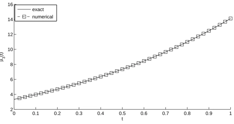
The numerical and the exact solution for the interior solution are shown in Figure 1 and one can notice that a very good agreement is obtained because the direct problem is well-posed. Figure 2 shows the numerical solution in comparison with exact one for µ3.

The trapezoidal rule is employed to compute the integral in (4) based on the formula

∫ 1

0

v(y, tj)dy=

1 2M

(

µ1(tj) +µ2(tj) + 2 M−1

∑

i=1

v(yi, tj)

)

From this figure it can be seen that the numerical solution is in excellent agreement with the exact one.

0 0.5

1

0 0.5 1 0 5 10 15

y Exact solution

t

exact

0 0.5

1

0 0.5 1 0 5 10 15

y Numerical solution

t

v(x,t)

0 0.5

1

0 0.5 1 0 0.2 0.4 0.6 0.8 1

x 10−3

y Absolute error

t

Absolute error

Figure 1: Exact and numerical solutions forv(y, t) and the absolute error for the direct problem obtained withM =N = 40.

0 0.1 0.2 0.3 0.4 0.5 0.6 0.7 0.8 0.9 1

2 4 6 8 10 12 14 16

µ 3

(t)

t exact

numerical

Figure 2: Exact and numerical integration for µ3(t) for the direct problem obtained with

4

Numerical Approach to the Inverse Problem

In the inverse problem, we assume that the free boundaryh(t) is unknown. The nonlinear inverse problem (6)–(9) can be reformulated as a nonlinear least-squares minimization of

F(h) =

h(t)

∫ 1

0

v(y, t)dy−µ3(t) 2

L2

[0,T]

, (26)

defined over the set of admissible functions h∈Λad :={h∈C1[0, T]

h(0) =h₀, h(t)>0 fort∈[0, T]}. (27)

The discretization of (26) is

F(h) =

N

∑

j=1 [

hj

∫ 1

0

v(y, tj)dy−µ3(tj)

]2

, (28)

whereh= (hj)_j=1,N. As it will be seen from the numerical results presented and discussed

in the next section, it seems that there is no need to regularize the least-squares functional (26) by adding to it a Tikhonov penalty term of some norm ofh, the problem being rather stable with respect to noise added in the input dataµ3(t).

The minimization ofF subject to the physical constraintsh >0 is accomplished using the MATLAB toolbox routinelsqnonlin, which does not require supplying by the user the gradient of the objective function (28), [8]. This routine attempts to find a minimum of a scalar function of several variables, starting from an initial guess, subject to constraints and this generally is referred to as a constrained nonlinear optimization.

We take bounds for the positive h(t) say, we seek the components of the vector h in the interval (10−10_,103_{). We also take the parameters of the routine as follows:}

• Number of variables M =N = 40.

• Maximum number of iterations = 102_{×(number of variables).}

• Maximum number of objective function evaluations = 103_{×(number of variables).} • x Tolerance (xTol) = 10−10_.

• Function Tolerance (FunTol) = 10−10 .

• Nonlinear constraint tolerance = 10−6_.

In addition, when we solve the inverse problem we approximate

h′ (tj) =

h(tj)−h(tj−1)

∆t =

hj −hj−1

∆t , j = 1, N , (29) and we expressh′

0 :=h

′

(0) as in (5). If there is noise in the measured data (4), we replace µ3(tj) in (28) by µϵ3(tj) given by

whereϵj are random variables generated from a Gaussian normal distribution with mean

zero and standard deviation σ, given by

σ =p× max

t∈[0,T]|µ3(t)|, (31)

where p represents the percentage of noise. We use the MATLAB function normrnd to generate the random variablesϵ= (ϵj)_j=1,N as follows:

ϵ=normrnd(0, σ, N). (32)

5

Numerical Results and Discussion

In this section, we will describe the numerical results for our nonlinear inverse problem for two different example according to the linear and nonlinear (rational) variation of free boundary. Moreover, we add noise to the measured input data (9) to mimic the reality situation by using (30) via (32). To compute this coefficient we use thelsqnonlinroutine combined with Trust-Region-reflective algorithm [8] to find the minimizer of the nonlinear functional (28). We also calculate the root mean square error (rmse) to analyse the error between the exact and numerically obtained coefficient, defined as,

rmse(h(t)) =

v u u t

1 N

N

∑

j=1

(hnumerical(tj)−hexact(tj))2. (33)

For simplicity, we takeT = 1 and the initial guess h(0) = 1 for all examples.

Example 1

Consider the problem (1)–(4) with unknown coefficienth(t), and solve this inverse problem with the following input data:

ϕ(x) = (1 +x)2+ 1, µ1(t) = 1 +et, µ2(t) = (2 +t)2+et,

µ3(t) =

(2 +t)3

3 + (1 +t)e

t₋ 1

3, a(u) = e −u_,

f(x, t) = et+e−(1+x)2 −et

(4x2+ 8x+ 2), h0 = 1,

One can remark that the conditions of Theorems 1 and 2 are satisfied hence, the existence and uniqueness of solution hold. With this data the analytical solution of inverse problem (1)–(4) is given by

h(t) = 1 +t, u(x, t) = (1 +x)2+et. (34) Then

We consider the case where there is no noise, i.e. p = 0, and when there is p = 2% noise in the input data (9).

The functional (28), as a function of the number of iterations, is represented in Fig-ure 3. From this figFig-ure it can be seen that the convergence is very fast in five and seven iterations for p = 0 and p = 2%, respectively. The objective function (28) decreases rapidly and takes a stationary value of O(10−7_{) and 0.3411, for p = 0 and p = 2%,}

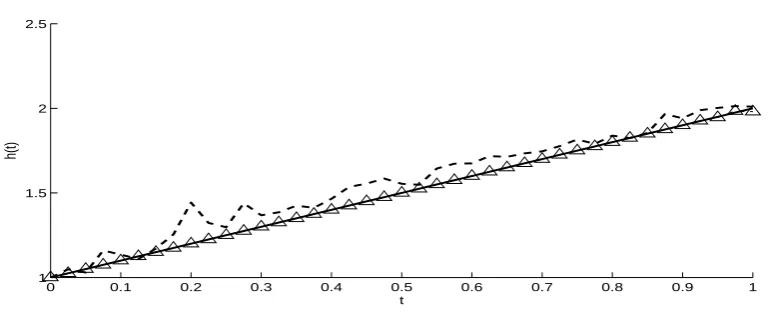
re-spectively. The numerical results for the corresponding unknown free boundary h(t) are presented in Figure 4. From this figure it can be seen that the retrieved free boundary h(t) is in very good agreement with the exact one in the case where no noise in the input data. While, when the input data is contaminated byp= 2% noise then we can see that the retrieved solution is stable and within the same range of errors as the input data is.

0 1 2 3 4 5 6 7

10−8 10−6 10−4 10−2 100 102 104

Number of Iterations

Objective function

Figure 3: Objective function (28) without noise (—), and forp= 2% noise (- - -) for Example

1.

0 0.1 0.2 0.3 0.4 0.5 0.6 0.7 0.8 0.9 1 1

1.5 2 2.5

t

h(t)

Figure 4: Free boundary h(t), without noise (-△-), and for_p= 2% noise (_{- - -}) in comparison with the exact solution (—), for Example 1.

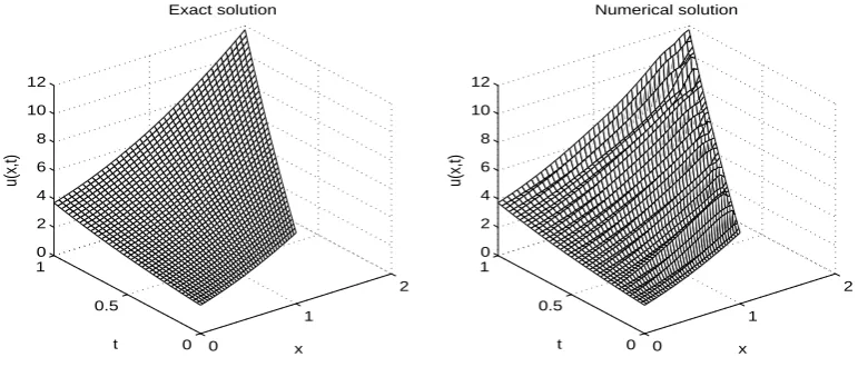
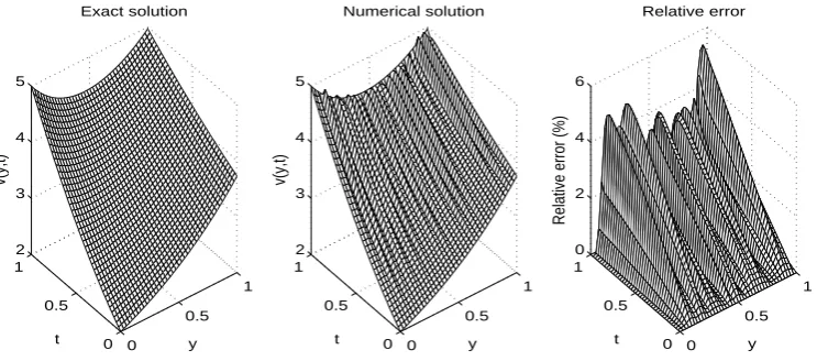
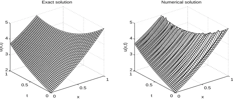
The restored temperatures v(y, t) and u(x, t) for p = 2% noise are shown in Figures 5 and 6, respectively. From these figures it can be seen that the solutions are stable by being free of high oscillations and unbounded behaviour.

stable with respect to noise in the input data for both the free boundary h(t) and the temperature/concentrationv(y, t) or u(x, t).

0 0.5 1 0 0.5 1 0 5 10 15 y Exact solution t v(y,t) 0 0.5 1 0 0.5 1 0 5 10 15 y Numerical solution t v(y,t) 0 0.5 1 0 0.5 1 0 5 10 15 20 y Relative error t

Relative error (%)

Figure 5: The analytical and numerical solutions, and the relative error for v(y, t) for p= 2% noise for Example 1.

0 1 2 0 0.5 1 0 2 4 6 8 10 12 x Exact solution t u(x,t) 0 1 2 0 0.5 1 0 2 4 6 8 10 12 x Numerical solution t u(x,t)

Figure 6: The analytical and numerical solutions for u(x, t) for p= 2% noise for Example 1.

Example 2

In this example, we consider a more severe test case where the unknown function h(t) is nonlinear with the following data

ϕ(x) = (1 +x)2 + 1, µ1(t) = 1 +et, µ2(t) = (

2 +t 1 +t

)2

+et_,

µ3(t) =

1 3

(

2 +t 1 +t

)3

+ e

t

1 +t − 1

3, a(u) = e −u_,

f(x, t) =et+e−(1+x)2 −et₍

4x2+ 8x+ 2)

, h0 = 1.

problem (1)–(4) is given by

h(t) = 1

1 +t, u(x, t) = (1 +x)

2_+et_{. (36)}

Then

h(t) = 1

1 +t, v(y, t) = u(yh(t), t) =

(

1 + y 1 +t

)2

+et_{, (37)}

is the analytical solution of the problem (6)–(9).

We study the case of exact and noisy input data (9). The objective function (28), as a function of the number of iterations is presented in Figure 7. From this figure it can be seen that the functional decreases very fast to stationary value at O(10−7_{) and 0.0188 in}

about 7 and 12 iterations, for p= 0 andp= 2% noise, respectively.

0 2 4 6 8 10 12

10−8 10−6 10−4 10−2 100 102 104

Number of Iterations

Objective function

Figure 7: Objective function (28) without noise (—), and forp= 2% noise (- - -) for Example

2.

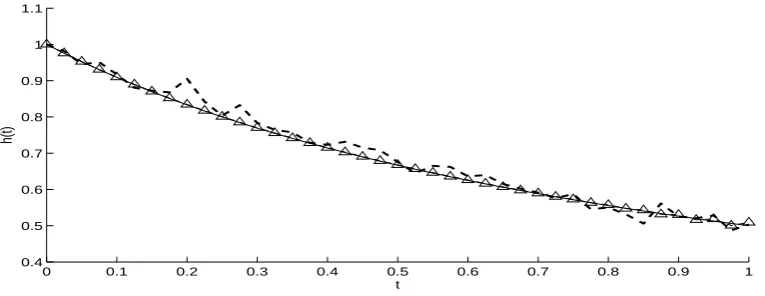
The numerical results for the corresponding free boundaryh(t) are presented in Figure 8. From this figure it can be seen that the identified free boundary is in very good agreement with the exact one in the absence of noise and this situation changes only a little when we perturb the input data by p= 2% noise.

0 0.1 0.2 0.3 0.4 0.5 0.6 0.7 0.8 0.9 1 0.4

0.5 0.6 0.7 0.8 0.9 1 1.1

t

h(t)

The numerical solutions for v(y, t) and u(x, t) are shown in Figure 9 and 10, respec-tively, in comparison with the exact solutions forp= 2% noise. As in Example 1, stable numerical solutions are obtained.

One can conclude that the inverse problem is well-posed since small errors in the measurement in (4) cause only small errors in the retrieved pair solution (h(t), u(x, t)). Consequently, we can say that the problem depends continuously on the input data.

Finally, for completeness, other details about the number of iterations, number of function evaluations, objective function value at final iteration andrmse(h) for Examples 1 and 2 are given in Table 1. For this table it can be seen that accurate and stable numer-ical solutions are rapidly achieved by the iterative MATLAB toolbox routine lsqnonlin.

Table 1: Number of iterations, number of function evaluations, value of the objective function (28) at final iteration andrmse values (33), for Examples 1 and 2.

p= 0 p= 2%

Example 1

No. of iterations 5 7

No. of function evaluations 252 336 Function value at final iteration 2E−7 0.3411 rmse(h) 0.0035 0.0793

Example 2

No. of iterations 7 12

No. of function evaluations 336 546 Function value at final iteration 6E−7 0.0188 rmse(h) 0.0023 0.0212

0 0.5

1

0 0.5 1 2 3 4 5

y Exact solution

t

v(y,t)

0 0.5

1

0 0.5 1 2 3 4 5

y Numerical solution

t

v(y,t)

0 0.5

1

0 0.5 1 0 2 4 6

y Relative error

t

Relative error (%)

0

0.5

1

0 0.5 1 2 3 4 5

x Exact solution

t

u(x,t)

0

0.5

1

0 0.5 1 2 3 4 5

x Numerical solution

t

u(x,t)

Figure 10: The analytical and numerical solutions foru(x, t) for p= 2% noise for Example 2.

6

Conclusions

The inverse problem concerning the identification of free boundaryh(t) and the temper-ature u(x, t) in the heat equation with nonlinear diffusivity a(u) has been investigated. The additional condition which ensures a unique solution is given by the energy/mass specification µ3(t) given by equation (4). As with other free surface problems, it turns

out that the problem is well-posed if the dataµ3 is smooth. The direct solver based on a

three-level finite difference scheme is developed. The inverse solver is based on a nonlinear least-squares minimization which is solved using the MATLAB toolbox routinelsqnonlin. As expected, for exact data, the numerical results obtained are very accurate. For noisy dataµϵ

3 which consist of a random perturbation of the exact data µ3, the results forh(t),

v(y, t) and u(x, t) are still stable and accurate. The instability is only manifested in the derivativeh′

(t) for which the use of a regularization method would be warranted.

Acknowledgments

M.S. Hussein would like to thank the Higher Committee of Education Development in Iraq (HCEDiraq) for their financial support in this research.

References

[1] Broadbridge, P., Tritscher, P. and Avagliano, A. (1993) Free boundary problems with nonlinear diffusion,Mathematical and Computer Modelling, 18, 15–34.

[2] Cannon, J.R. and Duchateau, P. (1973) Determining unknown coefficients in a non-linear heat conduction problem,SIAM Journal on Applied Mathematics,24, 298–314. [3] Cannon, J.R. and Duchateau, P. (1980) An inverse problem for a nonlinear diffusion

equation,SIAM Journal on Applied Mathematics, 39, 272–289.

[4] Cannon, J.R. and Hoek, J. (1986) Diffusion subject to the specification of mass,

[5] Friedman, A. (1964) Partial Differential Equations of Parabolic Type, Prentice-Hall, Englewood Cliffs, NJ.

[6] Ivanchov, M.I. (2003) Free boundary problem for nonlinear diffusion equation,

Matematychni Studii, 19, 156-164.

[7] Lees, M. (1966) A linear three-level difference scheme for quasilinear parabolic equa-tions, Mathematics of Computation, 20, 516–522.

[8] Mathworks R2012 Documentation Optimization Toolbox-Least Squares (Model Fit-ting) Algorithms, available from www.mathworks.com/help/toolbox/optim/ug /brnoybu.html.

[9] Murio, D.A.(1993) The Mollification Method and the Numerical Solution of Ill-posed Probelms, Wiley, New York.

[10] Smith, G.D. (1985)Numerical Solution of Partial Differential Equations: Finite Dif-ference Methods, Oxford Applied Mathematics and Computing Science Series, Third Edition.