Influence of a velocity model and source frequency on microseismic waveforms: some implications for microseismic locations

promoting access to White Rose research papers

White Rose Research Online

[email protected]

Universities of Leeds, Sheffield and York

http://eprints.whiterose.ac.uk/

This is an author produced version of a paper published in

Geophysical

Prospecting

White Rose Research Online URL for this paper:

http://eprints.whiterose.ac.uk/id/eprint/77376

Paper:

Usher, PJ, Angus, DA and Verdon, JP (2013)

Influence of a velocity model and

source frequency on microseismic waveforms: some implications for

microseismic locations.

Geophysical Prospecting, 61 (Supple). 334 - 345 (12).

ISSN 0016-8025

microseismic waveforms: some implications for

microseismic locations

P.J. Usher

, D.A. Angus

& J.P. Verdon

1

Department of Earth Sciences, University of Bristol, Bristol, UK

2

CiPEG, University of Leeds, Leeds, UK

3

School of Earth & Environment, University of Leeds, Leeds, UK

Submitted to Geophysical Prospecting: 2011

Key words: microseismicity, source frequency, velocity model, waveforms.

Abstract

In this paper, we examine the influence of velocity model and microseismic source frequency on microseismic waveforms and event locations. Finite–difference waveform synthetics are generated based on the Cotton Valley hydraulic fracture experiment, where we vary the vertical heterogeneity of the velocity models as well as the microseis-mic source frequencies. We find that differences between plausible velocity models lead to changes in arrival times of approximately 0.0035 seconds for P–waves and 0.0085 seconds for S–waves. Based on the average P– and S–wave velocities, the difference in P– and S–wave travel times is equivalent to approximately 20 m in location difference. Significant increases in waveform coda develop with increasing model heterogeneity and increasing source frequency. The presence of signal noise as well as other sources of error (e.g., uncertainty in geophone location) will likely lead to further increase in uncertainty in location error estimates. Thus we note that location error due to incorrect velocity models cannot be ignored.

1 INTRODUCTION

Microseismicity is ideally suited and actively used to study the state of stress and fracturing in rock mass (e.g., Gibow-icz and Kijko, 1994). Monitoring the distribution of micro-seismic attributes (e.g., event location and source mecha-nism) in space and in time provides insight into the spa-tial and temporal variations in the stress field, and is com-monly used to delineate activity on pre–existing faults and joint systems as well as identify their orientation and den-sity. Hence, over the past couple of decades, microseismic monitoring has become increasingly common in the hydro-carbon industry as a tool to investigate production related geomechanical deformation (such as subsidence, e.g. Dyer et al., 1999) as well as audit hydraulic fracture stimulation treatments (e.g., Maxwell and Urbancic, 2005). Waveform attributes, such as amplitude and polarity, can be used to invert for the failure mechanisms (e.g., moment tensors) of both pre–existing and newly generated fractures or fracture systems (e.g., Baig and Urbancic, 2010), as well as evaluate the fracture stimulation program (e.g., Baig et al., 2011). As a passive source, microseismicity can be used to charac-terize spatial and temporal variations in seismic attributes (e.g., seismic anisotropy) within the rock mass between the

source and receiver (e.g., see Verdon and Kendall, 2011, for estimating fracture orientation and density).

2

P.J. Usher, D.A. Angus & J.P. Verdon

thorough discussion on the importance of location accuracy and the necessity of reliably quantifying location error.

Location errors stem from limitations due to monitoring array geometry (e.g., Eisner et al., 2009; Jansky et al., 2010) as well as uncertainty in traveltime picks (e.g., Eisner et al., 2010), event azimuths (e.g. Jones et al., 2010) and velocity model. Probably least well understood is the impact of veloc-ity model error on location accuracy. In this paper, we study the influence of velocity model and source frequency on microseismic waveforms and explore how these parameters might influence location. To do this, we generate synthetic waveform data using the finite–difference method to assess the impact of frequency dependence of seismic waveforms due to velocity model heterogeneity. Although the influence of velocity model heterogeneity on band–limited waveforms seems intuitive (e.g., Angus, 2005), finite–frequency effects are often overlooked in location error studies. For instance, although ray based approaches (i.e., high frequency asymp-totic solutions) provide valuable contributions to our under-standing of velocity models and locations (e.g., Eisner et al., 2009), they do not consider the influence of velocity varia-tions on the order of or less than the seismic wavelength. To facilitate comparison with observed microseismic wave-forms and hence help provide qualitative justification for our synthetic study, the synthetic model used in this study is based on the Cotton Valley hydraulic fracture experiment (see Walker, 1997; Rutledge et al., 2004).

2 MICROSEISMIC LOCATION

The location of a microseismic event tells us where and when the rock mass is undergoing elastic failure. For instance, if we consider the case of hydraulic fracture stimulation, mi-croseismic event location provides a means to monitor and potentially manage the geometry of stimulated fractures. If the fracturing progresses outside the perforation or injection interval (e.g., reservoir bed), this can have important eco-nomical and environmental consequences, either in terms of loss of hydrocarbon or leakage of CO2. As well, monitoring the number of events within each bed can be used to quan-tify the seismic injection efficiency of each bed (Maxwell et al., 2008). Thus, improving location accuracy will lead to higher resolution imaging of features. Furthermore, any er-ror associated with event location will be passed on to any subsequent interpretation and/or estimates of other micro-seismic attributes, such as source mechanism (e.g., Angus, 1998) or seismic anisotropy (e.g., Verdon and Kendall, 2011). There are three main techniques for locating microseis-mic events (Maxwell et al., 2010a): triangulation, hodogram and semblance based techniques. The triangulation tech-nique uses P–wave and/or S–wave arrival time picks from numerous stations to locate microseismicity. The event time and spatial location can be estimated using arrival time phase picks and a velocity model. The hodogram technique uses the particle motion of the P–wave phase, where the par-ticle motion is polarized along the direction of wave propa-gation. From the particle motion, the azimuth to the earth-quake can be found. For single–station or single–borehole arrays, there is a 180◦_{ambiguity in azimuth and}

incorpora-tion of dip is often needed (e.g., Jones et al., 2010). For the hodogram approach, travel time phase picks and a velocity

model are required. The semblance technique (e.g., Duncan and Eisner, 2010) is similar to migration and involves propa-gating the microseismic energy back to its hypocenter using a Green’s function (e.g., Kirchhoff, Gaussian beam and one– way wave equation migration) and does not require arrival time phase picks (e.g., Rentsch et al., 2007; Duncan and Eisner, 2010). It is important to stress that in all three ap-proaches a velocity model is required. Yet the velocity model may be poorly constrained and is often neglected within lo-cation error analysis.

Over the past several decades there have been a variety of studies that have explored the quantification of location error. For instance, Pavlis (1986) looked at the combination of different sources of error on location accuracy, including source–receiver geometry, velocity model and phase picking. In general, error analysis considers only the misfit between the observed and predicted data using what is assumed to be a well known velocity model (e.g., Zimmer et al., 2007). It is generally, yet incorrectly, interpreted that as the es-timation of location error approaches zero, the estimated event location approaches that of the true event location. More recently, however, the influence of velocity model on location has been given greater consideration (e.g., Eisner et al., 2009; Maxwell, 2009). For instance, Urbancic et al. (2009) provide a statistical estimate of event location using confidence limits and is similar to the approach developed by Foulger and Julian (2012) for geothermal applications. Yet few of these studies consider the influence of velocity model on band–limited seismic waveforms, where even weak heterogeneity can significantly influence seismic waveforms and wavefronts (e.g., Angus, 2005).

3 VELOCITY MODEL

There are many different types of velocity model available for a reservoir. Active–source surface seismic surveys provide large volume maps of the reservoir, but have relatively low vertical and horizontal resolution. On the scale of hydraulic stimulation, the sub–volume of stimulated rock mass may appear relatively homogeneous within surface seismic veloc-ity models. Vertical seismic profile (VSP) surveys generally provide higher spatial resolution (predominantly vertical) than active surface seismics, but at a loss of horizontal spa-tial sampling (i.e., velocity model becomes more localized around the borehole). Sonic velocity logs provide the high-est resolution in terms of vertical structure, but very little if any lateral information. The choice of velocity model in mi-croseismic event location depends on availability, how well it performs in locating calibration shots and the array geome-try. Often, a velocity model might be modified to ensure that perforation shots, which have a known location, are located accurately.

Figure 1.Top: sonic velocity log (blue) and filtered version (red) for well CGU 21-10. Bottom: synthetic P- and S-wave velocity models for Cotton Valley hydraulic experiment; surface seismic model (blue), VSP model (black) and sonic model (red).

along grids on the surface, or placed in shallow boreholes (typically 50-200m) to reduce surface noise and higher atten-uation in near-surface layers. As surface arrays are located further away from the event hypocenters in comparison to borehole arrays, microseismic waveforms recorded at the sur-face suffer from a low signal–to–noise ratio due to geomet-rical spreading and attenuation. Thus surface microseismic monitoring often requires waveform stacking (e.g., Duncan and Eisner, 2010) and migration based location techniques (e.g., Chambers et al., 2010). Surface seismic and/or VSP type velocity models may therefore be more suitable for sur-face seismic location processing.

Given the range of velocity models with differing spa-tial resolution, an informed choice in the velocity model used in locating microseismicity is required, and a better under-standing of the influence of velocity model on location error is advisable. For hydraulic stimulation, sonic velocity mod-els are commonly used to locate microseismic events (see Maxwell et al., 1998, and others). Sonic velocity models are ideal primarily due to their availability as well as the fact that the sonic frequencies (e.g., up to 2 kHz, Bulant and Klimeˇs, 2008) are within the upper range of typical micro-seismic events (e.g., 10’s to 100’s of Hz). However, lithology plays an important role, where it has been observed that in certain settings the velocity contrasts are relatively weak

such that a smooth model is sufficient, and in other settings the velocity contrasts are severe enough that headwaves are pervasive and problematic such that a smooth model is likely insufficient (Zimmer, 2011, personal communication).

In this study, we synthesize three velocity models to mimic the types of velocity model that can be generated from a surface seismic survey, a VSP survey and a sonic log using data from the Cotton Valley, East Texas Basin, U.S., hydraulic fracture experiment (see Walker, 1997). The main reason for choosing Cotton Valley is because it has been ex-tensively studied (see Rutledge et al., 2004, and references therein) and allows for direct comparison with observed mi-croseismic waveforms. Cotton Valley is a tight–gas reservoir and hence has low permeability. Therefore it has undergone two stages of hydraulic stimulation: an injection stage using a gel treatment and an injection stage using a water treat-ment. The microseismic activity is located approximately at a depth of 2.5 km and so we limit our synthetic veloc-ity models (and simulations) to within the depth range of 2 and 3 km. We use the sonic velocity log data from the well located closest to the injection point (well CGU 21-10) to derive our synthetic VSP and sonic velocity models. This log contains both P– and S–wave sonic velocity data.

Figure 1 displays the sonic log and the three synthetic velocity models derived for our synthetic study. Based on numerical consideration (microseismic source frequency and finite–difference dispersion criteria discussed in the follow-ing section), the sonic velocity log for well CGU 21-10 was decimated to a 34 layer model (layer thickness of approx-imately 30 m). O’Brien and Harris (2006) provide a VSP model for Cotton Valley, but only to depth shallower than the region of interest. Thus, the constructed VSP model for this study was aided by the observed characteristics pro-vided by O’Brien and Harris (2006). The VSP model is de-fined by 13 discrete layers consistent with the derived sonic log (layer thickness on the order of 75 m). The surface seis-mic velocity model is based on the three–layer model used by Rutledge and Phillips (2003).

4 MICROSEISMIC WAVEFORM MODELLING

sen-4

P.J. Usher, D.A. Angus & J.P. Verdon

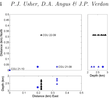
Figure 2.Location of the boreholes in map view (top) and the location of the geophones (triangles) in cross section (right and bottom). The location of the modelled source is indicated by the star. The two monitoring boreholes CGU 22-09 and CGU 21-09 are labeled as well as the injector well CGU 21-10.

sitivity and coupling of the instrumentation, the presence of background noise (e.g., operational noise), and path effects (e.g., attenuation).

Assuming P– and S–wave velocities 4750 m/s and 3000 m/s, respectively, a 40 Hz microseismic event will have dom-inant wavelength on the order of 100 m whereas a 150 Hz microseismic event will have wavelength of 30 m. If the true velocity model has velocity heterogeneity on the order of 100 m or less, frequency–dependent waveform effects will be sig-nificant (Angus, 2005). For such a scenario, ray theoretical approaches may be neglecting important wave phenomena and hence full waveforms synthetics may be needed to cap-ture frequency–dependent effects. However, full waveform synthetic studies have rarely been performed, most likely be-cause full waveform algorithms, such as the finite–difference method, can be computationally expensive.

In this study, we use the full waveform E3D code (Larsen and Harris, 1993) to generate synthetic waveforms. E3D is a staggered grid, fourth–order accurate in space and second–order accurate in time finite–difference algorithm for isotropic two–dimensional (2D) and three–dimensional (3D) viscoelastic media. It has been used recently to model micro-seismicity in hard–rock mining applications to benchmark an automated event location algorithm (Gharti et al., 2010) and this study was the impetus for using E3D to examine microseismic waveform effects. The synthetic microseismic sources and reservoir model were designed to mimic the Cot-ton Valley hydraulic fracture experiment (Walker, 1997) to enable us to qualitatively relate the numerical simulations to real observed microseismic data.

4.1 Microseismic source

There are over 800 recorded events in the Cotton Valley data set and so we selected a synthetic source location within the middle of the recorded seismicity (see asterisk between wells CGU 21-10 and CGU 21-09 in Figure 2). The location of the microseismic event is kept constant in all simulations

to focus solely on the influence of velocity model depen-dence as well as source frequency dependepen-dence in the syn-thetic waveforms. To be consistent with events recorded at Cotton Valley, the source parameters are derived from the inverted focal solutions of Rutledge et al. (2004), where the dominant source mechanism is strike–slip with approximate north–south, east–west striking nodal planes and dip of ap-proximately 85◦_.

As discussed earlier, the range of source frequencies can vary depending on several factors. In a previous study of Cotton Valley microseismicity, Rentsch et al. (2007) observe a dominant frequency of 100 Hz. It is not uncommon, how-ever, to observe dominant frequencies down to the 10’s of Hz (e.g., Teanby et al., 2004) and up to the 100’s Hz (e.g., Trifu et al., 2000). Therefore, to capture a realistic range of source frequencies, we simulate three source frequencies at 40 Hz, 150 Hz and 300 Hz. Based on Urbancic and Zinno (1998), we define the microseismic moment magnitude to be 4.4×1010

dyne.cm for all source frequencies. We keep the size of the seismic moment constant in all simulations to facil-itate waveform comparisons, but note here that the source moment magnitude would be smaller for higher dominant frequency sources and larger for lower dominant frequency sources (e.g., see Izutani and Kanamori, 2001, Figure 4). For most microseismic analysis (with the exception of rock-burst studies in mining), the elastic medium is linear elastic and hence differences in source moment magnitude trans-lates into differences in waveform amplitude and not shape (e.g., Liner, 2004).

4.2 Model geometry

The locations of the model geophone arrays and the syn-thetic microseismic source are shown in Figure 2. This is based on the field configuration shown in Figure 1 of Rut-ledge et al. (2004). For the simulations, we assume that the geophone arrays are vertical (i.e., no lateral borehole devi-ation). For the gel treatment (i.e., the second stage of in-jection), the injector well is CGU 21-10 and the monitoring arrays are CGU 22-09 and CGU 21-09 (with average vertical geophone spacing of 70 m). Array CGU 22-09 consists of 10 working geophones, whereas CGU 21-09 consists of 3 work-ing geophones. For the water treatment (i.e., the first stage of injection), the injection well is CGU 21-09 and only the single borehole array CGU 22-09 is used to record micro-seismicity. To model the microseismic waveforms of the gel treatment, the multiple arrays were modelled as two sep-arate 2D vertical profiles (e.g., vertical plane through the source and respective borehole array).

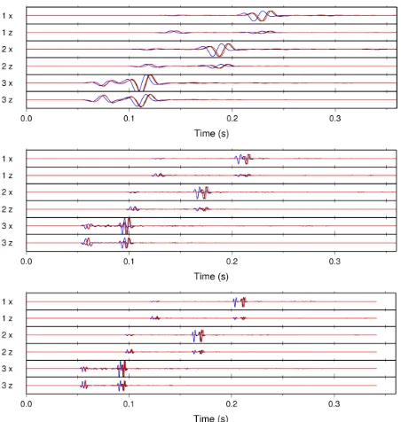
Figure 3.Comparison of 40 Hz waveforms for the surface seismic (blue), VSP (black) and sonic (red) velocity models.

and in 2D is proportional to 1/√r). Thus, if significant lat-eral heterogeneity is expected or if absolute amplitudes are required (e.g., for moment tensor analysis), full 3D simula-tion would be necessary.

In all simulations, the model has a lateral extent of 5000 m and a vertical extent of 1000 m. The density of the model is constant throughout at 3000 kg/m3

. Since we are mod-elling a sub–volume at depth, all four boundaries are set as absorbing boundaries (Clayton and Engquist, 1977). To minimize numerical dispersion, satisfy numerical stability and maintain computational efficiency, the grid and time parameters for all source frequencies vary. Specifically, we define the grid increment ∆hsuch that we have at least 10 grid points per minimum wavelengthλmin, ∆h=λmin/10 (e.g., Alford et al., 1974), and define the time increment ∆t

such that the relationship ∆t_≤0.606∆h/Vmax holds, (e.g., Kelly et al., 1976)], where Vmax is the maximum velocity. For the 40 Hz source, the grid spacing is 6 m with time in-crement 0.6 ms and total time samples of 600. For the 150 Hz source, the grid spacing is reduced to 1 m with time in-crement of 0.1 ms and total time samples of 3600. For the 300 Hz source, the grid spacing required is 0.5 m with time increment of 0.056 ms and 6100 time samples.

5 SYNTHETIC WAVEFORM RESULTS

To increase our understanding of the influence of velocity model on microseismic waveforms and implications for mi-croseismic locations, we generate synthetic waveforms while varying the velocity model, the microseismic source fre-quency, and the array geometry (specifically geophone prox-imity). For most of the simulations, we model the single ar-ray CGU 22-09 because it consists of ten geophones and al-lows for greater waveform comparison. Since all simulations are 2D, the synthetic traces have horizontal (x) component and vertical (z) component. All trace amplitudes are nor-malized to the largest amplitude within the geophone array.

5.1 Sensitivity to velocity model

To compare the influence of velocity models, we simulate three microseismic events with a double–couple source hav-ing strike 80◦_{and dip 85}◦_{, and source frequencies of 40 Hz,}

150 Hz and 300 Hz, respectively. The results for each velocity

Figure 4.Comparison of 150 Hz waveforms for the surface seis-mic (blue), VSP (black) and sonic (red) velocity models.

Figure 5.Comparison of 300 Hz waveforms for the surface seis-mic (blue), VSP (black) and sonic (red) velocity models.

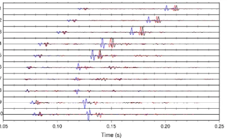
model are shown in Figure 3 for the 40Hz case, in Figure 4 for the 150Hz case, and in Figure 5 for the 300Hz case. There are several observations that can be made when comparing Figures 3–5. First, the P–wave phase arrivals for all velocity models at 40 Hz are approximately equal for geophones 6– 8. This is because the ray paths are horizontal and at this low frequency the velocity models for this depth interval are roughly equivalent (i.e., the vertical heterogeneity of the VSP and sonic velocity model are averaged over the approx-imate 100 m dominant seismic wavelength). As the source frequency increases, the Pwave phase arrivals for geophones 6–8 begin to deviate as the influence of material averaging decreases (i.e., dominant wavelength decreases). Second, for all cases the S–wave phase arrivals differ and this is particu-larly significant for the surface seismic velocity model. This suggests that the Vp/Vsratios for each layer in the surface seismic model do not represent consistent Vp/Vsratios with respect to the VSP and sonic velocity models. Third, as the frequency of the source increases so does the coda and this is expected as the shorter wavelength signals are scattered to a much greater degree. Finally, there are noticeable differences between the P– and S–wave phase separation times. This ob-servation may significantly impact location algorithms that are based on the differential P– and S–wave travel times.

6

P.J. Usher, D.A. Angus & J.P. Verdon

Figure 6.Cross correlation for the sonic velocity model (blue) and the VSP velocity model (black) at 300Hz against the surface seismic velocity model: (top) P–wave phase and (bottom) S–wave phase. All the traces show a clear maximum peak which is the delay with respect to the surface seismic velocity model.

wave and S–wave phases. We use the surface seismic velocity model synthetics as the reference time series and perform cross correlation on the VSP and sonic velocity model syn-thetics for each geophone. Figure 6 displays the cross cor-relation for the P– and S–wave phases between the surface seismic and VSP velocity models, and the surface seismic and the sonic velocity models. The maximum cross correla-tion gives the travel time difference for the particular phase (P–wave or S–wave) between the velocity models. Table 1 summarizes the results for the 300 Hz source event. The mean P–wave phase shift is 3.5 ms for the VSP velocity model and 3.6 ms for the sonic velocity model. The mean S–wave phase shift is higher, with 8.4 ms for the VSP ve-locity model and 8.5 ms for the sonic veve-locity model. For P– and S–wave velocities of 5000 m/s and 3000 m/s, the arrival time differences are equivalent to approximately 20 m in location.

It should be noted that some of the S–wave cross cor-relations for geophones 6, 7 and 8 have unrealistically large values (denoted NA in Table 1). In Figures 3–5, it can be seen that the S–wave phases are distinctively different and uncorrelated. This is because the geophones for these traces are located within the minimum amplitude region of the S–wave radiation pattern for the modelled double–couple source mechanism (e.g., Lay and Wallace, 1995) and so the waveform amplitudes are very low. Thus the signals being correlated are non–primary arrivals. The results show that both the P– and S–wave phase arrivals vary not only be-tween velocity models but also with microseismic source fre-quency. The main differences due to the velocity model are changes in the arrival times, whereas the differences due to

VSP Sonic

Geophone P–wave (s) S–wave (s) P–wave (s) S–wave (s) 1 0.0049 0.0078 0.0056 0.0093 2 0.0049 0.0077 0.0054 0.0093 3 0.0052 0.0083 0.0058 0.0102 4 0.0054 0.0077 0.0058 0.0098 5 0.0041 0.0064 0.0043 0.0071

6 0.0012 NA 0.0007 NA

7 -0.0003 NA -0.0010 NA 8 -0.0002 NA -0.0003 0.0113 9 0.0052 0.0100 0.0037 0.0056 10 0.0054 0.0112 0.0048 0.0085

Table 1.P- and S-wave arrival time differences at 300Hz between the 3 layer model and the VSP-based model, and between the 3 layer model and the sonic log-based model. Note that no S-wave picks were possible on geophones 6,7 and 8 for the VSP-based model data, and geophones 6 and 7 for the sonic log-based model data.

Figure 7.Shows the waveforms for the sonic velocity model for varying frequencies 40Hz (top), 150Hz (middle), and 300Hz (bot-tom) from the other geophone array. Notice that the coda is less developed compared to the waveforms in well CGU 22-09.

frequency appear to be the strength of the coda as well as changes in travel times of the P– and S–wave phase. Thus the frequency dependence of coda could be used to assess the suitability of the velocity model.

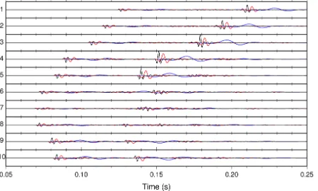
Figure 8. Shows the waveforms for the 40 Hz (blue), 150 Hz (black) and 300 Hz (red) source and the sonic velocity model. All the wavelets have similar first breaks however the main peak of the wave is delayed more with lower frequency.

in the waveforms from well CGU 22-09. However, the phase arrival differences discussed above are still present.

5.2 Sensitivity to source frequency

Having examined the dependence of arrival time on the choice of velocity model, we now examine the effects of source frequency on waveforms and arrival times. In Fig-ure 8, we plot the simulated waveforms generated using the sonic velocity model and a double–couple source with strike 80◦ _{and dip 85}◦_{, and source frequencies of 40 Hz, 150 Hz}

and 300 Hz. At 40 Hz frequency, the waveforms are less complex even within the highly heterogeneous sonic veloc-ity model. As the source frequency increases, the waveform complexity increases, with significant increase in coda. The lower frequencies have larger wavelengths and hence sample a larger velocity space, whereas the higher frequencies have smaller wavelengths are hence are much more sensitive to lo-cal velocity variations. Arrival time differences in the phase peaks are also observed in Figure 8. Focusing on the first break (the first deviation from zero amplitude), the P– and S–wave phases have essentially identical arrival times for all frequencies. However, in practice, ambient and instrument noise in real data would obscure identification of these first breaks.

6 DISCUSSION

Changes in the velocity model cause a systematic change in the arrival time as well as significant coda trailing the pri-mary P–wave phase. For certain environments, the litholog-ical contrast (even though highly heterogeneous in a petro-physical sense) could be so small that a smooth, weakly heterogenous velocity model is sufficient. Yet in other en-vironments, the elastic contrasts may be large enough that a strongly heterogeneous velocity model is required. With increasing source frequency, the influence of velocity model increases. This suggests it is important to consider the range of source frequencies of microseismic events as well as the strength of elastic contrasts due to lithology when construct-ing a velocity model for event location processconstruct-ing. Further-more, recent work in modelling microseismicity using

cou-pled flow–flow and geomechanical simulation (e.g., Angus et al., 2010; Zhao and Young, 2012) will require appropri-ate velocity models to bench mark predictions with micro-seismic waveform data. Thus an understanding of the influ-ence of velocity model on microseismic waveforms will guide any necessary modifications to the synthetic velocity models (e.g., spatial smoothing) used in generating synthetic micro-seismic waveforms.

The velocities models used show significant variations in velocity in the middle layers so one would expect the ar-rivals particularly at the central geophones in the array to be different. This is not always the case due to material averag-ing duraverag-ing wave propagation. In other words, the wavefield has finite-frequency and hence the wavefield is sensitive to a localized volume dependent on the frequency content of the signal rather than limited to an infinitesimal ray.

It is important to note that the variations of arrival times in P and S waves (3.5ms and 8.5ms respectively) will significantly effect location algorithms, unless errors associ-ated with the velocity model are taken into account. Cur-rently, calibration and perforation shots are typically used to benchmark the location algorithm and velocity model. Any location algorithm that does not take into account errors in velocity model and finite-frequency effects will significantly underestimate the location error. In essence, this is a fairly obvious observation and relates to the highly non–linear and non–unique characteristic of the location inversion problem.

7 CONCLUSION

We examine the importance of velocity model and micro-seismic source frequency on micromicro-seismic waveforms using finite–difference waveform synthetics. We simulate wave-forms for a source–receiver geometry typical of hydraulic fracture programs. Specifically, we model a multilevel bore-hole array of receivers using a source located horizontally from the array with distance on the order of a few hundred meters. The variations in velocity models manifest in per-turbations in arrival times of the P– and S–wave phases of approximately 3.5 ms and 8.5 ms, respectively. The differ-ences in arrival times are equivalent to approximately 20 m in location. As the model heterogeneity and the source frequency increase, the strength of the waveform coda in-creases.

8 ACKNOWLEDGEMENTS

We would like to thank James Rutledge for providing the well logs and velocity models for the Cotton Valley hy-draulic experiment and members of the BUMPS consortium for helpful discussion of the waveform modelling results.

References

Alford, R., Kelly, K., and Boore, D., 1974, Accuracy of finite–difference modeling of the acoustic wave equation: Geophysics,39, no. 6, 834–842.

8

P.J. Usher, D.A. Angus & J.P. Verdon

Skachkov, S., Crook, A. J. L., and Dutko, M., 2010, Mod-elling microseismicity of a producing reservoir from cou-pled fluid-flow and geomechanical simulation: Geophysical Prospecting,58, 901–914.

Angus, D. A., 1998, Applicability of moment tensor inver-sions to mine–induced microseismic data: Master’s thesis, Queen’s University, Canada.

Angus, D. A., 2005, A one–way wave equation for modelling seismic waveform variations due to elastic heterogeneity: Geophysical Journal International,162, 882–898. Baig, A., and Urbancic, T.-I., 2010, Microseismic moment

tensors: A path to understanding frac growth: The Lead-ing Edge,29, no. 3, 320–324.

Baig, A. M., Urbancic, T.-I., Guest, A., von Lunen, E., and Hendrick, J., 2011, Evaluating the effectiveness of hy-draulic fracture staging with moment tensors: Recovery: 2011 CSPG CSEG CWLS Convention.

Bulant, P., and Klimeˇs, L., 2008, Comparison of vsp and sonic-log data in nonvertical wells in a heterogeneous structure: Geophysics,73, no. 4, U19–U25.

Chambers, K., Kendall, J.-M., Brandsberg-Dahl, S., and Rueda, J., 2010, Testing the ability of surface arrays to monitor microseismic activity: Geophysical Prospecting,

58, no. 5, 817–826.

Clayton, R., and Engquist, B., 1977, Absorbing boundary conditions for acoustic and elastic wave equations: Bul-letin of the Seismological Society of America, 67, no. 6, 1529–1540.

Duncan, P., and Eisner, L., 2010, Reservoir characteriza-tion using surface microseismic monitoring: Geophysics,

75, no. 5.

Dyer, B., Jones, R., Cowles, J., Barkved, O., and Folstad, P., 1999, Microseismic survey of a north sea reservoir: World Oil,220, no. 3, 74–78.

Eisner, L., Duncan, P. M., Heigl, W. M., and Keller, W. R., 2009, Uncertainties in passive seismic monitoring: The Leading Edge,28, no. 6, 648–655.

Eisner, L., Hulsey, B. J., Duncan, P., Jurick, D., Heigl, W., and Keller, W., 2010, Comparison of surface and borehole locations of induced seismicity: Geophysical Prospecting,

58, no. 5, 805–816.

Foulger, J., and Julian, B., 2012, Earthquakes and errors: methods for industrial applications: Geophysics, 76, no. 6, WC5–WC15.

Gharti, H. N., Oye, V., Roth, M., and Kuhn, D., 2010, Au-tomated microearthquake location using envelope stack-ing and robust global optimization: Geophysics, 75, no. 4, MA27–MA46.

Gibowicz, S. J., and Kijko, A., 1994, An introduction to mining seismology: Academic Press.

Izutani, Y., and Kanamori, H., 2001, Scale–dependence of seismic energy–to–moment ratio for strike–slip earth-quakes in japan: Geophysical Research Letters, 28, no. 20, 4007–4010.

Jansky, J., Plicka, V., and Eisner, L., 2010, Feasibility of joint 1D velocity model and event location inversion by the Neighbourhood algorithm: Geophysical Prospecting,

58, no. 2, 229–234.

Jones, G. A., Raymer, D., Chambers, K., and Kendall, J.-M., 2010, Improved microseismic event location by inclu-sion of a priori dip particle motion: a case study from Ekofisk: Geophysical Prospecting,58, no. 5, 727–737.

Kelly, K., Ward, R., Treitel, S., and Alford, R. Synthetic seismograms: a finite–difference approach:, 1976.

Larsen, S., and Harris, D., 1993, Seismic wave propagation through a low-velocity nuclear rubble zone: Lawrence Liv-ermore National Lab.

Lay, T., and Wallace, T. C., 1995, Modern Global Seismol-ogy: Academic Press.

Liner, C. L., 2004, Elements of 3D seismology: PennWell. Maxwell, S. C., and Urbancic, T. I., 2005, The potential

role of passive seismic monitoring for real–time 4d reser-voir characterization: SPE Reserreser-voir Evaluation and En-gineering, pages 70–76.

Maxwell, S. C., Young, R. P., Bossu, R., Jupe, A., and Dangerfield, J., 1998, Microseismic Logging of the Ekofisk Reservoir: SPE/ISRM Rock Mechanics in Petroleum En-gineering Conference.

Maxwell, S., Shemeta, J., Campbell, E., and Quirk, D., 2008, Seismic deformation rate monitoring: SPE, page SPE134695.

Maxwell, S. C., Rutledge, J., Jones, R., and Fehler, M., 2010a, Petroleum reservoir characterization using down-hole microseismic monitoring: Geophysics, 75, no. 5, 75A129–75A137.

——– 2010b, Anisotropic velocity modeling for microseis-mic processing: Part 1—Impact of velocity model uncer-tainty: SEG Technical Program Expanded Abstracts,29, no. 1, 2130–2134.

Maxwell, S. C., 2009, Microseismic Location Uncertainty: CSEG Recorder,34, no. 4, 41–46.

Maxwell, S. C., 2010, Microseismic: Growth born from suc-cess: The Leading Edge,29, no. 3, 338–343.

O’Brien, J., and Harris, R., 2006, Multicomponent VSP imaging of tight-gas sands: Geophysics, 71, no. 6, E83– E90.

Pavlis, G. L., 1986, Appraising Earthquake Hypocenter Location Errors - A Complete, Practical Approach For Single-Event Locations: Bulletin Of The Seismological So-ciety Of America,76, no. 6, 1699–1717.

Rentsch, S., Buske, S., L¨uth, S., and Shapiro, S. A., 2007, Fast location of seismicity: A migration-type approach with application to hydraulic-fracturing data: Geophysics,

72, no. 1, S33–S40.

Rutledge, J. T., and Phillips, W. S., 2003, Hydraulic stim-ulation of natural fractures as revealed by induced mi-croearthquakes, Carthage Cotton Valley gas field, east Texas: Geophysics,68, no. 2, 441–452.

Rutledge, J. T., Phillips, W. S., and Mayerhofer, M. J., 2004, Faulting Induced by Forced Fluid Injection and Fluid Flow Forced by Faulting: An Interpretation of Hydraulic-Fracture Microseismicity, Carthage Cotton Valley Gas Field, Texas: Bulletin Of The Seismological Society Of America,94, no. 5, 1817–1830.

Teanby, N., Kendall, J.-M., Jones, R. H., and Barkved, O., 2004, Stress–induced temporal variations in seismic anisotropy observed in microseismic data: Geophysical Journal International,156, 459–466.

Trifu, C.-I., Angus, D., and Shumila, V., 2000, A Fast Eval-uation of the Seismic Moment Tensor for Induced Seismic-ity: Bulletin of the Seismological Society of America,90, no. 6, 1521–1527.

deter-mining fracture behavior using microseismic event loca-tions and source parameters: SEG Technical Program Ex-panded Abstracts,17, no. 1, 964–967.

Urbancic, T. I., Morrish, T., and Shumila, V., 2009, Un-derstanding hydraulic fracture growth by mapping source failure mechanisms: EAGE Workshop on Passive Seismic, A16.

Verdon, J. P., and Kendall, J.-M., 2011, Detection of multi-ple fracture sets using observations of shear-wave splitting in microseismic data: Geophysical Prospecting, pages 1– 16.

Verdon, J. P., Kendall, J.-M., White, D. J., and Angus, D. A., 2011, Linking microseismic event observations with geomechanical models to minimise the risks of storing CO2 in geological formations: Earth and Planetary Sci-ence Letters,305, 143–152.

Walker, R. N., 1997, Cotton Valley hydraulic fracture imag-ing project: Proc. 1997 Soc. Petro. Eng. Annu. Tech. Conf. Zhao, X., and Young, R., 2012, Numerical modeling of seis-micity induced by fluid injection in naturally fractured reservoirs: Geophysics,76, no. 6, WC169–WC182. Zimmer, U., Maxwell, S., Waltman, C., and Warpinski,