White Rose Research Online URL for this paper: http://eprints.whiterose.ac.uk/84517/
Version: Accepted Version
Article:
Watling, DP and Cantarella, GE (2013) Model representation and decision-making in an ever-changing world: The role of stochastic process models of transportation systems. Networks and Spatial Economics. 1 - 40. ISSN 1566-113X
https://doi.org/10.1007/s11067-013-9198-2
[email protected] https://eprints.whiterose.ac.uk/
Reuse
Unless indicated otherwise, fulltext items are protected by copyright with all rights reserved. The copyright exception in section 29 of the Copyright, Designs and Patents Act 1988 allows the making of a single copy solely for the purpose of non-commercial research or private study within the limits of fair dealing. The publisher or other rights-holder may allow further reproduction and re-use of this version - refer to the White Rose Research Online record for this item. Where records identify the publisher as the copyright holder, users can verify any specific terms of use on the publisher’s website.
Takedown
If you consider content in White Rose Research Online to be in breach of UK law, please notify us by
THE ROLE OF STOCHASTIC PROCESS MODELS OF TRANSPORTATION SYSTEMS
David P. Watling, Institute for Transport Studies, University of Leeds, U.K. [email protected]
Giulio E. Cantarella, Department of Civil Engineering, University of Salerno, Italy [email protected]
Abstract We review and advance the state-of-the-art in the modelling of transportation systems as a stochastic process. The conceptual and theoretical basis of the approach is explained in detail. A variety of examples are given to motivate its use in the field. While the examples cover a wide range of modelling philosophies, in order to provide focus they are restricted to modelling a special class of problems involving driver route choice in networks. Our overall objective is to establish the applicability of this approach as a
unifying framework for modelling approaches involving dynamic and stochastic elements, developing further the ideas put forward in Cantarella & Cascetta (1995). Directions for further development and research are identified.
1. INTRODUCTION
The global economic downturn the Arab spring and the turmoil in currencies are recent
reminders that we live in an ever-changing world. Economic and social factors have profound influences on the level and pattern of travel demand and the choices of travellers within a given transport infrastructure. They also impact on the ability of responsible authorities to fund the maintenance and improvement of infrastructure, and to conduct effective travel demand management and control policies. It is just at such stages of major change and uncertainty that those planning future transport policies most need support in making their decisions, but in general this is exactly when most of the modelling tools we adopt fail to offer support, with their assumptions based on either an unchanging world, or one in which the future follows deterministically from the present. Even in periods of relative economic/social stability, such assumptions are increasingly difficult to support; this is most notable in cities where continued demand growth has outpaced the expansion in capacity of the transport infrastructure, with the transport system highly sensitive to daily and seasonal fluctuations in demand and capacities.
extreme-most point. This is also arguably the case for longer term trends that have major transportation impacts, such as economic development (e.g. GDP) and oil prices, whereby a stochastic model can be used to capture the uncertainty in such future events. In practice, we believe that a combination of scenario-based deterministic methods and fully stochastic methods are appropriate, depending on the nature of the variation under consideration (as discussed above). In the present paper we shall henceforth focus only on stochastic approaches, on the basis that there is considerable empirical evidence of real-life variation that we already routinely collect but make little use of in our modelling.
With this focus in mind, the purpose of the present paper is to raise the profile of a particular class of stochastic approaches to transportation system modelling which was first proposed more than twenty years ago (Cascetta, 1987, 1989), but which has since attracted relatively little attention. Indeed it is commonly misunderstood by researchers in the field, as well as being mistakenly described and interpreted in transportation journal papers, and so we feel that it is timely for a paper to clearly set out the approach and its possibilities, in order to raise its profile. This approach is able to deal with many aspects of both (a) dynamic change and (b) uncertainty/variability, representing the time-evolution of all relevant state variables as a stochastic process. It is very different from the well-known Stochastic User Equilibrium model (so called after Daganzo & Sheffi, 1979), though
the appearance of the word stochastic in both can serve to confuse those unfamiliar with the method. It is also very different from the now growing body of research on
deterministic dynamical system modelsfor recent examples see Bie & Lo (2010), Han & Du (2012) and He & Liu (2012)which are able to capture the dynamics in (a), but not the aspects of uncertainty/variability to which we refer in (b). In this context we refer the reader to two companion papers by the authors to the present paper, in one of which we focus entirely on deterministic process models (Cantarella & Watling, 2013), and in the other we explore the relationships between deterministic process, stochastic process and stochastic user equilibrium approaches (Watling & Cantarella, 2013).
At its simplest most stripped down level the Stochastic Process SP approach could be
said to comprise three main elements for representing the epoch-to-epoch changes in a transport system:
1. A learning model, to describe how travellers learn from their travel experiences in past time epochs.
2. A decision model, to describe how travellers make decisions, given their learnt experiences in 1.
3. A supply model, to describe the experiences of travellers in a particular time epoch.
Some or all of these elements are described by probability statements or probability distributions, and when brought together they provide a single, self-consistent framework for representing the mutual interactions between the uncertain components of the transport system. Just as we demand of equilibrium transportation analysis, we can ask to what extent this combination of elements may produce a well-defined and unique output (if the long-run is indeed what interests us), but whereas in equilibrium systems we refer to a unique flow state, in the SP approach we refer to a unique probability distribution of flows. That is to say, the result of the modelling approach is to provide the planner with probability distributions, not with single point estimates.
to travel, where to live), what we mean by a time epoch (e.g. an hour, a day, a week, a month, a year), and what particular combinations of assumptions might make up the learning, decision and supply models. So, at one extreme we might be considering the year-to-year dynamics of residential location choice and the impact of and on the transport system, and at another we might be considering the day-to-day dynamics of route choice and traffic congestion. However, in keeping with the primary focus of most work on this topic to date, we shall focus heavily in our examples (section 3) on the class of problems concerned with the day-to-day dynamics in route choice (though in section 2 we explain the wider context of this work). In some respects this class defines an especially
challenging and therefore interesting context since it is subject to both the wider global
variations described in the opening of this abstract and the more local variations that are always seen between days-of-the week and seasons.
The paper is structured as follows. In section 2 we address a key issue in understanding and applying the approach, namely the possible choices for representing elements of the transportation system, and the implications of these choices, particularly in terms of the state-space representation and the proper specification of probability statements about this system. In section 3 we illustrate these various forms of representation with a range of example models that sit within the stochastic framework. To provide some focus, section 3 considers only the sub-class of problems concerned with driver route choice in networks, in contrast to the rather general treatment of section 2. The transition functions governing the stochastic dynamics are explicitly derived for simple examples of these models. The purpose of these examples is also to illustrate the possibilities for the approach to link to different fields (and philosophies) of transportation modelling, be that behavioural dynamics, dynamic traffic assignment or micro-simulation. In section 4 we address the
issue of how such models might be used in a planning environment either in dynamic or stationary mode the latter being an analogue of existing equilibrium methods of
planning. For the latter mode, theoretical conditions are set out to guarantee existence and uniqueness of the relevant stationary distributions, as well as indicating efficient computational shortcuts. In section 5, a rather general family of stochastic process models is presented for analysing the class of day-to-day dynamic route choice problems, and the properties of this class analysed. Finally, we conclude by identifying future applications, practical issues and research directions.
2. REPRESENTATION &BASIC NOTATION
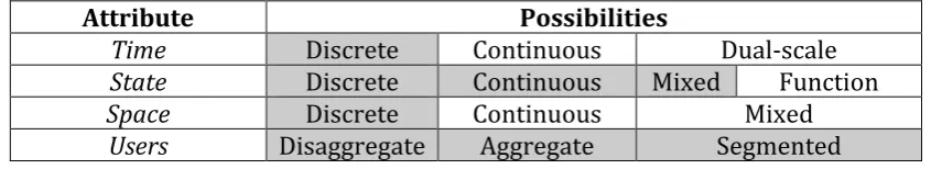
for the theoretical properties that may be established for the model, among other things. Table 1 specifies the elementary components that we shall and shall not permit in the present paper. In the remainder of this section we shall explain in detail the meaning of each of these attributes.
Attribute Possibilities
Time Discrete Continuous Dual-scale
State Discrete Continuous Mixed Function
Space Discrete Continuous Mixed
Users Disaggregate Aggregate Segmented
Table 1: Possible representation of basic elements (shaded cells are the possibilities permitted within the theoretical framework of the present paper)
2.1 Representation of time
Perhaps the most fundamental decision to be made in representing transportation system dynamics is how to represent time. In order to understand this issue we need first to define the application context of the class of modelling problems we shall consider, namely to problems of transport planning over some given future planning horizon of weeks or years (though often it may not be explicitly defined). This application domain distinguishes them in particular from operational models that be used for optimizing short-term system performance over a periods of a few minutes or hours. Within this context, a central element of the models we shall consider will be the adaptive behaviour of travellers over time, as they repeat the requirement to make certain travel decisions. For example, this may be a traveller, or group of travellers, deciding on a residential or work location (a decision perhaps reviewed over periods of years). Alternatively, the traveller may be a commuter choosing a mode and route/service to work each morning, a decision which might be reviewed over days or weeks; even if this choice is stable, the decision to continue with a previous choice is then also being made, at least in our models if not consciously by travellers. In the latter (commuting) example day-to-day dynamics has been suggested as a term to capture this idea of repeated decision-making and adaptation.
Therefore, we shall argue, time in some sense naturally divides into discrete epochs of time (be they individual days, weeks or years) over which travellers review their travel decisions. Cascetta (1989) when introducing the notion of an epoch in this context noted:
‘... epochs can have either a “chronological” interpretation as successive reference periods of similar characteristics (e.g. the a.m. peak period of successive working days) or they can be defined as “fictitious” moments in which users acquire awareness of path attributes and make their choices’.
[image:5.595.86.514.140.217.2]called the ‘within-day scale’ (or, more generally, the ‘within-epoch scale’), in contrast with the comments above on the ‘between-day’ or ‘between-epoch’ scale.
Thus, unless we do truly model 24 hours of each day, our argument will be that it is natural to restrict attention to models in which the between-epoch scale is discrete, and for this reason we only consider such processes in the present paper. This is not a necessary restriction, and indeed there exist counterpart results for continuous-time stochastic processes that we could have considered (see: Fan & Liu, 2007; Hofbauer & Sandholm, 2007). The within-epoch scale is somewhat different, and in this case we might argue either for a discrete- or continuous-time representation, but to simplify the exposition, we suppose the within-epoch time-scale is also discrete. Again, this is not necessary, and we could in principle specify stochastic processes with a ‘dual-scale’ of mixed discrete/continuous for between/within-epoch time respectively, but we would pay significantly in terms of mathematical complexity in that the random state variables we introduce in section 2.2 below would all then be random functions of time.
2.2 Representation of state & distributions
Having restricted attention to discrete time processes, as explained in section 2.1, we move on to the second element of Table 1, namely the definition of state, and at this stage we can begin to introduce some notation. We denote the discrete time epochs ( between
-epoch time or day-to-day time by the letter t (for t = 0, 1, 2,...), the state vector describing epoch t as x(t), and the state-space to which any state must belong as a set , i.e.
x(t) (for t = 0, 1, 2,...). This compound state vector may contain several different kinds of
entitysuch as choices and memories of travellers, and experiences of travel timesmeasured at some chosen level of aggregation, and describing within-epoch
within-day time variations in time and space. The details are important, and we shall delve into them in the remainder of the paper, but for the moment the key issue is that x(t)
is a sufficient description in two respects:
A1 if we know x(t) then we know (or can infer) everything we might want to know from
the model for the purposes of design or evaluation; and
A2 if we know x(t) then we have sufficient information to write down a probability law
that determines the probabilities of all future states of the modelled transportation system for times t +1, t + 2, ....
Assumption A1 implies that model outputs are sufficient for the intended purpose, both in terms of what they measure and their level of aggregation, but does not preclude the subsequent application of sub-models to infer further outputs; for example, it may be that x(t) itself does not contain a pollution level variable, but contains information on
explanatory variables (flows, speeds, etc.) that might subsequently be fed into a pollution sub-model for evaluation purposes. On the other hand, assumption A2 implies that if the future evolution of the transport system were somehow dependent on the pollution levels (e.g. affecting the choice of residential location), then they would need to be in x(t).
of x(t) to be the history h(t) (x(t 1), x(t 2), ..., x(0)) in order to preserve the Markov
property, since then our state space is either finite-dimensional but evolving as the size of h(t) (and hence x(t)) expands with time t, or is infinite-dimensional in order to incorporate a priori all histories of any dimension (including as t). We shall see that aside from the standard device of requiring any such histories to have a fixed, finite length, we can also (by appropriate choice of state variables) also incorporate what are apparently infinite histories by a judicious choice of state variable. We return to illustrate this with examples in section 3, but for the moment our purpose is simply to highlight the key nature of Assumptions A1 and A2, and the care needed in ensuring that they are satisfied.
A quite separate issue is what kinds of variables might be in the space . We shall assume that either is finite and formed from integer n-tuples (i.e. n), or that is part of m -dimensional Euclidean space ( m), or that is a combination of these two kinds of variable (i.e. = 1 2 n m). Thus we permit discrete, continuous and mixed
discrete/continuous state-spaces; we provide examples of each of these later, in section 3.
The assumptions made thus far allow us to introduce some basic, general notation to describe the evolution of the stochastic system. In order to allow different kinds of (discrete, continuous or mixed) state-space, we adopt a particular form of notation that might apply to either case. In particular:
at any given time epoch t, let {q(t)(x) : x } denote the (epoch t) joint probability/
probability-density function across the possible states x (for t = 0, 1, 2...) (we
shall refer to this as the state probability distribution at time t ; and
for any given state y and given parameter vector , let {(x, y; ) : x } denote the conditional joint probability mass/density function across possible states x in the current time epoch, given that y was the state in the previous
time epoch we shall refer to this as the transition function
It should be noted that we assume the transition function to be time-independent, and
the parameter vector to be fixed and time-independent. Together, these imply that
the resulting process is time-homogeneous. The assumptions above imply that the joint probability/ probability-density function of x varies in time only due to one factor, namely due to the state y in the previous time epoch. While this assumption may seem somewhat restrictive, we shall illustrate in section 3 how it can accommodate just about any form of model that has been proposed to date in the transportation literature, and provides a framework for many more not yet proposed. As we show in section 3 (e.g. example 3.2), we can easily accommodate a dependence on a finite number of past states (i.e. not just yesterday by making a component of the state variable a finite history up to that day and by judicious choice of state variables can even in some cases include apparently infinite histories (e.g. section 3.3).
the same decisions/recommendations regardless of the current clock-time t. This is true even for so-called anticipatory systems since even they cannot know the future, they too must be driven by forecasts of or plans for the future, based on historic information. For the interested reader, examples of a stochastic process model in interaction with some responsive control systems (signal control and demand-responsive bus operations) are discussed in Watling (1996).
Based on the assumptions made to date, we may then write our stochastic process as one of the following1, depending on the nature of the state-space:
For any given initial distribution {q(0)(x) : x }, then for t = 1, 2, ...:
i) Markov Process:
q(t)(x) = y (x, y; ) q(t 1 )(y) dy (x m; )
ii) Markov Chain2:
q(t)(x) = y (x, y; ) q(t 1 )(y) (x n; )
iii) Markov Process/Chain
q(t)(x) q(t)((x[1],x[2])) =
y[1] [1] y[2] [2] ((x[1],x[2]),(y[1],y[2]); ) q(t 1 )((y[1],y[2])) dy[2]
(x (x[1],x[2]), x[1] [1] n; x[2] [2] m; ).
All cases require a distribution {q(0)(x) : x } to initialise the process, and this may arise
from one of several sources. One possibility is that it has been estimated by observation of
some current conditions (if t is the present . In this way, it acts more like an additional set of parameters, and indeed we may even choose to parameterise the initial distribution itself, with the task then to estimate the parameters of the initial distribution from observation. A second possibility with discrete state-space is to specify {q(0)(x) : x
} by setting all probability at a single point in the state-space; the justification might be
that the past is certain the future is uncertain. A third possibility is that {q(0)(x) : x } is
generated by the end-point of an earlier application of the stochastic process approach (where end-point may mean the distribution at some given time t = T or an infinite-time stationary distribution). This idea of using an earlier application sits particularly well with the idea of a before-and-after study of some hypothetical scheme, for example, whereby the process is first used to replicate the time prior to the implementation of the scheme, and the resulting distribution then used to initialise a model of the situation after the scheme implementation.
Aside from the initial distribution, the three specifications given also have the common feature that each includes the functions and q, and in each specification these functions perform the same role: in simple terms we might say that is the model and for time t = 1, 2, ...) then qis the unknown as we now explain The function is parameterised by the
1 Note that we could combine these cases as a single case by use of a Riemann-Stieltjes integral.
2 If our interest had only been in models with a discrete, finite state space, then a simpler, standard
specification would be as q(t) = Pq(t 1), with the states in labelled 1, 2, ..., | |, the transition probabilities in a
vector which we assume to be constant3, and something that the modeller specifies at the
start of the process; it is a collection of all parameters across all sub-models. (x, y; ) also depends on the vector y yesterday s state and whenever we apply in the formulae above, we do so in a recursive way in which y is effectively known as we consider all the possible yesterday states in . In this way, y also acts as a kind of parameter, although we do not assign it a particular value but consider all its values across . (x, y; ) may then effectively be thought of as a function of x only, given knowledge of y and , a function that expresses the spread of likely values of x for today when we are given that y occurred
yesterday and assuming that the model parameters are given in ). In order to specify this spread of likely values (formally, conditional probabilities), we shall typically specify a series of sub-models, so that the function is a rather complex, composite function that arises from the combination of these sub-models. Typically we will not want or need to actually write down but will instead specify it by implication, by setting out a series of conditional statistical assumptions for the model components, as we shall see in the examples in section 3.
In this way, like the initial distribution {q(0)(x) : x }, the function is also something
that is assumed to be known and specified by the modeller, before application of the equations above. What the equations above allow is for {q(0)(x) : x } to be combined
with to produce {q(1)(x) : x }, and then for {q(1)(x) : x } to be combined with (the
same function) to produce {q(2)(x) : x }, and so on. Thus the objective of the modelling
process can be viewed to be that of recursively generating a sequence of probability distributions {{q(t)(x) : x } : t = 1, 2, ... }, given knowledge of {q(0)(x) : x } and . This
sequence of probability distributions is the model output in theory at least although in
practice we may find it sufficient to only store/record some summary measures of the distribution, or indeed (in a spirit similar to equilibrium analysis) may not refer to the temporal evolution at all an issue to which we shall return later (see section 4.2).
2.3 Representation of space
Given the possibilities presented in sections 2.1. and 2.2 for how to represent time and state, the modeller then has several choices for how to represent the detailed elements of the transportation system, within the framework of possibilities given by section 2.1/2.2. In Table 1, we have suggested that the third such element is the question of how to represent space. To be clear, we are not intending to suggest that the question of spatial representation is something unique to adopting a stochastic process approach, rather the particular issue faced is deciding on the type of representation in conjunction an appropriate state representation, since this may have profound effects on the theoretical properties that may be established for the chosen model.
Discrete space models are undoubtedly the most proliferous in the transportation literature. In public and private transport models, the dominant representation of the
3 At this stage this is not a necessary assumption, and in fact we may wish to consider models in which
physical infrastructure is through a discrete graph. On the other hand, diachronic networks may be used to represent feasible temporal connections, especially in the case of public transport services (Wilson & Nuzzolo, 2009). A different spatial question is how vehicles move within the infrastructure. For ease of implementation we may choose to approximate the dynamic movements in continuous space along the arcs of a discrete spatial graph, by adopting a further discretisation scheme as in the cellular automaton (Rickert et al, 1996) or cell transmission (Daganzo, 1994) approaches. In spite of the dominance of discrete-graphs, alternatives based on a continuous representation of space have existed for many years (e.g. Dafermos, 1980), and may be justified as an approximation to discrete infrastructure needing less parameters or less data. For cases such as pedestrian route choices the available space within which routes are chosen is ontologically continuous (and so there is no obvious discrete graph with which to begin), meaning that a continuum model is an obvious option to consider (Wong, 1998; Hoogendoorn & Bovy, 2004; Huang et al, 2009). For many land-use/transport interaction problems a continuum representation is also rather natural, for example given the continuous nature of new residential locations (Ho & Wong, 2007). A third possibility is a
mixed spatial representation, such as one in which a continuum representation of demand is combined with a discrete graph of the infrastructure, or where different levels of detail are appropriate for different parts of a street network (Guo & Liu, 2012). A particularly familiar, mixed spatial approach is one in which vehicles are moved continuously in space (though discretely in time) along a discrete street network, as in car-following-type micro-simulation models (see the example of section 3.6).
2.4 Representation of users
Completing our consideration of Table 1, the final issue of representation is concerned with the users of the transportation system. In a similar way to the treatment of space, at least some of the issues in representing users are familiar ones faced in all transportation modelling exercises, and in such cases the key point is again to be aware that the choice of representation may imbue the process with particular theoretical properties. However, the representation of users differs to that of spatial representation in that there are special modelling considerations that only arise because we are adopting a dynamic process approach (be it deterministic or stochastic). So the purpose of the present section is also to indicate these special considerations, and the options that are available in those cases.
The most familiar issue to consider in the representation of users is the level of detail at
which we represent a users decisions and b the stimuli that motivate those decisions )n
behaviour and probability is a device for describing the uncertainty of modellers in
explaining individuals behaviour Aside from these conceptual points, we have a possibility commonly used in traditional models of some kind of fixed segmentation of users, applying the models described above within a segment/user-class.
As noted at the outset, there are also special issues that arise in representing users within a dynamic process framework. These concern the dynamics of how users remember and learn from their experiences in order to make predictions (upon which their choices are made), and also the extent to which they display inertia/habit in their propensity to reconsider previous choices. In the present section we are not concerned with the detailed assumptions of these model components (such details will emerge in the remainder of the paper, and the references therein), but rather to indicate that exactly the same issues of aggregation/disaggregation/segmentation arise for these elements as were identified above for the modelling of the decision behaviour. While we might typically expect the same level of aggregation to be chosen for all such elements (experience, learning, habit, choice), there may be also be cases in which different levels of aggregation are appropriate. For example, in modelling the longer-term impacts of driver information systems, we might models users making choices and gaining personal travel experiences at the individual level, but part of the effect of the information system might be represented by pooling the experiences of all users after journeys have been completed.
3. MOTIVATING ILLUSTRATIVE EXAMPLES
Having introduced a rather general framework for stochastic process modelling in a transportation systems context, it is now possible to move on to specifying particular families within this framework in section 5, but before moving on to these general families, we provide in the present section some deliberately simple examples. We will derive explicit transition functions (as defined in section 2.2) for particular models. While it would be possible to implement the models without explicit derivation of the transition function (e.g. through Monte Carlo simulation), we wish to highlight here the theoretical equations behind the model rather than its implementation. As we shall see in later sections, understanding the transition function is the key to establishing overall theoretical properties of the modelling approach. A further objective is to demonstrate the generality of the stochastic process approach in its possibility to link to fields such as dynamic traffic assignment and micro-simulation; it should not be considered as a particular model, but rather a way of modelling which encompasses many particular models and approaches.
3.1 Example 1: Myopic learning with discrete state space
Cascetta (1989) introduced a family of discrete state space stochastic process models to the transportation field. The simplest example within this family is that of a network consisting of two parallel arcs/routes serving a given integer OD demand d, such that we may represent the state of the network by an integer scalarx denoting the flow on arc 1 (with the flow on arc 2 then clearly d x). Thus, in this example our state space is given by = {0, 1, 2, ... , d}, and we are appealing to specification ii) in section 2.2, that of a Markov Chain. Let ci(; ) be the performance function on arc i (i = 1,2), parameterised in total by the vector , with the performance function denoting the cost to traverse the arc as a function of the flow on that arc only4. Thus, given state x, the arc costs are c
1(x; ) and
c2(d x; ), and for ease of notation it will be convenient to define a scalar function for the difference in actual arc costs:
c(x; ,d) c1(x; ) c2(d x; ) .
Suppose that drivers as a group remember only the costs experienced (as a group) on the previous day. Then, on any given day, conditionally on the remembered costs, each of the d
drivers is supposed to choose between the routes independently and at random according to a logit choice probability (with scale parameter > 0) evaluated at the remembered costs. The parameters of the overall model may be collected together in the vector
= (, d, ). The assumptions together imply that the transition functioni.e. the conditional probability distribution of the flow x on arc 1 on any one day, given that the flow on arc 1 was y yesterdayis given by the Binomial expression:
(x, y; ) = {d!/(x! (d x)!)} . {1/{1 + exp(c(y; ,d))}}x . {1 {1/{1 + exp(c(y; ,d))}}}d x (for x = 0,1,...,d; y = 0,1,...,d; = (, d, )). with the expression above we have all that is needed to generate the state probability distributions for times t = 1, 2, ..., given an initial t = 0 state distribution. Denoting the initial state probability distribution is {q(0)(x) : x = 0, 1, 2, ... d}, then the state probability
distribution at time t = 1 is (applying the Markov Chain expression in section 2.1):
q(1)(x) = y {0,1,2,...,d}(x, y; ) q(0)(y) (x = 0, 1, 2, ..., d) .
That is to say, it is a mixture distribution of Binomial variables with mixture probabilities given by the initial state distribution. Given q(1)(x), we may then compute q(2)(x) by the
same process, and so on.
3.2 Example 2: Learning processes and retaining the Markov assumption
While Example 1 may be extended in many ways, a basic limitation it has is the assumption
that drivers remember only the previous day s travel costs which was later termed myopic behaviour From early evidence the assumptions regarding how drivers learn
was known to be both (a) highly influential on the plausibility of predictions of the overall model (e.g. Horowitz, 1984) and (b) something for which there was evidence of non-myopic behaviour (e.g. Chang & Mahmassani, 1988; Iida et al, 1992). The simplest extension of Example 1 within the discrete-state framework proposed by Cascetta (1989) is to assume that drivers now remember some finite number of previous days costs, and form their predictions of costs for the forthcoming day based on a weighted moving average. As a simple example, suppose that drivers remember only costs on the previous
two days weighting yesterday s costs by and the costs from two days ago by 1 , for given 0 < 1. Our state variable now is extended to be a two-dimensional vector x with x1 and x2 respectively denoting the flow on arc 1 that occurred today and yesterday. Thus,
now our state space 2 is given by = {(x1,x2) : xi {0, 1, 2, ... , d} for i =1,2}, and again
we are able to appeal to (the Markov Chain) specification ii) in section 2.2. Retaining all other assumptions made in Example 1, the parameters of the overall model may now be collected together in a slightly extended vector = (, d, , ).
Now we aim to write down the transition function. For example, we must describe how a pair of states on days 1 and 2 transforms into a pair of states on days 2 and 3. Now, given knowledge of the states on days 1 and 2, then there is no uncertainty regarding the state on day 2, and so the only pairs of days 2/3 states with non-zero conditional probability of being transformed into are those that have the same given state on day 2. Now in general in the notation given, the sequence of consecutive states that interest us (i.e. give non-zero conditional probability) are over a period of 3 consecutive days: y2, y1 = x2, x1
(corresponding respectively to the day before yesterday, yesterday and today). The conditional probability that the states (today, yesterday) are (x1, x2) given that the states (yesterday, day-before-yesterday) were (y1, y2) is therefore zero if x2 y1 , and is otherwise
equal to the conditional probability that today s state is x1 given that the states (yesterday, day-before-yesterday) were (y1, y2). Overall, this implies that the transition function, while now a function of vector states,turns out to be a quite simple modification of that given in Example 1, namely the combination of a Binomial expression and an indicator function:
(x, y; ) = {d!/(x1! (d x1)!)} . {1/{1 + exp(( c(y1; ,d) + (1 )c(y2; ,d)))}}x1 .
{1 {1/{1 + (( c(y1; ,d) + (1 )c(y2; ,d)))}}}d x1( x2 , y1)
(for x ; y ; = (, d, ,))
where (a,b) is the Kronecker delta function:
(a,b) = 1 if a = b
= 0 if a b .
As well as having a difference from Example 1 in the manner that state transitions are defined (in that we must consider pairs of states), there is also a difference in the state distribution, which likewise pertains to pairs of states on consecutive days. So our initial state probability distribution at time t = 0 is now actually a specification of the joint probability distribution of the arc 1 flow at time t = 1 and time t = 0.
A point often misunderstood is that this truly is a joint distribution, and so we may have correlations between the same variable on consecutive days (so-called auto-correlations). These auto-correlations persist and evolve as the process evolves, just as the marginal probability distributions evolve of the flows on any one day; looking ahead to section 3, they persist even when the process is stationary (an issue we shall discuss later).
The initial state distribution5 is thus now denoted {q(0)(x) : x = {(x1,x2) : xi {0, 1, 2, ... , d} for i =1,2}}, each element giving the joint probability that the day 0 arc 1 flow is x1 and the day 1 arc 1 flow is x2. However the initial joint state distribution is generated, the
5 In practice, we may wish to simplify the specification by using a model of the form given in Example 1 to
state distribution on day 1 (a bivariate distribution of the flows on days 1 and 0) is generated according to:
q(1)(x) = y (x, y; ) q(0 )(y) (x )
and so on for the state distributions on days 2 and beyond.
3.3 Example 3: Exponentially-weighted learning with continuous state space
While the formulation in Example 2 can be extended in the obvious way to weighted moving average learning processes of any finite order, or indeed many other forms of learning process that need not be based on averages, ultimately there has to be a finite limit specified on the number of days of remembered experiences. This is in order that the process has a fixed state-space and retains the Markov assumption, which (as we shall see later) becomes a key element in establishing important theoretical properties. A negative aspect to moving average processes of high order, however, is that they are relatively computationally expensive to implement, since one must retain and update a moving window of experiences. In this respect, an exponentially-weighted process is much more attractive, but if analysed within the framework of Cascetta (1989) it yields a problem of infinite memory. This is a particular case in which being able to adopt different forms of state-space becomes especially convenient. The simplest example of this arises from an instance from the family considered by Cantarella & Cascetta (1995), a model used for analysing a deterministic dynamical system by Watling (1999). We consider the same example as Example 1, except that now we suppose that drivers using an updating process for their predicted costs for their forthcoming journey. Indeed these predicted costs become so central that we define a scalar state variable x now to be the difference in predicted cost given by the predicted cost on arc 1 minus the predicted cost on arc 2, with our state space now = Given that yesterday s predicted cost difference was y, and given that yesterday s actual cost difference was z then we suppose that today s predicted
cost difference x would simply be a weighted average of these two, x = z + (1 )y for some parameter typically assumed to satisfy 0 < 1. (It is noted in passing that the special case = 1 corresponds to the simple model considered in Example 1.)
Now, given that yesterday s predicted cost difference was y, then according to the assumption that drivers choose independently and at random according to logit choice probabilities based on the predicted costs, we know the probability distribution of
yesterday s flow on arc 1:
Pr yesterday s arc flow f yesterday s predicted costs were y) =
{d!/(f ! (d f)!)} . {1/{1 + exp(y)}}f . {1 {1/{1 + exp(y)}}}d f (for f = 0,1,...,d; y ).
and so this also gives a distribution of the actual cost differences conditional on y: Pr yesterday s actual cost difference c f) yesterday s predicted costs were y) =
be achieved, but the most convenient to illustrate in the present context is one in which we begin by making the flow variables continuous.
In particular, we assume that d is sufficiently large and that the probability of choosing any arc is sufficiently far from 0 or 1, that we may use the Normal approximation to the Binomial distribution, so that if F and Y denote the random variables corresponding to f
and y, then:
F | Y = y ~ Normal( d/{1 + exp(y)}, {d/{1 + exp(y)}}{1 {1/{1 + exp(y)}} ) . For the sake of this simple example, let us also suppose that the travel cost functions are affine, leading to an actual cost difference function of:
c(f; ,d) c1(f; ) c2(d f; ) = (1 + 2 f ) (3 + 4(d f )) = (1 3 4d) + (2 + 4) f .
Thus as an affine transformation of a Normal random variable yesterday s actual cost difference conditional on yesterday s predicted cost difference is also Normal using Z to denote the random variable corresponding to z as introduced earlier):
Z | Y = y ~ Normal( (1 3 4d) + d(2 + 4)/{1 + exp(y)},
{d(2 + 4)2/{1 + exp(y)}}{1 {1/{1 + exp(y)}} ) .
)t follows finally that today s predicted cost difference X = Z + (1 )Y, when conditioned on Y = y, is also Normal:
X | Y = y ~ Normal({(1 3 4d) + d(2 + 4)/{1 + exp(y)}} + (1 )y , {d2(2 + 4)2/{1 + exp(y)}}{1 {1/{1 + exp(y)}} )
and so our transition function can finally be defined in the Markov Process form i) from section 2.2, as the Normal density:
(x, y; ) = (2{d2(2 + 4)2/{1 + exp(y)}}{1 {1/{1 + exp(y)}}) 0.5
exp( 0.5{x {{(1 3 4d) + d(2 + 4)/{1 + exp(y)}} + (1 )y}2/
{d2(2 + 4)2/{1 + exp(y)}}{1 {1/{1 + exp(y)}} )
(for < x < ; < y < ; = (, d, , )) .
Thus we have managed to retain the Markov property with a complete representation of the stochastic process over , in contrast with Examples 1, 2 which were defined over
The state distributions {q(t)(x) : < x < } generated by this process, as well as the initial
state distribution at t = 0, are then clearly probability density functions as opposed to probability mass functions as they were in Examples 1 and 2. Note also that in the special case = 1 we obtain a continuous approximation to the discrete model presented in Example 1.
3.4 Example 4: Modelling user habit with a mixed state space
The examples above provide illustrations of the usefulness of state space representations in n and n; in the following example, we illustrate the usefulness of the final, mixed
representation iii) specified in section 2.2, again referring to a simple example from the family proposed by Cantarella & Cascetta (1995). In particular, starting from the two-route
example so far considered we now introduce the notion of habit, given the quite strong
reconsider their previous day s choice and make choices according to a logit model, as in earlier examples, with a -type learning model (as used in Example 3) used to update the predicted travel costs. With probability 1 travellers choose between the available routes with probabilities equal to the fraction of travellers that actually chose each of those routes on the previous day. Unlike Example 3, we shall retain the discrete nature of the flow variables (and so not make a Normal approximation to the Binomial). However, we will face a similar difficulty effectively in how to generate continuously-distributed actual costs from discrete flows, but here we shall adopt a different strategy of assuming:
a) the travel cost functions provide a mean for a given level of flows, and that the actual cost for a particular day, given the flows for that day, is distributed according to a continuous random variable about that mean; and
b) the predicted travel cost for the forthcoming day also has a random residual term associated with it, with mean equal to the learning filter based on the actual costs above.
As an example of assumption a), we specifically assume stationary Multivariate Normal random errors for the actual arc costs, and this will imply a univariate Normal random
error in the actual cost difference between the two arcs/routeslet us suppose that this
resulting, univariate Normal random error has mean 0 and variance 2. By a similar logic,
in view of assumption b) we shall assume that the predicted travel cost is distributed about the learning filter according to a stationary Normal distribution with mean 0 and variance 2. We note that exactly the same strategy of introducing these error terms could
have been adopted in Example 3, avoiding the need for the Normal approximation; the only reason to adopt the Normal approximation and affine cost functions in that case was in order to choose an example that allowed us to illustrate an analytic form for the transition function. (It is noted in passing that in the degenerate case = = 0, the
corresponding normal density functions appearing in the transition function below are replaced by Kronecker delta functions.)
In the present example, we shall adopt a three-dimensional, mixed discrete/continuous state variable x = (x1, x2, x3), where x1 {0, 1, 2, ... , d} is the flow on route 1, x2 is the predicted cost difference (at the beginning of the day) and x3 is the actual cost difference experienced (on that day). Now our aim will be to write down the joint conditional probability mass/density function of the random variable X = (X1, X2, X3), given
that yesterday s state was Y = y = (y1, y2, y3), It is first worth noting that there is conditional dependence between the component variables in X given Y, and therefore we cannot simply hope that the joint distribution of X | Y is the product of the marginal distributions of X1 | Y, X2 | Y and X3 | Y. On the other hand, we can see there is logical sequence
(dependence structure) in considering the components of X. This can be seen since X2 | Y
depends only on Y (and not additionally on X1 | Y and X3 | Y), X1 | Y depends only on Y and
X2 | Y (not additionally on X3 | Y), and X3 | Y depends only on X1 | Y (not additionally on X2 |
Y). Therefore we may instead write with by a slight abuse of notation Pr denoting probability density or probability mass function as appropriate):
Pr((X1, X2, X3)| Y) = Pr(X2 | Y) . Pr(X1 | Y, X2) . Pr(X3 | Y, X1) .
We may determine each of the component distributions in this product. Considering firstly X2 | Y = (y1, y2, y3), then this distribution has two influences. On the one hand, its mean is
E[X2 | Y = (y1, y2, y3)] = (1 ) y2 + y3 .
The second influence is the assumed error distribution of the predicted cost about this mean, yielding:
X2 | Y = (y1, y2, y3) ~ Normal((1 ) y2 + y3 , 2).
Now we move on to consider the distribution of X1 | Y = (y1, y2, y3), X2 = x2 . With the
extended behavioural model, travellers now are assumed to have two reasons for choosing
route 1 (over route 2): either they choose it out of habit based on a probability of y1/d (the fraction of drivers that actually chose that route yesterday), or they choose it according to
a logit model based on today s predicted cost differencex2. The probability of choosing for the first reason is 1 and for the second reason is . This combination of assumptions
implies:
X1 | Y = (y1, y2, y3), X2 = x2 ~ Binomial( d , {(1 ) y1/d} + /{1 + exp(x2)} ) .
Finally we consider the distribution of X3 | Y = (y1, y2, y3), X1 = x1 . In an analogous way to
the predicted cost difference, the distribution of the actual cost difference was two influences: its mean is determined by the link performance functions and its variation about the mean by a stationary Normal random error term. Assuming as in Example 1 that the mean arc cost difference is given by a difference in performance functions denoted by c(; ,d), then we have:
X3 | Y = (y1, y2, y3), X1 = x1 ~ Normal(c(x1; ,d), 2) .
Thus we are in a position to construct the complete transition function (i.e. the complete conditional joint probability density/mass function) as a product of the three component distributions derived above:
(x, y; ) = {d!/(x1! (d x1)!)} . {{(1 ) y1/d} + /{1 + exp(x2)}}x1 .
{1 {(1 ) y1/d} /{1 + exp(x2)}}d x1 .
(2) 0.5 exp( 0.5((x2 (1 ) y2 y3)/)2 ) .
(2) 0.5 exp( 0.5((x3 c(x1; ,d))/)2 )
(for x1 = 0,1,...,d; < x2 < ; < x3 < ; y1 = 0,1,...,d;
< y2 < ; < y3 < ; = (, d, , , , , ) ). To derive the state distributions we now must use formulation iii) in section 2.2, in which the state space is split into a discrete and continuous component in this case, the discrete component corresponding to x1 and the continuous component to (x2, x3). Thus, the state
distributions that arise for t = 1,2, ..., {q(t)(x) : x1{0,1,2, ...,d}; < x2 < ; < x3 < }, as
well as the initial t = 0 distribution, have both a discrete and continuous component. In order to facilitate the specification of the initial joint distribution, a decomposition strategy analogous to that carried out above should be performed.
3.5 Example 5: Dynamic traffic assignment in a stochastic process context
based on a discretisation of the origin time-period modelled within each day into n
departure periods, for some given n. Assuming first-in-first-out to hold, then a travel time may be imputed for each departure period, by comparison of the cumulative in-flows to each link with the cumulative out-flows from that link. Let us suppose that the origin-destination demand flow in each departure period i is given by the constant integer di for i = 1,2,...,n, and let xi denote the flow that choose to use route 1 when departing in time period i, for i = 1,2,...,n. Let x = (x1, x2, ..., xn) thus be the state vector, with state space:
= {(x1,x2, ..., xn) : xi {0, 1, 2, ... , di} for i =1,2, ..., n} .
For any given x the flow profile entering route 2 is d x , and so given x we may apply the CTM as described above to obtain a unique travel time for each route for each entry period (forming a weighted average across the entry period when traffic exits in different exit time periods). For each entry period, suppose that we record the travel time on route 1 minus the travel time on route 2. The relationship between x and these travel time differences may therefore be represented as a vector function c(x ; ,d), where c: n
and where denotes the vector of parameters of the CTM across both links.
Assuming that as in Example drivers consider only the previous day s travel time
relevant to the departure period in which they are travelling, that for simplicity we simply assume all parameters hold for all time periods, and that conditionally on the past drivers choose independently between time periods, then the transition function for this model is a simple extension of that presented in Example 1:
(x, y; ) = i{1,2,...,n} {di!/(xi! (di xi)!)} . {1/{1 + exp(ci(y; ,d))}}xi .
{1 {1/{1 + exp(ci(y; ,d))}}}di xi (for x, y ; = (, d, )).
The fact that such an apparently simple model arises is due to the conditional independence assumption, yet this is not such a strong assumption; effectively it means that while drivers travelling at the same time and at different times of day will have had commonalities and correlations in their past experiences, that once this experience is gained they do not then collude in making decisions on any particular day (analogous to
the selfish routing principle behind the Wardrop equilibrium concept Certainly travel times do not separate by time-of-departure (note that ci above depends on the vector y). Indeed when this transition function is used within the Markov chain model ii) in section 2.2, the resulting state distributions {q(t)(x) : x }will in general be joint distributions
that are correlated across departure time periods, and for more general learning models auto-correlated over between-day time (see Balijepalli et al, 2007). We remark that the same approach could be used for extending examples 2, 3 and 4 given earlier.
3.6 Example 6: A theoretical basis to micro-simulation
The examples considered so far all assumed drivers to act as an aggregate, but we may also disaggregate drivers to any desired level. At an extreme, we may model individual drivers with their own individual-specific attributes, thus providing a theoretical basis for the computational method known as (discrete) micro-simulation. For illustration, we shall adapt Example 4 (simplifying to no habitual effect, i.e. = 1 in the notation of Example 4) to follow the spirit of a model presented in Liu et al (2006). We shall suppose three inter-related aspects to the micro-simulation: in the propagation of individual vehicles through the network along given routes, in the way in which individuals learn from their own (but
Let f = (f1, f2, ..., fd) be a vector of 0/1 indicator variables, with fi = 1 only if individual i selects route 1 (rather than route 2) for i = 1,2,...,d. Suppose that each individual possesses a vector of individual-specific, traffic-related behavioural parameters which determine
factors such as that individual s preferred departure time their aggressiveness in
accepting gaps when car-following or lane-changing, and the performance characteristics of the vehicle they drive. Suppose that all such parameters are collected together across all individuals in a single parameter vector . All of these factors account for drivers having a systematically individual-specific experience of travel time on the route that they choose to follow. Let ci(f; ) denote the mean travel time individual i would experience on their chosen route (i.e. on route 1 if fi = 1 in the argument f or on route 2 otherwise), when the population of drivers choose routes according to f and when the population has individual traffic-related behavioural parameters given by . Suppose that the actual travel time experienced by each individual i is a random variable given by ci(f; ) + i (for i = 1,2,...,d), where (1, 2, ..., d) are independent and identically distributed Normal random variables with mean 0 and variance 2. (In realistic micro-simulation models the randomness would
have a more complex source, but we adopt these simplistic assumptions here purely so we can write down an analytic expression for illustration.)
Now an important distinction from the aggregate models considered earlier is that when drivers learn, they learn only of the travel time on the route they actually chose, whereas for the unchosen alternative they leave their prediction of travel time unchanged (presumably in the real world an intermediate behaviour occurs). The fact that individuals learn individually means that we cannot utilise the strategy used in the aggregate examples, whereby only the difference in travel time between the routes is updated, but instead must separately record/update the predicted travel time for each route, for each individual. We shall use a weighted average learning model for the chosen route, as was used in Example 4, but here applied to each individual. This learning model provides the mean predicted cost for each route for each individual i, and to this we add a zero mean, Normally distributed and individual-specific error term, that is independent and identically distributed across individuals with variance k2 for route k = 1,2. Based on
these predicted costs, each driver chooses a route based on a logit model with common scale parameter .
In order to represent this model we shall use a state variable x = ({0,1} 3)d which contains four items of information for each individual, stacked in order of individual number. Thus individual is variables are the elements x4i 3 , x4i 2 , x4i 1 and x4i (for i = 1,2,...,d) denoting:
x4i 3 = 1 if individual i chose route 1, and = 0 if route 2 chosen x4i 2 = individual is actual travel time on their chosen alternative x4i 1 = individual is predicted travel time on route
x4i = individual is predicted travel time on route
Conditional on yesterday s state y, then we can first compute the new mean predicted
travel times on each route. We do this by first noting that we may use y4i 3 and 1 y4i 3for routes 1 and 2 respectively as a form of indicator variable, each equal to 1 only if that route was the chosen route, and equal to 0 otherwise. Thus our learning model only updates the route that was chosen. For each individual i = 1,2,...,d we then have:
x4i = y4i + (1 y4i 3)( y4i 2 y4i) .
Thus, when we consider the predicted travel times as random variables (by adding the iid error terms to the mean predicted travel times above) we obtain the two sets of conditionally independent distributions:
X4i 1| Y= y ~ Normal(y4i 1 + y4i 3 ( y4i 2 y4i 1) , 12) independently for i = 1,2,...,d
X4i| Y= y ~ Normal(y4i + (1 y4i 3) ( y4i 2 y4i) , 22) independently for i = 1,2,...,d.
Given these predicted costs each driver s choice of route for the present day is a Bernoulli
trial, for each individual i = 1,2,...,d independently:
X4i 3 | X4i 1 = x4i 1, X4i = x4i , Y = y ~ Bernoulli(1/{1 + exp((x4i 1 x4i))}) .
Finally, based on the choices made by all individuals, the actual cost for each individual on their chosen route is the sum of an individual-specific systematic component, and an individual-specific iid random error, such that for each i = 1,2,...,d independently:
X4i 2 | {X4i 1 = x4i 1,X4i = x4i , X4i 3 = x4i 3 , Y = y} ~ Normal(ci(x4i 3 ; ), 2).
Collected together our joint conditional probability mass/density function leads us to an overall transition function of:
(x, y; ) = i{1,2,...,d} {1/{1 + exp((x4i 1 x4i))}}x4i 3 .
(21) 0.5 exp( 0.5((x4i 1 y4i 1 y4i 3 ( y4i 2 y4i 1))/1)2 ) .
(22) 0.5 exp( 0.5((x4i y4i (1 y4i 3)( y4i 2 y4i))/2)2 ) .
(2) 0.5 exp( 0.5((x4i 2 ci(x4i 3 ; ))/)2 )
(for x, y ; = (, d, , , 1, 2,)) .
As for Example 4 earlier, we have a mixed discrete/continuous state-space, and so we use formulation iii) of section 2.2 to model the state transitions.
3.7Example Incorporation of rule-based approaches
Some micro-simulation models are based on a series of if then logical rules rather than smooth, continuous response functions, and it is interesting to see that these also may be incorporated within the framework proposed. As an example, we examine a behavioural rule that has received some considerable attention in the research literature, namely that of bounded rationality (e.g. Hu & Mahmassani, 1997; Guo & Liu, 2010). As a simple illustration, we shall adapt the model presented in section 3.6.
Specifically we will adapt the learning process presented in section 3.6, by assuming that drivers only update their predicted travel times if their latest experience of travel time is significantly different (in absolute terms) from the travel time they anticipated. This provides the following rule:
If |y4i 1 y4i 2| < then
x4i 1 = y4i 1 x4i = y4i else