Clipping in Neurocontrol by Adaptive Dynamic Programming

City, University of London Institutional Repository

Citation

:

Fairbank, M., Prokhorov, D. and Alonso, E. (2014). Clipping in Neurocontrol by

Adaptive Dynamic Programming. IEEE Transactions on Neural Networks and Learning

Systems, 25(10), pp. 1909-1920. doi: 10.1109/TNNLS.2014.2297991

This is the accepted version of the paper.

This version of the publication may differ from the final published

version.

Permanent repository link:

http://openaccess.city.ac.uk/5181/

Link to published version

:

http://dx.doi.org/10.1109/TNNLS.2014.2297991

Copyright and reuse:

City Research Online aims to make research

outputs of City, University of London available to a wider audience.

Copyright and Moral Rights remain with the author(s) and/or copyright

holders. URLs from City Research Online may be freely distributed and

linked to.

City Research Online:

http://openaccess.city.ac.uk/

[email protected]

Clipping in Neurocontrol by Adaptive Dynamic

Programming

Michael Fairbank,

Student Member, IEEE

, Danil Prokhorov,

Senior Member, IEEE

, and Eduardo Alonso

(Cite asClipping in Neurocontrol by Adaptive Dynamic Programming, IEEE Transactions on Neural Networks and Learning Systems, Volume 25, Issue 10, October 2014, pp. 1909–1920. Copyright the authors and IEEE, http://ieeexplore.ieee.org.)

Abstract—In adaptive dynamic programming, neurocontrol and reinforcement learning, the objective is for an agent to learn to choose actions so as to minimise a total cost function. In this paper we show that when discretized time is used to model the motion of the agent, it can be very important to do “clipping” on the motion of the agent in the final time step of the trajectory. By clipping we mean that the final time step of the trajectory is to be truncated such that the agent stops exactly at the first terminal state reached, and no distance further. We demonstrate that when clipping is omitted, learning performance can fail to reach the optimum; and when clipping is done properly, learning performance can improve significantly. The clipping problem we describe affects algorithms which use explicit derivatives of the model functions of the environment to calculate a learning gradient. These include Backpropagation Through Time for Control, and methods based on Dual Heuristic Programming. However the clipping problem does not significantly affect methods based on Heuristic Dynamic Programming, Temporal Differences Learning or Policy-Gradient Learning algorithms.

Index Terms—Clipping, Neurocontrol, Dual Heuristic Pro-gramming (DHP), Backpropagation Through Time (BPTT), Value-Gradient Learning

I. INTRODUCTION

I

time step t, it has state vector ~xt ∈ S. T is a fixed set of

terminal states, withT⊂S. At each timet, the agent chooses

an action ~ut which takes it to the next state according to the

environment’s model function

~

xt+1=f(~xt, ~ut), (1)

thus the agent passes through a trajectory of states

(~x0, ~x1, ~x2, . . .), terminating only when (and if) a terminal

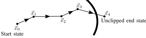
state is reached, as illustrated in Fig. 1. As shown in this figure, clipping is the concept of calculating the exact fraction in the final time step at which a boundary of terminal states is reached, and stopping the agent exactly at this boundary. The name clipping is taken by analogy to the concept in computer graphics. Without clipping, the discretization of time would cause the agent to penetrate slightly beyond the terminal boundary, as shown in the figure.

On transitioning from each state ~xt to the next, the agent

receives an immediate scalar cost Ut from the environment

M. Fairbank and E. Alonso are with the Department of Computer Science, School of Informatics, City University London, London, UK

D. Prokhorov is with Toyota Research Institute NA, Ann Arbor, Michigan Manuscript received June 2013

~ x0

~ x1

~ x2

~ x3

~ x4

Terminal Boundary Start state

Unclipped end state

Fig. 1: A trajectory reaching a terminal state. The thick curved line indicates a boundary of terminal states. In this diagram, clipping does not take place, and the trajectory penetrates beyond the terminal boundary. When clipping is used correctly, we intend to stop the agent exactly at the point of intersection between the trajectory and the terminal boundary.

according to the function

Ut:=U(~xt, ~ut). (2)

In addition, if the agent reaches a terminal state~x∈T, then an

additional terminal cost is given by the scalar functionΦ(~x). Throughout this paper, subscripts on variables will be used to indicate the time step of a trajectory. And from now on in the paper, we will only consider episodic, or finite horizon, environments; that is environments where all trajectories are guaranteed to meet a terminal state eventually.

The ADP problem is for the agent to learn to choose actions so as to minimise the expectation of the total long-term cost received from any given start state ~x0. Specifically, the

problem is to find anaction networkA(~x, ~z), where~z is the parameter vector of a function approximator, which calculates an action

~

ut=A(~xt, ~z) (3)

to take for any given state~xt, such that the expectation of the

following long-term cost is minimised:

J(~x0, ~z) := T−1

X

t=0

γtUt+γTΦ(~xT) (4)

subject to (1), (2) and (3); whereT is the time step at which the first terminal state is reached (which in general will be dependent on ~x0 and ~z), and where γ ∈ [0,1] is a constant

discount factorthat specifies the relative importance of long-term costs over short long-term ones.

The functionJ(~x0, ~z)is called thecost-to-gofunction from

In this paper we show that when a large final impulse of cost Φ(~x) is given at a terminal state ~x ∈ _T, then failure to do clipping in the final time step of the trajectory can very significantly distort the direction of the learning gradient used by certain ADP algorithms, and thus prevent successful solution of the ADP problem. We also show that this problem is not lessened by sampling the time steps of the underlying continuous-time process at a higher rate. This problem affects the commonly used ADP algorithms Dual Heuristic Programming (DHP) [6], [7], and Backpropagation Through Time (BPTT) [8], both of which are described in Section II, plus algorithms based on DHP such as Value-Gradient Learning [9]–[11]. These algorithms are all very closely related to each other [12]–[14], and for purposes of explaining clipping as clearly as possible, we will use BPTT as the example.

BPTT works by calculating the quantity∂J /∂~zdirectly and very efficiently for each trajectory sampled, enabling gradient descent to be performed on J with respect to ~z. However if clipping is omitted then the gradient that BPTT calculates can be distorted enough to prevent learning. Fig. 2 illustrates the problems that arise without clipping.

O t=1 t=2 t=3 t=4 t=5 t=6 t=7

A B

θ d

(a) Spurious zigzag gradients can occur when clipping is not used.

θ R

(b) The graph ofRversusθyields no useful local gradient informa-tion. Hence minimisingRwith re-spect toθusing onlydR/dθwould be impossible.

Fig. 2: An example of the problems that can occur when clipping is not used.

In Fig. 2a the agent starts atOand travels in a straight line at a constant speed, along a fixed chosen initial angle, θ. The straight line AB is a terminal boundary (i.e. a continuous line of states inT). The dotted arcs represent the integer time steps

that the agent passes through. If clipping is not used then the agent will stop on the first integer time step (i.e. on the first dotted arc) after passing the terminal boundary. This means the agent will finally stop at a point somewhere on the bold zigzag path from A to B. In Fig. 2b we see how the distance the agent travelled before stopping (R) varies with θ. If the cost-to-go functionJ was defined to be the total distance travelled before termination (i.e. ifJ:=R), and the parameter vector ofJ was defined to beθ, then the ADP objective would be to minimise

R with respect toθ. But Fig. 2b shows that there is no useful gradient information for learning, since ∂J /∂θ =∂R/∂θ = 0, whenever it exists, and hence gradient descent on J with respect to θ would fail without clipping.

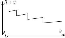
Situations can get even worse than this: In Fig. 3 we show a pathological example where the gradient of the graph is always in the opposite direction of the global minimum of R. This

could occur for example if we were trying to minimise the functionJ :=R+ywith respect toθ, for the situation in Fig. 2a, where y is the final y-coordinate of the agent, and R is the distance travelled before stopping.

θ R+y

Fig. 3: A pathological example: Local gradient is opposite to global gradient.

In general, increasing the sampling rate of the discretization of time will not solve the problem, since that would simply make the dotted arcs in Fig. 2a squeeze closer together, and will make the teeth of the saw-tooth blade shape in Fig. 3 finer. The gradients in Figs. 2b and 3 would still not be helpful for learning.

We show how to solve the problem by incorporating clip-ping into the model and cost functions,f(~x, ~u)andU(~x, ~u), when terminal states are reached. BPTT and DHP make intensive use of the derivatives of these two functions, and hence we must carefully differentiate through the clipped versions of these functions. This is the important step that we derive in this paper, and this step corrects the gradient∂J /∂~z

to make it suitable for learning, and solves the problems explained by Fig. 2 and Fig. 3.

As well as terminal boundaries in state space that deliver impulses of cost, similar corrections would need making in environments where the model and cost functions change their behaviour discontinuously as the agent traverses a given continuous boundary in state space. These boundaries would act as refraction layers do to photons. As the agent crosses them, the learning gradient ∂J /∂~z would get twisted. The solution to this problem is similar to the one we propose for terminal boundaries, but we do not consider these non-terminal refraction layers any more in this paper.

The necessity for clipping affects any algorithm which calculates the derivatives of the model function, i.e. ∂f /∂~x

directly, and when terminal states that deliver impulses of cost are present. For example the RL method of [15], which implements a continuous-time numerical differentiation to evaluate∂J /∂~z, will also be affected by this clipping problem. Likewise, the ADP methods of BPTT, DHP, GDHP [16] and Value-Gradient Learning are also affected by the requirement for clipping.

In the rest of this paper, in Section II we describe the affected ADP algorithms for control problems. Section III is the main contribution of the paper. Here we describe how to do clipping and differentiate through the modified model functions, as is required for effective gradient descent. This section therefore gives the formulae necessary to implement clipping. It also gives pseudocode for clipping-based imple-mentations of BPTT and DHP. Section IV describes Policy-Gradient Learning methods and includes a discussion on why they don’t require clipping, despite the methods’ similarity to BPTT. That section also reviews the pros and cons between BPTT and Policy-Gradient methods. In Section V we give experimental details of neural-network control problems, both with and without clipping. One of these problems is the classic cart-pole benchmark problem which we formulate in a way that would be impossible for DHP to solve without clipping, and we show that the clipping methods enable us to solve this problem efficiently. Finally, in Section VI, we give conclusions.

II. THEADP/RL LEARNINGALGORITHMS

We describe three main ADP/RL algorithms first in their forms without clipping. The modifications necessary for clip-ping will be given in Section III.

A. Backpropagation Through Time for Control

Backpropagation Through Time (BPTT) can be applied to control problems, as described by [8]. In this section we derive and describe the algorithm. This is an algorithm that requires clipping in the environments we consider in this paper.

BPTT is an efficient algorithm to calculate ∂J /∂~z for a given trajectory. The combination of the BPTT gradient calculation with a gradient descent weight update can be used to solve control problems, i.e. by the weight update

∆~z=−α(∂J /∂~z)for some small positive learning rateα. Throughout this paper we make a notational convention that all vectors are columns, and differentiation of a scalar by a vector gives a column vector (e.g. ∂J /∂~xis a column). We define differentiation of a vector function by a vector argument as the transpose of the usual Jacobian notation. For example,

∂A(~x, ~z)/∂~xis a matrix with element(i, j)equal to∂Aj/∂~xi. Similarly, ∂f /∂~x is the matrix with element (∂f /∂~x)ij =

∂fj/∂~xi.

Parentheses subscripted with a “t” are what we call trajectory-shorthand notation, which we define to indicate that a quantity is evaluated at time step t of a trajec-tory. For example (∂U /∂~u)_t is shorthand for the function

∂U(~x, ~u)/∂~uevaluated at(~xt, ~ut). Similarly,(∂J /∂~x)t+1:=

∂J(~x, ~z)/∂~x|_(~x

t+1,~z), and(∂A/∂~z)t:=∂A(~x, ~z)/∂~z|(~xt,~z) For any given trajectory starting at state ~x0, the function

J(~x0, ~z) given by (4) can be written recursively using

equa-tions (1)-(3), as:

J(~x, ~z) :=U(~x, A(~x, ~z)) +γJ(f(~x, A(~x, ~z)), ~z) (5) with J(~xT, ~z) := Φ(~xT) at the trajectory’s terminal state,

~ xT ∈T.

Differentiating (5) with respect to~z, and applying the chain rule, gives: ∂J ∂~z t = ∂

∂~z(U(~x, A(~x, ~z)) +γJ(f(~x, A(~x, ~z)), ~z))

t by (5) = ∂A ∂~z t ∂U ∂~u t +γ ∂f ∂~u t ∂J ∂~x t+1 ! +γ ∂J ∂~z t+1

where we used the chain rule, equations (1)-(3) and trajectory-shorthand notation. In this equation there are implied matrix-vector products that make use of the matrix notation defined above.

Expanding this recursion gives:

_∂J ∂~z 0 =X t≥0 γt _∂A ∂~z t _∂U ∂~u t +γ _∂f ∂~u t _∂J ∂~x t+1 ! (6)

This equation refers to the quantity ∂J /∂~x which can be found recursively by differentiating (5) with respect to~x, and using the chain rule, giving:

_∂J ∂~x t = _∂U ∂~x t +γ _∂f ∂~x t _∂J ∂~x t+1 + _∂A ∂~x t _∂U ∂~u t +γ _∂f ∂~u t _∂J ∂~x t+1 ! (7) with ∂J ∂~x T = ∂Φ ∂~x T (8)

at the terminal state,~xT ∈T.

Equation (7) can be understood to be back-propagating the quantity (∂J /∂~x)_t+1 through the action network, model and cost functions to obtain (∂J /∂~x)_t, and giving the algorithm its name. Pseudocode for the whole BPTT algorithm is given in Alg. 1, where lines 2, 6 and 7 of the algorithm come from equations (8), (6) and (7) respectively. In the algorithm, the vector ~pholds the backpropagated value for∂J /∂~x.Qx and

Quare the derivatives of the Q-function with respect to~xand

~

urespectively, where the Q-function is defined by

Q(~x, ~u, ~z) :=U(~x, ~u) +γJ(f(~x, ~u), ~z).

The Q-function is a model based version of the Q-function defined in Q-learning [24]. It is similar to the cost-to-go function’s recursive definition (5), but it differs in that it allows the first action chosen to be independent of the action network. This will be useful in deriving the clipping equations in Section III, but for nowQx andQu can just be treated as

internal variables in Alg. 1. The BPTT algorithm runs in time

O(dim(~z))per trajectory step.

B. Dual Heuristic Programming (DHP) and Heuristic Dy-namic Programming (HDP)

Algorithm 1Backpropagation Through Time for Control.

Require: Trajectory calculated by (1) and (3).

1: ∂J /∂~z←~₀

2: ~p←(∂Φ/∂~x)_T

3: fort=T−1 to0step −1 do 4: Qx←(∂U /∂~x)t+γ(∂f /∂~x)t~p

5: Qu←(∂U /∂~u)t+γ(∂f /∂~u)t~p

6: ∂J /∂~z←∂J /∂~z+γt(∂A/∂~z)_tQu

7: ~p←Qx+ (∂A/∂~x)tQu

8: end for

9: ~z←~z−α(∂J /∂~z)

function, and can require clipping in the environments we consider in this paper. Both of these algorithms were originally by Werbos [6] and are described more recently by [1], [7], [25], and we define them briefly here.

The use of critic functions allows these two algorithms to apply their learning rule on-line, unlike the previously described BPTT which needed to wait until a trajectory was completed before it could apply the learning weight update. DHP makes use of a vector-critic function Ge(~x, ~w) which produces a vector output of dimension dim(~x). This could be the output of a neural network with weight vector w~ and

dim(~x)inputs and outputs. The DHP weight update attempts to make the function Ge(~x, ~w)learn to output the expectation of the gradient ∂J /∂~x. HDP uses a scalar-critic function

e

V(~x, ~w) which produces a scalar output. This could be the output of a neural network with weight vectorw~ anddim(~x)

inputs, and just one output node. The HDP weight update attempts to make the function Ve(~x, ~w) learn to output the expectation of the function J(~x, ~z) for all ~x ∈ S. HDP is

equivalent to the algorithm “TD(0)” from the RL literature [26].

Pseudocode for DHP is given in Alg. 2. Line 9 of the algorithm trains the critic with a learning rate β > 0, and line 10 implements a commonly used actor weight update described by [7] (using a learning rateα >0). The algorithm uses the same matrix notation for Jacobians and trajectory-shorthand notation as described in Section II-A, so that for example ∂G/∂ ~e w

t

is the function ∂G/∂ ~e w evaluated at

(~xt, ~w).

Pseudocode for HDP is given in Alg. 3. Lines 8 and 9 give the critic and action-network weight updates, respectively. Again the action-network weight update is the one described by [7], but model-free alternatives which don’t require knowl-edge of the derivatives off are also possible (e.g. [4, ch.6.6], or [27, sec 4.2]).

Backpropagation ( [28], [29]) can be used to efficiently calculate∂V /∂ ~e w,∂V /∂~e xand the products involving∂A/∂~z and∂G/∂ ~e w. Using this method, both DHP and HDP can be implemented in a running time of O(n) operations per time step of the trajectory, where n= max(dim(w~),dim(~z)).

Algorithm 2 DHP with a Critic Network Ge(~x, ~w) and Action NetworkA(~x, ~z).

1: t←0

2: while~xt∈/ Tdo

3: ~ut←A(~xt, ~z)

4: ~xt+1←f(~xt, ~ut)

5: ~p←Ge(~xt+1, ~w)

6: Qx←(∂U /∂~x)_t+γ(∂f /∂~x)_t~p

7: Qu←(∂U /∂~u)_t+γ(∂f /∂~u)_t~p

8: ~e←Qx+ (∂A/∂~x)_tQu−Ge(~xt, ~w)

9: w~ ←w~+β∂G/∂ ~e w

t~e{Critic network update}

10: ~z←~z−α(∂A/∂~z)_tQu {Action network update}

11: t←t+ 1 12: end while

13: ~e←(∂Φ/∂~x)_t−Ge(~xt, ~w)

14: w~ ←w~+β∂G/∂ ~e w

t~e{Final critic update}

Algorithm 3 HDP with a Critic Network Ve(~x, ~w) and Action NetworkA(~x, ~z).

1: t←0

2: while~xt∈/ Tdo

3: s←1

4: ~ut←A(~xt, ~z)

5: ~xt+1←f(~xt, ~ut)

6: ~p←

∂V /∂~e x

t+1

7: Qu←(∂U /∂~u)t+γ(∂f /∂~u)t~p

8: w~ ←w~+β∂V /∂ ~e w

t

sU(~xt, ~ut) +γVe(~xt+1, ~w)

−Ve(~xt, ~w)

{Critic network update}

9: ~z←~z−α(∂A/∂~z)_tQu {Action network update}

10: t←t+ 1 11: end while 12: w~ ←w~+β

∂V /∂ ~e w

t

Φ(~xt)−Ve(~xt, ~w)

{Final critic update}

III. USING ANDDIFFERENTIATINGCLIPPING IN

LEARNING

In this section we derive the formulae for the clipped model and cost functions, and their derivatives. We will denote the clipped versions of the original functions with a superscripted C, so that fC_{, U}C _{and J}C _{will be the function names we}

use for the clipped versions of the model, cost and cost-to-go functions, respectively. The functions fC _{and U}C _are

only defined for any state~xtthat occurs immediately before a

terminal state is reached, i.e. for which~xt∈/Tand for which

f(~xt, ~ut)∈T.

These three clipped functions, fC_{, U}C _{and J}C_{, are key}

~ xt

f(~xt, ~ut)

fC_(~x

t, ~ut, ~P , ~n)

~v ~

n _P~

Tangent Plane of Terminal Boundary

Fig. 4: The final state transition of a trajectory crossing the tangent plane of a terminal boundary. The unclipped line goes from ~xt tof(~xt, ~ut). The line intersects the plane at a point

given by the new clippedmodel function fC_(~x

t, ~ut, ~P , ~n).

A. Calculation of the Clipped Model and Cost Functions

Suppose the agent is transitioning between states ~xt and

f(~xt, ~ut), and the state f(~xt, ~ut) would be beyond the

ter-minal boundary unless clipping was applied. To calculate the clipping correctly, we imagine this state transition as occurring along the straight line segment from ~xt tof(~xt, ~ut), i.e. the

straight line given parametrically by position vector

~r=~xt+s~v, (9)

where

~

v=f(~xt, ~ut)−~xt, (10)

ands∈[0,1]is a real parameter. This is illustrated in Fig. 4. This straight line must intersect a boundary of terminal states. At the point of intersection, the tangent plane of the terminal boundary is given by (~r−P~)·~n= 0(i.e., where~n

is the plane’s normal vector, P~ is a fixed point on the plane,

~

r is a general point on the plane, and where · denotes the inner product between two vectors), as illustrated in Fig. 4. The constants P~ and ~n should be available from either the physical environment or from the collision-detection routine of the simulated environment.

At the intersection of the line and the plane, we have

(~xt+s~v−P~)·~n= 0

⇒s=(P~ −~xt)·~n

~ v·~n .

This value of s is a real number between 0 and 1 which indicates the fraction along the transition line from ~xt to

f(~xt, ~ut)at which the terminal boundary was encountered. We

will refer to the value s as the “clipping fraction”, and since it depends on~xt,~ut,P~ and~n, it is defined by the function:

s:=S(~xt, ~ut, ~P , ~n) :=

(P~−~xt)·~n

(f(~xt, ~ut)−~xt)·~n

. (11) Hence the clipped value of the final state is ~xt+1 =~xt+

S(~xt, ~ut, ~P , ~n)(f(~xt, ~ut)−~xt), which is found by combining

equations (9), (10) and (11). This gives the function for the clipped model function as

fC(~x, ~u, ~P , ~n) :=~x+S(~x, ~u, ~P , ~n)(f(~x, ~u)−~x). (12)

Assuming that “cost” is delivered at a uniform rate during the final state transition, the total clipped cost would be proportional to the clipping fraction, giving:

UC(~x, ~u, ~P , ~n) :=S(~x, ~u, ~P , ~n)U(~x, ~u). (13) Since the final clipped time step has duration s ∈ [0,1], the terminal costΦ(~xT)should only receive a discount ofγs

instead of the full discountγ. Hence, at the penultimate time step,~xT−1, the total cost-to-go is

JC(~xT−1, ~z) :=UC(~xT−1, ~uT−1, ~P , ~n) +γsΦ(~xT). (14)

Deciding to use γs _{in place of γ might seem like a trivial}

detail, but when differentiated, it provides useful information for the correct learning gradient, with clipping. This detail allows us to solve a version of the cart-pole benchmark problem, in Section V-B, which would otherwise be impossible for DHP.

Alg. 4 illustrates how equations (1)-(3) and (11)-(14) would be used to evaluate a trajectory with clipping.

Algorithm 4 Unrolling a Trajectory with Clipping.

1: t←0,JC_←0

2: while~xt∈/ Tdo

3: ~ut←A(~xt, ~z)

4: ~xt+1←f(~xt, ~ut)

5: if~xt+1∈Tthen

6: Identify P~ and ~n by inspection of the intersection with the terminal boundary,T.

7: s←S(~xt, ~ut, ~P , ~n){using (11)}

8: T ←t+ 1

9: ~xT ←~xt+s(~xT −~xt)

10: JC←JC+ (γt) (sU(x~t, ~ut) +γsΦ(~xT))

11: else

12: JC←JC+ (γt)U(~xt, ~ut)

13: end if 14: t←t+ 1

15: end while

Note that P~ and ~n are required by equations (11)-(13). These would be found during the collision-detection routine (i.e. line 6 of Alg. 4), from knowledge of the terminal-boundary orientation, together with knowledge of ~xT−1 and

f(~xT−1, ~uT−1). Knowledge of the orientation of the terminal

boundary could come from a model of the physical environ-ment’s boundary; or if this model was not available, then a physical inspection of the actual boundary would need to take place. Examples of how these two vectors were found in our experiments are given in Sections V-A and V-B.

B. Calculation of the Derivatives of the Clipped Model and Cost Functions

The ADP algorithms described in Section II require the derivatives of the model function, and hence they will require the derivatives of the clipped model function fC(~x, ~u, ~P , ~n)

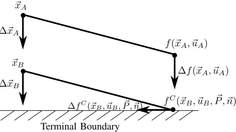
Terminal Boundary

~ xA

f(~xA, ~uA)

∆~xA

~ xB

fC_(~x

B, ~uB, ~P , ~n)

∆~xB

∆f(~xA, ~uA)

∆fC(~xB, ~uB, ~P , ~n)

Fig. 5: This diagram shows how the derivatives of the model function f(~x, ~u) radically change as the agent approaches a terminal boundary. The straight line segment from ~xA to

f(~xA, ~uA) represents a state transition that is not

intersect-ing the terminal boundary. If the start of this line segment is perturbed in the direction of the arrow ∆~xA then its

other end will move in the direction indicated by the arrow

∆f(~xA, ~uA). The line segment below, however, which starts

at ~xB, does reach the terminal boundary. If the start of this

line segment is moved in the direction of ∆~xB, then its end

will move in a perpendicular direction, as indicated by the arrow ∆fC(~xB, ~uB, ~P , ~n). This indicates that ∂fC/∂~x

A is

very different from (∂f /∂~x)_B, and hence this needs treating carefully in the ADP algorithms.

that are dependent on ∂fC_{/∂~xare critically affected by the}

need for clipping, and also that just reducing the duration of each time step tracking or simulating the motion will not solve the problem at all.

Differentiating the formula for S(~x, ~u, ~P , ~n)in (11) gives:

∂S(~x, ~u, ~P , ~n)

∂~x = ∂ ∂~x

(P~−~x)·~n

(f(~x, ~u)−~x)·~n

!

by (11)

= −~n

~ v·~n−

(P~−~x)·~n

(~v·~n)2

∂(f(~x, ~u)−~x)·~n ∂~x

using (10)

= −~n

~ v·~n−

(P~−~x)·~n

(~v·~n)2

_∂f

∂~x−I

~

n (15) where I is the identity matrix, and the matrix notation is as defined in Section II-A. Similarly,

∂S(~x, ~u, ~P , ~n)

∂~u = ∂ ∂~u

(P~ −~x)·~n

(f(~x, ~u)−~x)·~n

!

by (11)

=−(

~

P−~x)·~n

(~v·~n)2

∂(f(~x, ~u)−~x)·~n

∂~u using (10)

=−(

~

P−~x)·~n

(~v·~n)2

_∂f

∂~u

~

n (16) Using these derivatives of S(~x, ~u, ~P , ~n), we can now dif-ferentiate the clipped model and cost functions, giving:

∂fC_{(~x, ~u, ~P , ~n)}

∂~x =I+ ∂S ∂~x~v

T _+s

_∂f

∂~x−I

by (10)-(12) (17)

∂fC(~x, ~u, ~P , ~n)

∂~u = ∂S ∂~u~v

T_+s∂f

∂~u by (10)-(12) (18) ∂UC_{(~x, ~u, ~P , ~n)}

∂~x = ∂S

∂~xU(~x, ~u) +s ∂U

∂~x by (13) (19) ∂UC_{(~x, ~u, ~P , ~n)}

∂~u = ∂S

∂~uU(~x, ~u) +s ∂U

∂~u by (13) (20)

The cost-to-go function for the penultimate time step, equa-tion (14), can be rewritten as a Q-funcequa-tion of both~x and~u, to give

Q(~xT−1, ~uT−1) :=UC(~xT−1, ~uT−1, ~P , ~n)

+γsΦ(fC(~xT−1, ~uT−1, ~P , ~n)). (21)

Differentiating this with respect to~uT−1 or ~xT−1 gives:

_∂Q

∂•

T−1

=

_∂UC

∂•

T−1

+γs

_∂fC

∂•

T−1

_∂Φ

∂~x

T

+ (lnγ)

_∂S

∂•

T−1

Φ(~xT)

!

(22)

where•represents either~uor ~x.

This equation, which relies upon the derivatives of

fC_{(~x, ~u, ~P , ~n) and U}C_{(~x, ~u, ~P , ~n) (as defined in equations}

(15) to (20)), can be used to modify BPTT from Alg. 1 into its corresponding “with clipping” version given in Alg. 5. Equation (22) appears in the algorithm directly in lines 9-10. The DHP and HDP algorithms need similar modifications to convert them to include clipping. Pseudocode for DHP with clipping is given in Alg. 6. In addition to those clipping modifications included in this algorithm, a further useful modification is line 4 which obviates the need for the “final critic update” line which appears in Alg. 2. This modification was included becauseGe(~x, ~w)can change discontinuously at the final time step of a trajectory, as indicated in Fig. 5, which would cause a small but unnecessary difficulty for learning by a smooth neural network.

Pseudocode for HDP with clipping can be generated by replacing the line “~xt+1←f(~xt, ~ut)” of Alg. 3 by lines 4-13

of Alg. 4, and replacing the line that calculates Qu by lines

5-14 of Alg. 5.

C. Implementing Clipping Efficiently and Correctly

To demonstrate how clipping would be correctly imple-mented with an ADP/RL algorithm, we use the BPTT al-gorithm for illustration. In an implementation of BPTT with clipping, we would first evaluate a trajectory by Alg. 4. During this stage, we would record the full trajectory(~x0, ~x1, . . . , ~xT)

and actions(~u0, ~u1, . . . , ~uT−1)and also, during the collision

with the terminal boundary, we would recordP~ and~nand the clipping fraction, s. We then have enough information to be able to run the BPTT algorithm with clipping (Alg. 5).

To ensure the correctness of our implementations in each experiment and environment which we tackled, we first veri-fied all of the derivatives ofS(~x, ~u, ~P , ~n),fC_{(~x, ~u, ~P , ~n)and}

Algorithm 5Backpropagation Through Time for Control, with Clipping.

1: Unroll full trajectory from start state~x0using Alg. 4, and

retain the variables~xt,~ut,T,s,P~ and~n.

2: ∂J /∂~z←~₀

3: ~p←(∂Φ/∂~x)_T

4: fort=T−1 to0step −1 do 5: if~xt+1∈T then

6: Calculate(∂S/∂~x)_tand(∂S/∂~u)_tby (15) and (16).

7: Calculate ∂fC/∂~x_t and ∂fC/∂~u_t by (17) and (18).

8: Calculate ∂UC/∂~x_t and ∂UC/∂~u_t by (19) and (20).

9: Qx← ∂UC/∂~x

t

+γs _∂fC_/∂~x

t~p+ (lnγ) (∂S/∂~x)tΦ(~xT)

10: Qu← ∂UC/∂~u_t

+γs ∂fC/∂~u_t~p+ (lnγ) (∂S/∂~u)_tΦ(~xT)

11: else

12: Qx←(∂U /∂~x)t+γ(∂f /∂~x)t~p

13: Qu←(∂U /∂~u)t+γ(∂f /∂~u)t~p

14: end if

15: ∂J /∂~z←∂J /∂~z+γt_(∂A/∂~z) tQu

16: ~p←Qx+ (∂A/∂~x)_tQu

17: end for

18: ~z←~z−α(∂J /∂~z)

Algorithm 6 DHP with Clipping.

1: t←0

2: while~xt∈/Tdo

3: Evaluate~xt+1, with clipping, by lines 3-13 of Alg. 4.

4: ~p←

(

(∂Φ/∂~x)_t+1 if~xt+1∈T

e

G(~xt+1, ~w) if~xt+1∈/T

5: CalculateQx andQu by lines 5-14 of Alg. 5.

6: ~e←Qx+ (∂A/∂~x)tQu−Ge(~xt, ~w)

7: w~ ←w~ +β∂G/∂ ~e w

t

~e{Critic network update} 8: ~z←~z−α(∂A/∂~z)_tQu {Action network update}

9: t←t+ 1

10: end while

numerical differentiation that the overall BPTT implementa-tion was calculating the derivative ∂J_∂~zC correctly.

For an example of the numerical differentiations used, the final check of BPTT was done by a central-differences numerical derivative for each componentiof the weight vector

~

z, to verify that

∂JC ∂~zi =

JC(~x0, ~z+~ei)−JC(~x0, ~z−~ei)

2 +O(

2₎

whereis a small positive constant, and~eiis theith Euclidean

standard basis vector. In this verification equation, eachJC(·)

term appearing in the right-hand side would be computed by executing Alg. 4 from the trajectory start point ~x0; and the

theoretical value of ∂JC/∂~z appearing in the left-hand side would be computed by Alg. 5. Automated unit-test scripts were used in our implementation, to calculate these numerical

derivatives and successfully check the correctness of all stages of the clipping algorithm, and of all derivative calculations.

In HDP and DHP, the derivatives of S(~x, ~u, ~P , ~n),

fC_{(~x, ~u, ~P , ~n) and U}C_{(~x, ~u, ~P , ~n) would be calculated and}

verified as above. However with HDP and DHP it is more difficult to check the overall critic weight updates numerically, since they are not true gradient descent on any analytic function [30]. For these algorithms, it is still possible to verify the key algorithmic modifications related to clipping, by just checking the derivatives of the Q-function given by (22). These derivatives can be compared to the numerical derivatives of (21) with respect to~xand~u.

D. Clipping with Trajectories of Fixed or Variable Length

In situations where trajectories are of predetermined fixed length, clipping is not necessary. This is in contrast to the problems considered in the introduction, which were variable-length problems, since the trajectory variable-lengths were determined by the environment (e.g. a trajectory terminates only when the agent crashes into a wall). In this section we will consider the difference between these two types of episodic problem, i.e. between fixed-length and variable-length problems. Only in variable-length problems is clipping necessary.

In the fixed-length problem, the clipping fraction defined by (11) is alwayss≡1, and therefore ∂S/∂~x=~0, ∂S/∂~u=~0

and γs _{= γ. Hence the clipped model and cost functions}

are identical to their unclipped counterparts, and therefore it is not necessary to implement any program code specifically to handle clipping. This might be one reason why the need for clipping has not previously been noted in the research literature, since most episodic problems considered have been fixed-length.

However the fixed-length problem does have one minor different complication, in that it is often necessary to include the time step into the state vector. This is because the optimal actions and cost-to-go function will often be dependent upon the number of incomplete steps in a trajectory.

Of course for both fixed-length and variable-length prob-lems, it is important to ensure the terminal cost functionΦ(~x)

is learnt correctly by the learning algorithm. The pseudocode shows explicitly how to do this (e.g. for BPTT, see line 2 of Alg. 1, or line 3 of Alg. 5. For DHP and HDP, see lines commented as “final critic update”, and line 4 of Alg. 6.)

IV. A NOTE ONPOLICY-GRADIENTMETHODS

As we have seen, BPTT is an algorithm which can be used for gradient descent on the total cost-to-go function

J(~x, ~z)with respect to ~z. Another class of algorithms which do something similar are Policy-Gradient Learning (PGL) methods. These include the REINFORCE algorithm by [22], plus related methods (e.g. [23]). PGL methods are stochastic algorithms which do gradient descent of the form

h∆~zi=−α∂hJi

∂ ~w , (23)

wherehidenotes expectation.

model or cost functions, and thus are not affected by the need for clipping. For example, the REINFORCE weight update is defined, for trajectories of length one, to be:

∆~z=−α∂ln(g(~u0|~x0, ~z))

∂~z (U(~x0, ~u0)−b)

=−α 1 g(~u0|~x0, ~z)

∂g(~u0|~x0, ~z)

∂~z (U(~x0, ~u0)−b) (24)

whereα >0is small learning-rate constant, andbis a constant “baseline” scalar, and g(~u0|~x0, ~z)is a probability distribution

that forms the policy, such that action~u0is randomly sampled

from this distribution, and the distribution g(~u0|~x0, ~z) is

modelled by a function approximator with weight vector ~z

and input ~x0. Clearly this weight update (24) includes no

derivatives of f(~x, ~u), and hence has no need for clipping. However the expectation of this weight update is proven by [22] to be equivalent to (23), for any choice of the baseline constant.

The BPTT weight update is∆~z=−α(∂J /∂ ~w). In stochas-tic environments, the BPTT weight update would therefore average to

h∆~zi=−α

_∂J

∂ ~w

. (25) The derivation of the BPTT algorithm, in Section II-A, shows that this algorithm does require derivatives of f(~x, ~u), and hence does require clipping.

So how do we reconcile that for two such similar algorithms, BPTT requires clipping, but PGL does not? The answer lies in the subtle difference between equations (23) and (25), i.e. the fact that in general, the derivative of a mean can be different from the mean of a derivative. In the PGL case, the hJi

term has a blurring effect which first smoothes out all of the jagged bumps in the J versus ~z graph (for example as shown in Fig. 2b), and then PGL performs gradient descent on this blurred-out graph. In contrast, BPTT first calculates the gradient of various randomly chosen points of this graph, and then averages out the answer, and clearly in the case of Fig. 2b, this approach will not work (unless clipping is done). This shows that PGL methods have an advantage over BPTT methods in avoiding the need for clipping. However this complements the natural advantages that BPTT has over PGL, which are that BPTT can accumulate a learning gradient in just one trajectory, and therefore every single weight update provides useful learning. In contrast, PGL must form the mean from many weight updates before it can learn anything useful. In fact, a major area of research for PGL methods is to reduce the variance in these stochastic weight updates, so that the mean forms faster [23].

Other differences between the methods are that PGL is a model-free algorithm, whereas BPTT is model-based and requires knowledge of the functionf(~x, ~u)and its derivatives. A flip side of being model-based, is that when BPPT is used, trajectories automatically bend themselves into locally optimal shapes, but the model-free PGL methods require explicit (and usually stochastic) exploration of the environment to achieve this. Finally, BPTT requires that the functionJ(~x, ~z)

is reasonably smooth with respect to ~z for gradient-descent

methods to work well, but PGL methods do not have this requirement. PGL methods are resilient against roughness of theJ(~x, ~z)surface, due to the aforementioned blurring effect of the expectation operator on hJi. PGL’s ability to cope without clipping is an example of this resiliance.

To summarise, it is clear that the rival methods of BPTT and PGL have multiple relative pros and cons, and it is good to be aware of all of these issues.

V. EXPERIMENTALRESULTS

This section describes two neural-network based ADP/RL control problems which require clipping to be solved well.

In all experiments the action and critic networks used were multi-layer perceptrons (MLPs, see [31] for details). Each MLP haddim(~x)input nodes, 2 hidden layers of 6 nodes each, and one output layer, with short-cut connections connecting all pairs of layers. The output layers were dimensioned as follows: Each action network haddim(~u)output nodes; each HDP critic network had 1 output node; and each DHP critic haddim(~x)output nodes. All network nodes had bias weights, as is usual in MLP architectures. The activation functions used were hyperbolic tangent functions, except for the critic network’s output layer which was always a linear activation function (with linear slope as specified in the individual experiments, below). At the start of each experimental trial, neural weights were initialised randomly in the range[−.1, .1], with uniform probability distribution.

A. Vertical-Lander problem

A spacecraft is dropped in a uniform gravitational field, and its objective is to make a fuel-efficient gentle landing. The spacecraft is constrained to move in a vertical line, and a single thruster is available to make upward accelerations. The state vector~x= (xh, xv, xf)T has three components: height (xh),

velocity (xv), and fuel remaining (xf). The action vector,a, is

one-dimensional (so that~u≡a∈R) producing accelerations

a ∈ [0,1]. The Euler method with time-step ∆τ is used to integrate the motion, giving model functions:

f((xh, xv, xf)T, a) :=(xh+xv∆τ, xv+ (a−kg)∆τ,

(ku)xf−a∆τ)T

U((xh, xv, xf)T, a) :=(kf)a∆τ (26)

Here,kg= 0.2 is a constant giving the acceleration due to

gravity; the spacecraft can produce greater acceleration than that due to gravity.kf = 4 is a constant giving fuel penalty.

ku= 1is a unit conversion constant. We used∆τ= 1in our

main experiments here.

Trajectories terminate as soon as the spacecraft hits the ground (xh = 0) or runs out of fuel (xf = 0). These two

conditions define T. This is a variable-length problem, and

there is no need to use a discount factor, so we fixed γ= 1. On termination, the algorithms need to choose values for P~

(i.e the one that produces a smaller clipping fraction by (11)) is to be used.

In addition to the cost function U(~x, a) defined above, a final impulse of cost defined by,

Φ(~xT) :=

1 2m(xv)

2

+m(kg)xh, (27)

is given as soon as the lander reaches a terminal state, where

m = 2 is the mass of the spacecraft. The two terms in the final impulse of cost are the kinetic and potential energy, respectively. The first cost term penalises landing too quickly. The second term is a cost term equivalent to the kinetic energy that the spacecraft would acquire by crashing to the ground under free fall (i.e. with a= 0), so to minimise this cost the spacecraft must learn to not run out of fuel.

The input vector to the action and critic networks was~x0= (xh/100, xv/10, xf/50)

T

, and the model and cost functions were redefined to act on this rescaled input vector directly. The action network’s output ywas rescaled to give the action by A(~x, ~z) := (y+ 1)/2 directly. We tested each algorithm in batch mode, operating on five trajectories simultaneously. Those five trajectories had fixed start points, which had been randomly chosen in the regionxh∈(0,100),xv∈(−10,10)

andxf = 30.

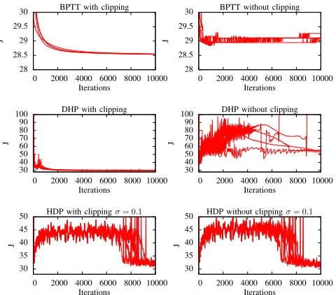
Fig. 6 shows learning performance of the BPTT, DHP and HDP algorithms, both with and without clipping. Each graph shows five curves, and each curve shows the learning performance from a different random weight initialisation. The learning rates for the three algorithms were: BPTT (α= 0.01); DHP (α = 0.001, β = 0.00001); and HDP (α = 0.00001,

β = 0.00001). The critic-network’s output layer’s activation function had a linear slope of 20 in the DHP experiment and 10 in the HDP experiment. In BPTT and DHP, the true derivatives of equations (26)-(27) were used where needed.

Because HDP is an algorithm which requires stochastic exploration to optimise the ADP/RL problem effectively [32], in the HDP experiment we had to modify (3) to choose exploratory actions. Hence for the HDP experiment we used

~

ut=A(~xt, ~z) +Xσ, (28)

whereXσis a normally distributed random variable with mean

zero and standard deviation σ= 0.1.

These graphs show the clear stability and performance advantages of using clipping correctly for the BPTT and DHP algorithms. The graphs also confirm that the HDP algorithm is not significantly affected by the need for clipping. The reason that clipping is important for BPTT and DHP is illustrated in Fig. 8.

Fig. 7 shows that the need for clipping is not diminished just by using a smaller ∆τ value.

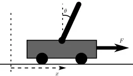
B. Cart-Pole Experiment

We investigated the effects of clipping in the well known cart-pole benchmark problem described in Fig. 9. We con-sidered the version of this problem used by [33], where the total trajectory cost is a function of the duration that the pole could be balanced for. Clearly, unless clipping is used properly, the duration will be an integer number of time steps,

28 28.5 29 29.5 30

0 2000 4000 6000 8000 10000

J

Iterations BPTT with clipping

28 28.5 29 29.5 30

0 2000 4000 6000 8000 10000

J

Iterations BPTT without clipping

30 40 50 60 70 80 90 100

0 2000 4000 6000 8000 10000

J

Iterations DHP with clipping

30 40 50 60 70 80 90 100

0 2000 4000 6000 8000 10000

J

Iterations DHP without clipping

30 35 40 45 50

0 2000 4000 6000 8000 10000

J

Iterations HDP with clippingσ= 0.1

30 35 40 45 50

0 2000 4000 6000 8000 10000

J

Iterations HDP without clippingσ= 0.1

Fig. 6: Vertical-Lander solutions by BPTT, DHP and HDP using ∆τ = 1. Each graph shows five curves, i.e. five experimental trials.

28 28.5 29 29.5 30

0 2000 4000 6000 8000 10000

J

Iterations BPTT with clipping∆t= 0.01

28 28.5 29 29.5 30

0 2000 4000 6000 8000 10000

J

Iterations BPTT without clipping∆t= 0.01

Fig. 7: Vertical Lander with ∆τ = 0.01. Each graph shows five curves, i.e. five experimental trials.

and since this is not smooth and differentiable, it will cause problems (become impossible) for DHP and BPTT. Hence traditionally when DHP or BPTT are used for the cart-pole problem, a different cost function would be used, one that is differentiable and proportional to the deviation from the balanced position (e.g. see [34]). However in this section we show that by using clipping, DHP and BPTT can be successful with the duration-based reward. Since it is not possible to do this without clipping, we assume this is the first published version of this solution by DHP/BPTT.

The equation of motion for the frictionless cart-pole system ( [33]–[35]) is:

¨

θ=

gsinθ−cosθhF+mlθ˙2sinθ mc+m

i

lh4 3−

mcos2_θ

mc+m

i (29)

TABLE I: Terminal Boundary Planes used in vertical-lander experiment. The state vector used here is~x= (xh, xv, xf)T.

xv

xh

Fig. 8: The tail end of an optimal trajectory in the vertical-lander problem. As the spacecraft lands gently, it increases the velocity (xv) as it approaches the ground (xh= 0), hence

making the curved trajectory shown. As the trajectory curve approaches the terminal boundary, clipping affects the gradient

∂fC/∂~xas shown in Fig. 5, and hence this twists the gradient

∂JC_{/∂~xdiscontinuously at the terminal state~x} T.

F θ

x

Fig. 9: Cart-pole benchmark problem. A pole with a pivot at its base is balancing on a cart. The objective is to apply a changing horizontal force F to the cart which will move the cart backwards and forwards so as to balance the pole vertically. State variables are pole angle,θ, and cart position,

x, plus their derivatives with respect to time,θ˙ andx˙.

¨

x=

F+mlhθ˙2_sinθ−θ¨_cosθi

mc+m

(30)

where gravitational acceleration, g = 9.8ms−2; cart’s mass,

mc = 1kg; pole’s mass, m = 0.1kg; half pole length,

l = 0.5m; F ∈ [−10,10] is the force applied to the cart, in Newtons; and the pole angle, θ, is measured in radians. The motion was integrated using the Euler method with a time con-stant ∆τ = 0.02, which, for a state vector ~x≡(x, θ,x,˙ θ˙)T_,

gives a model function f(~x, ~u) =~x+ ( ˙x,θ,˙ x,¨ θ¨)T_∆τ.

The pole motion continues until it reaches a terminal state or until the pole is successfully balanced for 300 time steps, i.e. 6 seconds of real time. Terminal states (T) are defined to

be any state with |x| ≥2.4, or|θ| ≥ π

15 (i.e. 12 degrees), or

t≥300. Termination plane constants are given in Table II. The duration-based cost function of [33] is equivalent to

U(~x, u) := 0, (31)

TABLE II: Terminal Boundary Planes used in cart-pole exper-iment. The state vector used here is~x= (x,x, θ,˙ θ, t˙ )T.

Termination Position Vector Normal Vector Condition Breached of Plane,P~T _{to Plane,~n}T θ≥π/15 (0,0,π/15,0,0) (0,0,−1,0,0) θ≤ −π/15 (0,0,−π/15,0,0) (0,0,1,0,0) x≥2.4 (2.4,0,0,0,0) (−1,0,0,0,0) x≤ −2.4 (−2.4,0,0,0,0) (1,0,0,0,0) t≥300 (0,0,0,0,300) (0,0,0,0,1)

for non-terminal states, and,

Φ(~x) :=

(

1 ifT <300,

0 otherwise, (32)

for terminal states~x∈T. When the above two cost functions

are used in conjunction with a discount factor γ < 1, and when the pole eventually falls over (i.e. when T <300), the total trajectory cost isJ(~x0, ~z)≡γT, whereT is the time at

which the trajectory terminated. Since this function decreases withT, minimising it will increaseT, i.e. lead to successful pole balancing.1

We tested the three algorithms BPTT, DHP and HDP on this problem with a discount factor γ = 0.97. To en-sure the state vector was suitably scaled for input to the MLPs, we used rescaled state vectors ~x0 defined by ~x0 = (0.16x,15θ/π,x,˙ 4 ˙θ, t/300)T_{, with θ in radians, throughout}

the implementation. As noted by [34], choosing an appropriate state-space scaling can be critical to successful convergence of actor-critic architectures in the cart-pole problem. Note that our implementation also uses the time step t as an input to the neural network, since the cost-to-go function that is being learned does depend upon t. The output of the action network, y, was multiplied by 10 to give the control force

F =A(~x, ~z) := 10y. The learning rates for the algorithms that we used were: BPTT (α= 0.1); DHP (α= 0.001,β= 0.01); HDP (α= 0.01,β = 0.1). The DHP and HDP critics used a final-layer activation-function slope of 0.1. HDP used a policy exploration rate of σ = 0.15 (using (28)), and the other algorithms used σ = 0. The exact derivatives of the model and cost functions were made available to the algorithms.

During learning, each trajectory was defined to start at the point x = 0, θ = 0, x˙ = 0.4, θ˙ = 0. This is a start state from which the pole will quickly topple over, unless corrective control actions are taken.

The performance of the three algorithms, both with and without clipping, are shown in Fig. 10. Each graph shows the balancing duration versus the training iteration, for an ensemble of five different curves, with each curve representing a training run from a different random weight initialisation.

The results show that using clipping correctly enables both the DHP and BPTT algorithms to solve this problem consistently, and without clipping it is impossible for both algorithms. The results show that HDP is largely unaffected by clipping.

This problem is interesting in that the cost functions defined by (31) and (32) would be completely inappropriate for learn-ing with BPTT/DHP unless clipplearn-ing is used correctly, since they have zero derivatives everywhere, i.e. (∂Φ/∂~x)_T ≡~_0, ∂U /∂~u ≡ ~_{0 and ∂U /∂~x ≡} ~_{0. The clipping algorithm}

solves this problem through the expression in (22) given by

(lnγ) (∂S/∂•)_T−1Φ(~xT), which appears in lines 9-10 of Alg.

5. This expression allows for a useful learning gradient to be

1_{Previously, other researchers may have usedΦ(~x) := 1 instead of our}

0 50 100 150 200 250 300 350 400

0 200 400 600 800 1000

T

rajectory

Duration

Iterations BPTT with clipping

0 50 100 150 200 250 300 350 400

0 200 400 600 800 1000

T

rajectory

Duration

Iterations BPTT without clipping

0 50 100 150 200 250 300 350 400

0 1000 2000 3000 4000 5000

T

rajectory

Duration

Iterations DHP with clipping

0 50 100 150 200 250 300 350 400

0 1000 2000 3000 4000 5000

T

rajectory

Duration

Iterations DHP without clipping

0 50 100 150 200 250 300 350 400

0 50 100 150 200

T

rajectory

Duration

Iterations (×1000) HDP with clipping

0 50 100 150 200 250 300 350 400

0 50 100 150 200

T

rajectory

Duration

Iterations (×1000) HDP without clipping

Fig. 10: Cart-pole solutions by BPTT, DHP and HDP. Each graph shows five curves, i.e. five experimental trials.

obtained. For it to work, we must have ln(γ) 6= 0, which requires that γ <1, and also we must have Φ(~xT)6= 0.

Fur-thermore, the derivatives of the clipping fraction, i.e. ∂S/∂~x

and∂S/∂~u, must be calculated correctly by (15) and (16) for the pole-balancing problem to be solved.

VI. CONCLUSIONS

The problem of clipping for ADP/RL and neurocontrol algorithms has been demonstrated and motivated. Without clipping, algorithms which rely on the derivatives of the model and cost functions can fail to work. The solution is to apply clipping, and then to correctly differentiate the model and cost functions in the final time step. This solution has been given in the form of the equations, plus in the form of clear pseudocode for the two major affected ADP algorithms: DHP and BPTT. Two neural-network experiments have confirmed the impor-tance of applying clipping correctly. These included a cart-pole experiment, where clipping was found to be essential, and in a vertical-lander experiment, where clipping produced a significant improvement of performance.

The situations in which clipping is needed have been made clear, and those situations where it can be ignored have also been specified.

REFERENCES

[1] F.-Y. Wang, H. Zhang, and D. Liu, “Adaptive dynamic programming: An introduction,”IEEE Computational Intelligence Magazine, vol. 4, no. 2, pp. 39–47, 2009.

[2] P. J. Werbos, “Neurocontrol: Where it is going and why it is crucial,” inArtifical Neural Networks II (ICANN-2), North Holland, Amsterdam, I. Aleksander and J. Taylor, Eds., 1992, pp. 61–68.

[3] M. Hagan and H. Demuth, “Neural networks for control,” inAmerican Control Conference, 1999. Proceedings of the 1999, vol. 3. IEEE, 1999, pp. 1642–1656.

[4] R. S. Sutton and A. G. Barto,Reinforcement Learning: An Introduction. Cambridge, Massachussetts, USA: The MIT Press, 1998.

[5] F. L. Lewis, D. Vrabie, and K. G. Vamvoudakis, “Reinforcement learning and feedback control: Using natural decision methods to design optimal adaptive controllers,”Control Systems, IEEE, vol. 32, no. 6, pp. 76–105, 2012.

[6] P. J. Werbos, “Approximating dynamic programming for real-time control and neural modeling.” inHandbook of Intelligent Control, D. A. White and D. A. Sofge, Eds. New York: Van Nostrand Reinhold, 1992, ch. 13, pp. 493–525.

[7] D. Prokhorov and D. Wunsch, “Adaptive critic designs,”IEEE Transac-tions on Neural Networks, vol. 8, no. 5, pp. 997–1007, 1997. [8] P. J. Werbos, “Backpropagation through time: What it does and how to

do it,” inProceedings of the IEEE, vol. 78, No. 10, 1990, pp. 1550–1560. [9] M. Fairbank and E. Alonso, “Value-gradient learning,” inProceedings of the IEEE International Joint Conference on Neural Networks 2012 (IJCNN’12). IEEE Press, June 2012, pp. 3062–3069.

[10] M. Fairbank, D. Prokhorov, and E. Alonso, “Approximating optimal control with value gradient learning,” in Reinforcement Learning and Approximate Dynamic Programming for Feedback Control, F. Lewis and D. Liu, Eds. New York: Wiley-IEEE Press, 2012, pp. 142–161. [11] M. Fairbank, “Reinforcement learning by value gradients,”CoRR, vol.

abs/0803.3539, 2008. [Online]. Available: http://arxiv.org/abs/0803.3539 [12] M. Fairbank, E. Alonso, and D. Prokhorov, “An equivalence between adaptive dynamic programming with a critic and backpropagation through time,” IEEE Transactions on Neural Networks and Learning Systems, vol. 24, no. 12, pp. 2088–2100, December 2013.

[13] D. Prokhorov, “Backpropagation through time and derivative adaptive critics: A common framework for comparison,” inHandbook of learning and approximate dynamic programming, J. Si, A. Barto, W. Powell, and D. Wunsch, Eds. New York: Wiley-IEEE Press, 2004.

[14] M. Fairbank and E. Alonso, “The local optimality of reinforcement learning by value gradients, and its relationship to policy gradient learning,” CoRR, vol. abs/1101.0428, 2011. [Online]. Available: http://arxiv.org/abs/1101.0428

[15] R. Munos, “Policy gradient in continuous time,” Journal of Machine Learning Research, vol. 7, pp. 413–427, 2006.

[16] M. Fairbank, E. Alonso, and D. Prokhorov, “Simple and fast calculation of the second-order gradients for globalized dual heuristic dynamic pro-gramming in neural networks,”IEEE Transactions on Neural Networks and Learning Systems, vol. 23, no. 10, pp. 1671–1678, October 2012. [17] M. Abu-Khalaf and F. L. Lewis, “Nearly optimal control laws for

nonlinear systems with saturating actuators using a neural network HJB approach,”Automatica, vol. 41, no. 5, pp. 779–791, 2005.

[18] A. Al-Tamimi, M. Abu-Khalaf, and F. L. Lewis, “Adaptive critic designs for discrete-time zero-sum games with application toh∞control.”IEEE Transactions on Systems, Man, and Cybernetics, Part B: Cybernetics, vol. 37, no. 1, pp. 240–247, February 2007.

[19] A. Al-Tamimi, F. L. Lewis, and M. Abu-Khalaf, “Discrete-time non-linear HJB solution using approximate dynamic programming: Conver-gence proof.” IEEE Transactions on Systems, Man, and Cybernetics, Part B, vol. 38, no. 4, pp. 943–949, 2008.

[20] H. Zhang, Y. Luo, and D. Liu, “Neural-network-based near-optimal control for a class of discrete-time affine nonlinear systems with control constraints,”Neural Networks, IEEE Transactions on, vol. 20, no. 9, pp. 1490–1503, 2009.

[21] H. Zhang, Q. Wei, and Y. Luo, “A novel infinite-time optimal tracking control scheme for a class of discrete-time nonlinear systems via the greedy HDP iteration algorithm,”Systems, Man, and Cybernetics, Part B: Cybernetics, IEEE Transactions on, vol. 38, no. 4, pp. 937–942, 2008. [22] R. J. Williams, “Simple statistical gradient-following algorithms for connectionist reinforcement learning,” Machine Learning, vol. 8, pp. 229–356, 1992.

[23] J. Peters and S. Schaal, “Policy gradient methods for robotics,” in Proceedings of the IEEE/RSJ International Conference on Intelligent Robots and Systems (IROS), 2006.

[24] C. J. C. H. Watkins, “Learning from delayed rewards,” Ph.D. disserta-tion, Cambridge University, 1989.

[25] S. Ferrari and R. F. Stengel, “Model-based adaptive critic designs,” in Handbook of learning and approximate dynamic programming, J. Si, A. Barto, W. Powell, and D. Wunsch, Eds. New York: Wiley-IEEE Press, 2004, pp. 65–96.

[26] R. S. Sutton, “Learning to predict by the methods of temporal differ-ences,”Machine Learning, vol. 3, pp. 9–44, 1988.

[27] K. Doya, “Reinforcement learning in continuous time and space,”Neural Computation, vol. 12, no. 1, pp. 219–245, 2000.

[29] D. E. Rumelhart, G. E. Hintont, and R. J. Williams, “Learning repre-sentations by back-propagating errors,”Nature, vol. 323, no. 6088, pp. 533–536, 1986.

[30] E. Barnard, “Temporal-difference methods and markov models,”IEEE Transactions on Systems, Man, and Cybernetics, vol. 23, no. 2, pp. 357– 365, 1993.

[31] C. M. Bishop, Neural Networks for Pattern Recognition. Oxford University Press, 1995.

[32] M. Fairbank and E. Alonso, “A comparison of learning speed and ability to cope without exploration between DHP and TD(0),” inProceedings of the IEEE International Joint Conference on Neural Networks 2012 (IJCNN’12). IEEE Press, June 2012, pp. 1478–1485.

[33] A. G. Barto, R. S. Sutton, and C. W. Anderson, “Neuronlike adaptive elements that can solve difficult learning control problems,” IEEE Transactions on Systems, Man, and Cybernetics, vol. 13, pp. 834–846, 1983.

[34] G. G. Lendaris and C. Paintz, “Training strategies for critic and action neural networks in dual heuristic programming method,” inProceedings of International Conference on Neural Networks, Houston, 1997. [35] R. V. Florian, “Correct equations for the dynamics of the cart-pole

system,” Center for Cognitive and Neural Studies (Coneural), Str. Saturn 24, 400504 Cluj-Napoca, Romania, Tech. Rep., 2007.

Michael Fairbankreceived his BSc degree in Math-ematical Physics from Nottingham University in 1994, and MSc in Knowledge Based Systems from Edinburgh University in 1995. He has been inde-pendently researching ADPRL and neural networks since that time, while pursing careers in computer programming and mathematics teaching. He is now a PhD student at City University London.

His research interests include neurocontrol, ADP methods (particularly DHP, VGL(λ) and BPTT), and neural-network learning algorithms (especially for recurrent neural networks).

Dr. Danil Prokhorov (SM02) began his career in St. Petersburg, Russia, in 1992. He was a research engineer in St. Petersburg Institute for Informatics and Automation of the Russian Academy of Sci-ences. He became involved in automotive research in 1995 when he was a Summer intern at Ford Scientific Research Lab in Dearborn, MI. In 1997 he became a Ford Research staff member involved in application-driven research on neural networks and other machine learning methods. While at Ford, he was involved in several production-bound projects including neural network based engine misfire detection. Since 2005 he is with Toyota Technical Center, Ann Arbor, MI. He is currently in charge of Mobility Research Department with Toyota Research Institute North America, a TTC division. He has more than 100 papers in various journals and conference proceedings, as well as several inventions, to his credit. He is honored to serve in a number of capacities including the International Neural Network Society (INNS) President, the National Science Foundation (NSF) Expert, and the Associate Editor/Program Committee member of many international journals/conferences.