Comparison of Two Methods Cost and Reliability for Components in Architecture based Software System using Dynamic Programming

(1)

Comparison of Two Methods Cost and Reliability for

Components in Architecture-based Software System using

Dynamic Programming

Srinivasarao.Sabbineni

Assistant Professor,

Computer Science and Engineering Department, K.L.University,Vaddeswaram,

Guntur,Andhrapradesh State -522502, India

Kurra.Rajasekhara Rao,

Ph.D

Professor,

Computer Science and Engineering Department, K.L.University,Vaddeswaram,

Guntur,Andhrapradesh State -522502, India

ABSTRACT

In an architecture-based software system Reliability allocation to different sizes of components plays a major role throughout the software product design phase, which has close relation ship with cost and reliability of software. In this paper dynamic programming algorithm is used to allocate the reliability and cost of each component for designing software using step length .Here we applied both minimum step length and maximum step length for allocation of reliability to different sizes of components. The result of our experiment show an optimal solution or near optimal to the problem of choosing the component containing the software can be achieved with lower cost.

Keywords

Architecture-based Software, Software Reliability, Reliability allocation, Dynamic programming, Software development, software model, Reliability Estimation

1. INTRODUCTION

The Software architecture is collected of components, connectors, and configurations. In design phase and implementation phase estimation of software total cost is very difficult. Software systems have a significant impact on our daily lives. Software failure is happened during operation of software can lead to economic loss and may even cause loss of human lives. That’s way unreliable software is not acceptable and should be identified in the starting stage of software development [1]. Later the defects found, the higher the cost that needs to be paid for them.

The discussion of this paper takes the following structure. Section 2 introduces software system reliability allocation model. Section 3 depicts find out the optimal allocation method by using a dynamic programming algorithm. Section 4 illustrates the application of the algorithm proposed in section 3 and section 5 offers conclusion and future work are presented.

2. SOFTWARE SYSTEM RELIABILITY

ALLOCATION MODEL:

2.1 Software system development cost

minimization versus maximizing reliability

allocation:

In fact, it is difficult to develop the software reliability while releasing the software system development cost because they are two inconsistent constraints. The invented software

development cost minimization can be measured from two facts of assessments[4]. One is to find an optimal reliability allocation method while achieving the given reliability such that the development cost can be as small as possible; the other is how to allocate the reliability to each component on the basis of the given cost so that the system reliability can be maximized. This paper focuses on the former one.

Several systems are executed by using a set of interconnected subsystems. Reliability allocation means fixing the reliability among different subsystems so that the total system development cost (including human, material resources, development time and testing time etc) can be minimized. Reliability allocation can be used to planning with such kind of problem that the goal is set prior to the solution. Normally the number of the solution is more than one, as a result reliability allocation is used to deal with the optimal problem with some restrictions.

2.2 Software reliability and cost model

It is reasonable to assume that the cost function fi. Would satisfy these three conditions.

•fi is a positive definite function

• fi is non-decreasing.

• fi increases at a higher rate for higher values of Ri

The third condition suggests that it can be very expensive to achieve the reliability value of 1.

According to the definition of software reliability;

r

(

t

)



e





t

--- (1)

where r(t) is continuous-time system reliability, λ is its failure rate.

According to the experience from practical engineering, this paper takes account of the factors by assuming that software reliability and development cost

Satisfithe relations as below:

1).Software development cost is inversely proportional to the number of system failures.

(2)





E

--- (3)

where C is the development cost and E is the number of system failures.using equation(2),reliability function (1) is therefore

C





1 /

ln

r

--- (4)

2.software development cost is proportional to the complexity and size of the software system.

Taking assumption 2) into account,the equation (4) can be expressed as:

C







/

ln

r

--- (5)

Where α represents the complexity size for developing the software system and is called reliability cost coefficient in this paper.

In consideration of the operation in practical engineering ,where personal training ,development tools preparation etc. we use character β to represent the basic development cost in this paper.

Reliability cost model as below:

C

(

r

)







/

ln

r





--- (6)

Equation(6) states the relationship between system development cost and system reliability in our mopdel.

Given a system with many components,the reliability of its component I can be also stated as:

C

(

R

_i

)





_i

/

ln

R

_i





_i --- (7)

2.3 Software reliability model

Here we assume the software system has been designed as an assembly of appropriated connected components. Let there be n components, each with reliability Ri and cost Ci,i=1,2…n.let Robj be the specified target reliability and the total system cost.Let F(R1,R2….Rm) be the function of R and Ri.

The software reliability allocation model can be stated as: Objective function

MinC

--- (8)

Subject to

r



F

(

r

₁

,

r

₂

,



r

_n

)



R

_obj

0 

r

_i



1

---- (9)

C





C

_i







_i







_i

/

ln

r

_i --- (10)

If β is simplified to 0(zero).then eq(10) can be rewriting as:

C





C

_i









_i

/

ln

r

_i --- (11)

within a given architecture ,the development system will increase while enhancing the software reliability target. Significantly, the greater improvement of the reliability ,the more increase of the cost will be required.

Such a problem can be resolved with variety methods,and dynamic programming is an option.

3. USING DYNAMIC PROGRAMMING

ALGORITHM TO SOLVE RELIABILITY

ALLOCATION PROBLEM:

A software system with n components and the association function F discussed above is known. The reliability-cost coefficient α of each component and the specified system reliability target R obj is given.

The dynamic programming algorithm is as follows:

Step 1: Let S represent the reliability matrix [r1,r2, ., rn], T represent the cost matrix [c1, c2, …, cn], δ be the solving step length, Ii represent the matrix with one column and n rows in which only the value of the ith element is 1 and the rest are all 0. Assume S0=[maxr, maxr, …, maxr], maxr represents the maximized possible reliability, for example 0.9999, which means the initial reliability values of the components are all maxr.

Step 2: As for S0, T0 can be solved(11), C0 can be given by and system reliability R0 can be given by function F.

Step 3: If R0<Robj then stop and return. No solutions.

Step 4: Set Rate=0;

Step 5: for i=1 to n

i) S’=S0 – Ii*δ;

ii) With regard to S’, Generate reliability R’ with the function F, T’ with (7), total cost C’ iii) ∆C= C0 - C’; ∆R= R0 – R’;

iv) if R’ ≥ Robj and ∆C/∆R >Rate then Set Rate=∆C/∆R , R=R’ , S=S’ , C=C’ , T=T’;

Step 6: if R0≠R then set S0=S; R0=R; C0=C; T0=T;

return to step 4

(3)

4. EXAMPLE AND RESULTS

Here we choose a system with three independent components r1, r2, r3. We assume that all the components are essential to the system and their failures are statistically independent. Therefore, the relationship between the total system reliability r and its components’ reliability ri (i=1, 2, 3) can be stated as: r = F (r1, r2, r3 ) = r1* r2* r3 Suppose that the complexities of the components are 0.45,0.82 and 0.64 respectively. In order to minimize the system development cost and the system reliability shall be no less than 0.95, how to allocate the reliability to each component. First method Set the precision of computing is 0.005.afeter completion of the first method take second method is for Set the precision of computing is 0.01.

Such a problem can be rewritten as:

First Method :

R＝r1* r2* r3≤0.95

C1= - 0.45/ln r1

C2= - 0.82/ln r2

C3= - 0.64/ln r3

Compute the values of parameters (r1, r2, r3) with which the total cost C (C＝c1+c2+c3) is minimized. With respect to each component, we compute the cost with the reliability from 0.95 to 0.995 (increment is 0.005) according to the reliability/cost function model in the data set as shown in Table 1.

According to the algorithm above, set initial state S0 = [0.995, 0.995, 0.995]. Accordingly, T0 = [89.77, 163.58, 127.67], δ=0.005, and the system cost C0=89.77+163.58+127.67 =381.02, system reliability R0= 0.995 * 0.995*0.995＝0.985.

Set i=1, 2, 3 then compute separately with different value:

1) S’= S0 – [0.005, 0, 0] = [0.99, 0.995, 0.995], R’=0.98, T’= [44.77, 163.58, 127.67], C’=336.02 ∆C=45, ∆R=0.005, ∆C/∆R=9000.

2) S’= S0 – [0, 0.005, 0] = [0.995, 0.99, 0.995], R’=0.98, T’= [89.77, 81.58, 127.67], C’=299.02 ∆C=82, ∆R=0.005,

∆C/∆R=16400.

3) S’= S0 – [0, 0, 0.005] = [0.995, 0.995, 0.99], R’=0.98, T’= [89.77, 163.58, 63.67], C’=317.02 ∆C= 64; ∆R=0.005, ∆C/∆R=12800.

Choose the optimal result 1), set S0=[0.99, 0.995, 0.995],continue to perform the same operation：

1) S’= S0 – [0.005, 0, 0] = [0.985, 0.995, 0.995], R’=0.975, T’= [29.27, 163.58, 127.67], C’=321.02, ∆C=15, ∆R=0.005, ∆C/∆R=3000

2) S’= S0 – [0, 0.005, 0] = [0.99, 0.99, 0.995], R’=0.975, T’= [44.77, 81.58, 127.67], C’=254.02 ∆C=82, ∆R=0.005, ∆C/∆R=16400

3) S’= S0 – [0, 0, 0.005] = [0.99, 0.995, 0.99], R’=0.975, T’= [44.77, 163.58, 63.67], C’=272.02 ∆C=64; ∆R=0.005, ∆C/∆R=12800

Choose the optimal result 2), set S0=[0.995, 0.99, 0.995], continue to perform the same operation：

1) S’= S0 – [0.005, 0, 0] = [0.99, 0.99, 0.995], R’=0.975, T’= [44.77, 81.58, 127.67], C’=254.02, ∆C=45, ∆R=0.005, ∆C/∆R=9000

2) S’= S0 – [0, 0.005, 0] = [0.995, 0.985, 0.995], R’=0.975, T’= [89.77, 54.25, 127.67], C’=271.69 ∆C=27.33, ∆R=0.005, ∆C/∆R=5466

Table 1: Cost and Reliability Dataset

3) S’= S0 – [0, 0, 0.005] = [0.995, 0.99, 0.99], R’=0.975, T’= [89.77, 81.58, 63.67], C’=235.02 ∆C=64; ∆R=0.005, ∆C/∆R=12800

Choose the optimal result 3),set S0=[0.995, 0.995, 0.99], continue to perform the same operation：

1) S’= S0 – [0.005, 0, 0] = [0.99, 0.995, 0.99], R’=0.975, T’= [44.77, 163.58, 63.67], C’=272.02, ∆C=45, ∆R=0.005, ∆C/∆R=9000

2) S’= S0 – [0, 0.005, 0] = [0.995, 0.99, 0.99], R’=0.975, T’= [89.77, 81.58, 63.67], C’=235.02 ∆C=82, ∆R=0.005, ∆C/∆R=16400

3) S’= S0 – [0, 0, 0.005] = [0.995, 0.995, 0.985], R’=0.975, T’= [89.77, 163.58, 42.34], C’=295.69 ∆C=21.33; ∆R=0.005, ∆C/∆R=4266

s.no r1 c1 r2 c2 r3 c3

1 0.95 8.77 0.95 15.98 0.95 12.47

2 0.955 9.77 0.955 17.80 0.955 13.89

3 0.96 11.02 0.96 20.08 0.96 15.67

4 0.965 12.63 0.965 23.01 0.965 17.96

5 0.97 14.77 0.97 26.92 0.97 21.01

6 0.975 17.77 0.975 32.38 0.975 25.27

7 0.98 22.27 0.98 40.58 0.98 31.67

8 0.985 29.77 0.985 54.25 0.985 42.34

9 0.99 44.77 0.99 81.58 0.99 63.67

(4)

[image:4.595.49.289.136.265.2]

all of the results R’ are less than the specified reliability target 0.95. Therefore, the reliability allocation in all cases is as below:

Table 2: Cost and Reliability Dataset

CASE (i):

1) System reliability allocation S0= [0.995, 0.995, 0.995];

2) System reliability R0=0.985;

3) Expected system development cost C0 = 299.02;

4) Expected development cost assigned to each components T0 = [89.77, 81.58, 127.67].

CASE (ii):

3) Expected system development cost C0 =254.02;

CASE (iii):

CASE (iv):

Second method:

Here we taken components sizes are same as in first method

R＝r1* r2* r3≤0.95

C1= - 0.45/ln r1

C2= - 0.82/ln r2

C3= - 0.64/ln r3

Compute the values of parameters (r1, r2, r3) with which the total cost C (C＝c1+c2+c3) is minimized. With respect to each component, we compute the cost with the reliability from 0.95 to 0.99 (increment is 0.01) according to the reliability/cost function model in the data set as shown in Table 1.

According to the algorithm above, set initial state S0 = [0.99, 0.99, 0.99]. Accordingly, T0 = [44.77, 81.58, 63.67], δ=0.01, and the system cost C0=44.77+81.58+63.67 = 190.02, system reliability R0= 0.99 * 0.99*0.99＝0.97.

Set i=1, 2, 3 then compute separately with different value:

1) S’= S0 – [0.01, 0, 0] = [0.98, 0.99, 0.99], R’=0.96, T’= [22.27, 81.58, 63.67], C’=167.52 ∆C=22.5, ∆R=0.01, ∆C/∆R=2250

2) S’= S0 – [0, 0.01, 0] = [0.99, 0.98, 0.99], R’=0.96, T’= [44.77, 40.58, 63.67], C’=149.02 ∆C=41, ∆R=0.01, ∆C/∆R=4100

3) S’= S0 – [0, 0, 0.01] = [0.99, 0.99, 0.98], R’=0.96, T’=

[44.77, 81.58, 31.67], C’=158.02 ∆C= 32; ∆R=0.01, ∆C/∆R=3200

Choose the optimal result 2), set S0=[0.99, 0.98, 0.99],continue to perform the same operation：

1) S’= S0 – [0.01, 0, 0] = [0.98, 0.98, 0.99], R’=0.95, T’= [22.27, 40.58, 63.67], C’=126.52, ∆C=22.5, ∆R=0.01, ∆C/∆R=2250

2) S’= S0 – [0, 0.01, 0] = [0.99, 0.97, 0.99], R’=0.95, T’= [44.77, 26.92, 63.67], C’=135.36 ∆C=13.66, ∆R=0.01, ∆C/∆R=1366

3) S’= S0 – [0, 0, 0.01] = [0.99, 0.98, 0.98], R’=0.95, T’= [44.77, 40.58, 31.67], C’=117.02 ∆C=32; ∆R=0.01, ∆C/∆R=3200

Choose the optimal result 3), set S0=[0.98, 0.99, 0.99], continue to perform the same operation：

1) S’= S0 – [0.01, 0, 0] = [0.97, 0.99, 0.99], R’=0.95, T’= [14.77, 81.58, 63.67], C’=160.02, ∆C=7.5, ∆R=0.01, ∆C/∆R=750

2) S’= S0 – [0, 0.01, 0] = [0.98, 0.98, 0.99], R’=0.95, T’= [22.27, 40.58, 63.67], C’=126.52 ∆C=41, ∆R=0.01, ∆C/∆R=4100

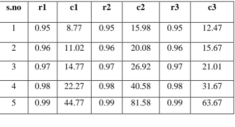
s.no r1 c1 r2 c2 r3 c3

1 0.95 8.77 0.95 15.98 0.95 12.47

2 0.96 11.02 0.96 20.08 0.96 15.67

3 0.97 14.77 0.97 26.92 0.97 21.01

4 0.98 22.27 0.98 40.58 0.98 31.67

(5)

[22.27, 81.58, 31.67], C’=135.52 ∆C=32; ∆R=0.01, ∆C/∆R=3200

Choose the optimal result 4),set S0=[0.99, 0.99, 0.98], continue to perform the same operation：

1) S’= S0 – [0.01, 0, 0] = [0.98, 0.99, 0.98], R’=0.95, T’= [44.77, 40.58, 31.67], C’=117.02, ∆C=41, ∆R=0.01, ∆C/∆R=4100

2) S’= S0 – [0, 0.01, 0] = [0.99, 0.98, 0.98], R’=0.94, T’= [34.82, 25.74, 73.63, 45.04], C’=179.23 ∆C=71.5, ∆R=0.01, ∆C/∆R=7150

3) S’= S0 – [0, 0, 0.01] = [0.99, 0.99, 0.97], R’=0.95, T’= [44.77, 81.58, 21.01], C’=147.36 ∆C=10.66; ∆R=0.01, ∆C/∆R=1066

all of the results R’ are less than the specified reliability target 0.95. Therefore, the reliability allocation in all cases is as below:

CASE (i):

CASE (ii):

CASE (iii):

CASE (iv):

5. CONCLUSION

Software reliability allocation to different sizes of system components throughout software product design phase and implementation phase which has close relationship with software modeling and cost estimation. We formulated an architecture-based style for showing software reliability optimization problem, on this basis a dynamic programming algorithm has been supported in this paper which can be used to allocate the reliability to every component so as to minimize the cost of designing software system components while meeting the chosen reliability independent. The result of our experiment display an optimal or approximate optimal solution to the problem of selecting the various sizes of components comprising software can be obtained with lower cost (a high reliability). This paper helps the comparison of setting the reliabilities to each component reliability and lower cost using any one method. These methods are used based on their requirement and based on step length they are using any one method. The reliability and cost allocation model presented in this paper can be used to solve the optimal allocation problems in simple and complex systems.

6. ACKNOWLEDGEMENTS

I state that in my research work, I am being guided by Dr.K.Rajasekhara Rao Professor, K.L.UNIVERSITY, Vaddeswaram, Guntur, and his guidance and support, I submitting research paper, which is a part of research work. I also acknowledge the support and encouragement given by University management and my family members and my friends and well-wishers to pursue the Research work.

7. REFERENCES

[1] Hui Guan,Tingmei Wang,Weiru Chen “Exploring Architecture-Based Software Reliability Allocation Using a D ynamic Programming Algorithm” Inproc.2nd symposium Int’l computer science and computational technology,Huangshan,P.R.China,26-28,Dec

.2009,pp.106-109.

[2] D.L.Parnas. “The Influence of Software Structure on Reliability”. In Proc.1975 Int’l Conf. Reliability software, Los Angeles, CA, April 1975. pp. 358-362

[3] M.L.Shooman. “Structural models for software reliability prediction”. In Proc. 2nd Int’l Conf. Software Engineering, San Fransisco, CA, October 1976, pp. 268-280.

[4] M.E. HELANDER, M. Zhao and N. Ohlsson. “Planning Models for Software Reliability and Cost”. IEEE Trans. on Software Engineering, 1998, 24(6):420~434

[5] F. Zahedi and N. Ashrafi, “Software Reliability Allocation Based on Structure, Utility, Price and Cost”. IEEE Trans on Software Engineering, 1991, 17 (4):345 - 356.

[6] B. Boehm , R. Valerdi , J A. Lane et al, COCOMO Suite Methodology and Evolution, CrossTalk, 2005, pp. 20 - 25.

[7] C. Y. Huang, J. H. Lo and S Y. Kuo, “Optimal Allocation of Testing resource Considering Cost, Reliability, and Testing Effort”, In Prof. 2004 Pacific Rim Dependable Computing, French Polynesia, 2004, pp.103 - 112.

(6)

Testing Efforts and Fault Detection Rates”. IEEE Transactions on Reliability, 2001, 50(3) :310 - 320

[9] Srinivasarao.Sabbineni, Kurra.Rajasekhara Rao “Assessment of Architecture-based Software System Reliability Allocation on components using a Dynamic programming”. IJCA, 2013, 73(19) :41-45

[10] SrinivasaRao.Sabbineni,RajasekharaRao.Kurra

“Estimation of Reliability 0n Components using a Dynamic Programming”. IJCSI, 2013, 10(3) :78-81

[11] Srinivasarao.Sabbineni,Dr.Rajasekhaararao.K,.V.D.Kira n”Analysis of software reliability and cost assessment relationship for architecture-based software” GJCAT,2011, 1(3) :403-406

[12] A. Mettas, Reliability allocation and optimization for complex systems. In Proc. Annual Reliability and Maintainability Symposium, Los Angeles, CA, January 2000,pp.216-221

[13] R. W. Bulter and G.B. Finelli, “The infeasibility of quantifying the reliability of life-critical real-time software”, IEEE Trans. on Software Engineering, 1993,19:3-12.

[14] M.R.Lyu. Handbook of Software Reliability Engineering. IEEE Computer Society Press, New York, l996, pp.36.

[15] M. R. Lyu. Handbook of Software Reliability Engineering. IEEE Computer Society Press, New York, l996, pp.3l5