Computational Natural Deduction

Computational Natural Deduction

Seppo R. Keronen

A thesis submitted for the degree of Doctor of Philosophy of the Australian National University

Expressive Power and Inference

Normal form natural deduction exhibits a simple correspondence between the expressive power of a language and the deductive machinery required for its implementation. A hierarchy of deduction systems properly contained in the deduction system for classical logic is explored incrementally. The important languages encountered along the way are identified. A short detour, to survey negation as failure and relevant deduction, concludes the chapter.

4.1

Containment and Conservative Extension

The normal form and atomic normal form formulations of deducibility for classical logic exhibit two important containment properties. The first of these is the simple correspondence between the expressive power of a language and the introduction and elimination rules required to solve deduction problems stated in that language.

Sublanguage Property: For any solution :E of the deduction problem q,:

• :E contains instances of introduction rules only for those operators that appear as the primary operator of a goal subformula of q,.

• :E contains instances of elimination rules only for those operators that appear as the primary operator of an assertion subformula of q,.

The second containment property extends the first, centering on the acceptance or rejection of the absurdity rule and excluded middle as acceptable principles of reasoning. Sublogic Property: The rejection of the rule of excluded middle (Mx) from the classical system yields a system for intuitionistic logic [Dummett 77]. The

rejection of the absurdity rule (#X) from the intuitionistic system yields min-imal logic [Johansson 36].

CHAPTER 4. EXPRESSIVE POWER AND INFERENCE 65

c

MX (excluded middle)

I _{#X (ex falso quodlibet)}

M .-vi, .-vE

p

1\E, VE,3E

v

_{:::n, VI}

e

VI

H _{1\I, 3I,}

_:::)E,

_VE

Figure 4.1: key to languages and deduction systems

In this chapter, we consider the implementation of inference engines for a hierarchy of properly contained subsystems of C:2;, the system for atomic normal form solution in classical logic. The containment of systems and corresponding languages is illustrated in figure 4.1. This hierarchy consists of the languages:

H: Horn language

e:

positive Edinburgh Prolog language V: positive definite language

P:

positive language M: minimal logic

I: intuitionistic logic C: classical logic

The Horn language system is the simplest, requiring just four rules of inference. Each of the following systems is a conservative extension of the preceding one obtained by adding the inference rules indicated in figure 4.1.

4.2

The Horn Language

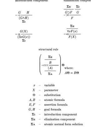
introduction component

G

H

1 \ I

-(G/\H)

~I

G(X)

3 I

-(3xG(x))

~I

structural rule

B

= C U T = = =

(A)

~A

x variable X parameter

e

substitution

elimination component

G-:JF G

: : > E -F

VxF(x)

\ I E

-F(X)

8 where:

AE>=BE>

A, B atomic formula

E, F assertion formula

G, H goal formula

~I introduction component

~E elimination component

[image:4.598.151.444.110.517.2]

~A atomic normal form solution

Figure 4.2: system

Hr.

-atomic normal form solution for the Horn language

4.2.1 Horn Formulae and Their Extensions

A feature of the Horn language, and many of the subsequent languages, is that assertion and goal subformulae have distinct syntax. For these dual syntax languages we use the syntactic variables E and F to stand for assertion formulae, and G and H for goal formulae. The syntax of Horn axioms and queries is illustrated in figure 4.3. The large prefix universal (existential) quantifiers in this figure denote the universal (existential) closure of the prefixed formula- that is, the formulae are in prenex form. Notice that although this conventional notion of Horn formulae requires prenex quantification, the deduction system

Hr.

does not.

CHAPTER 4. EXPRESSIVE POWER AND INFERENCE 67

we can prune away the input formula resulting in the simpler forms (b) and (e). For

rule based inference, (b) and (e) may be represented as the derived rules of inference

(c) and (f) respectively. The prime notation in the figure indicates that applications of

the universal elimination (\iE) and existential introduction (31) rules have replaced the bound variables of the input formula by parameters.

-AXIOM-F Ai A~ ··· A~ Ai A~ ··· A~

~

tree

w

Ai A~ · · · A~

B'

B'

B'

(a) (b) (c)

Ai A~ ··· A~ Ai A~ · · · A~

w w

Ai A~ · · · A~

G

[image:5.598.135.498.201.458.2]

-QUERY-(d) (e) (f)

Figure 4.3: inferential extensions of Horn axioms and queries

The simple correspondence between Horn formulae and derived rules of inference,

illustrated in figure 4.3, supports a proof theoretic view of a Horn problem. Read the

input formulae, not as formulae, but as rules of inference or the clauses of an inductive

definition of provable atomic formulae. This view is proposed and extended towards

more expressive languages by [Hallnas & Schraeder-Heister 90].

4.2.2

CUT

and The Quantifier Rules VE and

31

It is time to consider in detail the role played by parameters and unification in the

process of constructing solutions. The story begins here and is continued, when the

other two quantifier rules \i1 and 3E are adopted.

A solution is a composition, by application of the CUT rule, of renaming instances

of search components. Applications of \iE and 31 replace the bound variables of input formulae by parameters, so that only quantifier free atoms appear as premisses and

conclusions of components. The cut principle requires that its premiss and conclusion

is expressed by the clause:

Given the two components :E, and (A) and a substitution E> such that (AE> =BE>)

B :E2

then

(=cuT:·

)e

is a component.

(A)

:E2

The VE and :31 rules allow for any term whatever to replace a parameter. Given the two quantifier free atoms A and B we want to find a substitution (of terms for parameters) E> such that AE> and BE> are the most general syntactically identical substitution instances of A and B. That is, E> is the most general unifier (mgu) of A

and B.

Most General Unifier (mgu): The mgu E> of the two atoms A and B is a set

of equality assertions:

E> satisfies the following constraints:

Unifier: AE> and BE> are syntactically identical.

Most General: Any common substitution instance of A and B IS also a

substitution instance of AE> (BE>).

Solved Form: Each Xi is a distinct parameter that occurs in either A or B.

Each ti is a term containing parameters that occur in either A or B but

none that occur as an Xi.

The above constraints enable efficient composition of mgu's, a question considered in detail in chapter 5. The computation of an mgu given A and B has been extensively

studied since the pioneering work of [Robinson 65], see for example [Lassez et al. 88].

4.3

The Positive Edinburgh Prolog Language

CHAPTER 4. EXPRESSIVE POWER AND INFERENCE 69

4.3.1 The Or Introduction Rules VI

The sublanguage property states that just the introduction rules for the logical oper-ators appearing in the goal syntax are required for a complete normal form deduction system. Thus to extend the deduction system 1{y:, for disjunctive goals, we simply add the two or introduction rules of figure 4.4 to the existing rules.

G H

- v r - - - v r

-(GVH) (GVH)

[image:7.597.140.503.426.684.2]

~I ~I

Figure 4.4: or introduction rules (VI)

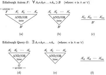
The form of the inferential extensions for the extended syntax is illustrated in figure 4.5 (a) and (d). An inferential extension still consist of a single search component. The search component still has a single atomic conclusion. However, a search component may now contain OR branches, giving rise to multiple solution components. Each solution graph of the AND/OR graphs (b) or (e) is a derived rule of inference (c) or (f), featuring a subset of the atomic premisses.

Edinburgh Axiom F:

V

A1 oA2o ... oAn :::> B (where: o is 1\ or V)

-AXIOM-p Ai A~ ··· A~

~

tree tree

B'

B'

B'

(a) (b) (c)

Edinburgh Query G:

3

A1oA2o ... oAn (where: o is 1\ or V)

Ai A~ ·· · A~ Ai A~ · · · A~

G

-QUERY-(d) (e) (f)

Figure 4.5: inferential extensions of Edinburgh axioms and queries

atomic normal form natural deduction see [Keronen 91].

4.4

The Positive Definite Language

In this section we consider the deductive machinery required for a full positive goal syn-tax. The universal quantifier introduction (VI) and implication introduction (::::n) rules are added to the Edinburgh system. This language is definite in the sense that

disjunc-tive and existentially quantified assertion formulae are not admitted. The conclusion of a rule derived from a positive definite axiom is still an atomic formula.

4.4.1

The Quantifier Introduction Rule

VI

G(X8 )

v r

-('v'xG( x))

~I

Figure 4.6: universal quantifier introduction rule (VI)

The universal quantifier introduction rule VI replaces the bound variable x in the goal VxG(x) by a parameter xs, resulting in the subgoal G(Xs), see figure 4.6. The super-script S is used to distinguish the parameter generated by application of this rule as a Skolem parameter. Unlike the parameter generated by an application of 3I, a renamed Skolem parameter

xis

is subject to the following two constraints on its use:

Skolem Constraint:

xis

is to appear literally in the solution. The mechanism to enforce this constraint is simply to treat the parameter as if it were a constant symbol, identical only to itself [Skolem 28]. That is, a Skolem parameter may only appear on the right hand side of any element Xi

=

ti of an mgu. As an

example, the mgu in figure 4.7 (a) violates this constraint.

Dependency Constraint: Xf may not appear in any assumption on which G(Xf) depends. Assumptions may be present once any of the rules

::::n,

"-'I, 3E or VE

are admitted. In general terms, enforcing the dependency constraint requires that mgu elements of the form

xi =

~s be checked to determine that the VI rule responsible for ~s occurs low enough in the solution, so that all assump-tions in which Xi occurs have been discharged. As an example, the mgu in

CHAPTER 4. EXPRESSIVE POWER AND INFERENCE 71

- - - - ' ( 1 ) p(X1) ₈

=CUT= X1 =

Yi

P(Yi8 )

-AXIOM- V I

-p(a) s

=CUT= Xl =a

p(Xf)

\:fyp(y)

-:>I (1)

p(XI):Nyp(y)

- v r - - 3 I

-Vxp(x) 3x (p(x):Ny p(y))

-QUERY- Q U E R Y

-(a) (b)

Figure 4.7: Skolem parameter constraint violations

4.4.2 The Implication Introduction Rule :JI

The deduction problem~ ?- (F:JG) is reduced by the implication introduction rule, shown in figure 4.8, to the problem~ U

{F}

?- G. That is, the antecedent F is an assumption or temporary axiom that may be used for the purpose of deriving the

conclusion G only.

[F] G

: : > I -(F:JG)

:EI

Figure 4.8: implication introduction rule (:JI)

Inferential extension may now contain assumption search components arising from the antecedents of goal implications, as illustrated in figure 4.9 (a) and (d). For each inferential extension there is a set of derived rules of inference of the form (c) or (f). The intended reading of these rules is: For each premiss Akx of the derived rule a set

of derived rules Rkx is available as assumptions. This generalization of the notion of a

rule of inference is explained in more detail in section 5.1.

Notice that the inferential extension of a formula still consists of search components with a single atomic conclusion. Hence the natural deduction formulation retains the definite character of the deduction problem. In contrast the resolution refutation proof theory is more severely affected. While any Edinburgh formula can be rewritten as a logically equivalent set of Horn clauses, once implications as goals are admitted we are outside Horn clause resolution. As an example, the axiom (F:JG):JH rewrites to the set of clauses { FV H, "'GV H}. The multiple positive literals of the resulting clauses call for a full resolution refutation strategy [Chang & Lee 73].

Positive Definite Axiom F:

-AXIOM-E A1• ···A'.

~

tre

B'.

.J

p A~l A~2 . . . A~n

~

tree

B'

(a)

VG-::;B

E A1. ···A1•

~

tree

B'.

.J

A~l A~2 ... A~,

~

~

B'

(b)

- - ( i )

Rkl

B'

(c)

A'

kl (i)

Positive Definite Query G: any formula constructed using operators 3, 'V, A, V and -::1

E A1• ···A'.

~

re

B'.

.J

G

-QUERY-(d)

E A1• ···A'.

~

re

B' .

. J

(e)

- - ( i )

Rkl

(f)

[image:10.602.142.504.95.486.2]

A'

_{kl i)}

Figure 4.9: inferential extensions of positive definite axioms and queries

available for constructing the choice point for a given goal atom now depends on its

subgoal context. Recall that this context is determined by the path from the query

to the goal atom in question. This raises the following challenges for inference engine implementations:

• A choice point cannot be completely constructed until the path to the query is known. A simple approach to this problem is to employ backward chaining search in the compose phase of the inference engine.

• Efficient logic programming engines construct choice points, as far as possible at compile time. In the presence of implications as goals, such a mechanism needs to be extended to incorporate the lookup of search components from a tree structured database at run time.

CHAPTER 4. EXPRESSIVE POWER AND INFERENCE

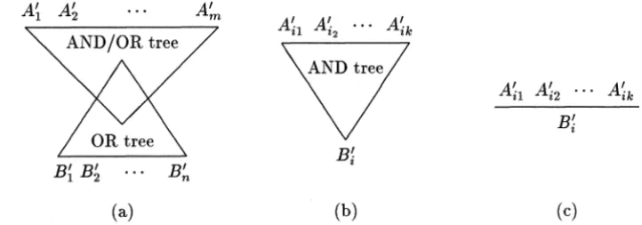
A'.Z 1 A'. Z2 · · · A'.k Z

AND tree

OR tree B' _n

(a) (b)

Ai1 Ai2 · · · Aik

B;

[image:11.598.144.505.109.235.2]

(c) Figure 4.11: components and derived rule with /\E

4.5.2 The Existential Elimination Rule

:JE

74

The existential elimination rule 3E, shown in figure 4.12, reduces an assertion 3x F(x)

to the quantifier free assertion F(X8 ). Like the VI rule, this rule generates a Skolem parameter, subject to both the Skolem and dependency constraints.

:EE

3xF(x)

3 E

-F(X8)

Figure 4.12: existential quantifier elimination rule (3E)

As we moved from the orthodox formulation of natural deduction proof (chapter 2)

to the more computational notion of a solution (chapter 3), we adopted new notation

for existential elimination. Figure 4.13 (a) illustrates the orthodox notation for an

application of existential elimination, and (b) our computational notation for the same.

The transformation from the form (a) to the form (b) can always be performed, provided

the existential elimination discharges its assumption. That is, the new notation does

not permit vacuous applications of the rule. The new notation is also more convenient

in connection with the AND/OR graph search paradigm.

Figure 4.14 displays an example solution using the orthodox notation (a) and the

computational notation (b). As a disadvantage of the new notation, the assumption

does not stand out as well here as it does in the orthodox notation. Figure 4.15

illustrates the need to carefully discharge assumptions and to check the dependency

constraint to avoid unsound inference.

The discharge of the assumption is a simple deterministic operation. To ensure

completeness one must discharge the assumption as high up in the solution graph as

possible. A simple implementation may traverse down the solution, applying

~

[F(X)] 3xF(x)

(i)

~ ~1 -3E

(F(X5 ))

3xF(x) G ~1

-3E (i)

(G) (G)

~2 ~2

[image:12.598.193.558.276.408.2]

(a) (b)

Figure 4.13: notation for existential elimination

A X I O M

-- -- -- -- -- ( 1 )

3y'tfxp(x,y)

-3E (1)

Vxp(x,Y) Vxp(x,Y;s)

- V E - - - V E

-p(Xz, YZS) s s

= C U T = (Xz = Xl )1\(Yi = yZ )

p(X,Y)

- A X I O M - - - 3I

-3y'tfxp(x,y) 3yp(X,y)

- 3E (1) - p(Xf, 3I Yi) (1)

3yp(X,y) 3yp(Xf,y)

- v r - - - I i i

Vx3yp(x,y) Vx3y p(x, y)

- Q U E R Y - - Q U E R Y

-(a) (b)

Figure 4.14: existential elimination representation example

question is encountered. A more efficient implementation would associate discharge

requirements and capabilities with parameter occurrences in solution components to

avoid the need for traversing the solution graph.

A X I O M

-'tfx3yp(x,y)

V E

-3yp(Xz,y)

-3E (1)

p(Xz, y;s) s s

= C U T = Xz =

xl '

Yi =

Y2

p(Xf, Yi)

\ i i

-'tfx p(x, Yi)

- 3I ( 1)

3y't/xp(x,y)

Q U E R Y

-Figure 4.15: dependency constraint violation

4.5.3 The Or Elimination Rule VE

The or elimination rule VE of figure 4.16 may be read as: The assertion EV F gives

rise to two possible worlds, one contains E, the other F. More generally, n binary

[image:12.598.296.440.511.627.2]

CHAPTER 4. EXPRESSIVE POWER AND INFERENCE 76

for all worlds. In the presence of disjunctive assertions, a solution for query G consists

of a set of case arguments. Each case argument establishes G for a subset of worlds.

~E

EVF

v E

-E

F

Figure 4.16: or elimination rule (VE)

For the same reasons as in the case of the :lE rule, we employ an alternative

no-tation for the compuno-tational notion of or elimination. The transformation between

applications of the orthodox natural deduction rule and our computational rule is

il-lustrated in figure 4.17. Note that natural deduction (even in normal form) permits

vacuous applications of the VE rule, but that such application cannot be expressed in

the new notation. For a different perspective on multiple conclusion rules of inference

see [Shoesmith & Smiley 78].

~

[E] [F]

_EVF

~ ~1 ~2 -vE (i)

- - - -

(E)

(F)

EVF

G G ~1 ~2

-vE - - ( i ) - - ( i )

(G) (G) (G)

~3 ~3 ~3

(a) (b)

Figure 4.17: notation for or elimination

In the presence of the VE rule, search components contain AND related atomic

con-clusions. We have now reached the most general form for search components, illustrated

in figure 4.18.

The word "AND", used above to describe the relationship between conclusion

atoms, is not totally satisfactory. It is true that a complete set of case arguments

corresponds to a solution graph of the search space when just one disjunctive assertion

occurs in the solution. There are two ways in which this model fails to reflect the

application of disjunction elimination more generally:

• Any one case argument may use only one of the disjuncts from any one solution

component instance. The example in figure 4.19 illustrates an unsound solution,

A~ A~ A' m A~l A~2 ... A~k

AND tree

A~l A~2

...

A~k

AND tree Bjl Bj2 · · · B}t B' 1 B' 2 B' n Bj1 Bj2 · · · Bj1

(a) (b) (c)

Figure 4.18: components and derived rules with VE

[image:14.600.126.513.65.753.2]

{ aVb } ?- a/\b

Figure 4.19: failure to separate cases

• A solution must contain case arguments to cover all worlds generated by disjunc-tive assertions. Figure 4.20 illustrates a failure on this count.

aVb cVd

( a/\c) -:J

f

(b/\d)-:)

f

[image:14.600.146.504.90.420.2]

?-

f

Figure 4.20: failure to cover all cases

The set of worlds to be covered by case arguments is generated as the cartesian product of sets of disjunctive conclusions. For the example of figure 4.21 there are the four worlds:

a b

c w1 w2 d w3 w4

CHAPTER 4. EXPRESSIVE POWER AND INFERENCE 78 unsound case argument in figure 4.19 used more than one disjunct from an axis of such a diagram, while the set of case arguments in figure 4.20 failed to cover the two worlds

w2 and w3.

aVb cVd

rv(al\c)

(bl\c)~f

d~f

?-

f

Figure 4.21: or elimination example

The above discussion suggests that we recognise the supervision of case arguments as a separate subtask for the inference engine. This supervisory level of the inference engine sets up the case argument context, being a set of single conclusion derived rules, and calls for a case argument search in that context.

4.6

Minimal Logic

The addition of the introduction and elimination rules for the negation operator ( rv) to the positive system results in a system for minimal logic [Johansson 36]. The elimina-tion rule for negaelimina-tion constitutes a simple definielimina-tion of the noelimina-tion of contradiction. The

subsequent use that is made of contradiction in deriving new conclusions is more con-troversial. The introduction and elimination rules for negation highlight the inadequacy of pure forward or backward chaining search strategies for compose.

(G) _{:EE :EI}

#

-~I _{rvF F}

(rvG) -~E

:EI

_#

(a) (b)

Figure 4.22: negation introduction ( rvi) and elimination ( rvE) rules

4.6.1 The Negation Rules rvi and rvE

Reductio ad Absurdum: A familiar method of argument to establish that a negation formula rvG holds is by demonstrating that a contradiction can be derived from the assumption G together with other current assumptions and axioms.

Absurdity Principle: Adherence to the semantics of classical logic demand that any formula whatsoever be derivable from a contradiction.

The reductio ad absurdum principle provides us with two points, the assumption

G and the conclusion

#,

around which to construct a solution. Let us distinguish this as a new kind of deduction problem.

Relevant Deduction Problem: Given a set of required axioms

r

and a set of

ordinary axioms~' is there a proof of G in the systemS? In symbols:

r:

~ ?-

c

s

Any solution to the deduction problem

r u

~ ?- G s

that features every member of

r

as a premiss is a solution for the corresponding relevant deduction problem.

Neither the pure backward nor forward chaining search strategy makes full use of the constraints on premisses and conclusion. Notice that this point can also be made for the implication introduction rule. The absurdity principle is discussed in the next section.

4. 7

Intuitionistic Logic

Intuitionistic deducibility requires an implementation of the absurdity principle for any goal formula, not just the negated ones. A first reading of the absurdity rule, shown in figure 4.23, might then be as a kind of introduction rule to be applied for all goal formula occurences.

#

# X

-(G) :EI

Figure 4.23: absurdity rule ( #x)

CHAPTER 4. EXPRESSIVE POWER AND INFERENCE 80

• Check the consistency of the original problem theory .6.. In the case that an inconsistency is found all queries receive an affirmative answer, until the theory

is repaired.

• Given the consistency of .6., a contradiction may still be derivable in some subgoal

or case argument contexts. For each additional assumption we call for a search

for contradiction derivable using the assumption in question. Notice that this is

another example of a relevant deduction problem.

Many (most) theorem prover implementations do not perform the first of the above

checks, preferring to assume the consistency of .6.. An example of this is the set of

support strategy for resolution refutation systems [Chang & Lee 73].

4.8

Classical Logic

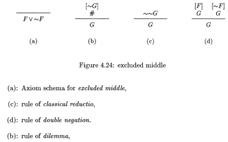
A system for classical logic results if any one of the constructs shown in figure 4.24 is

added to the intuitionistic system. These constructs are:

G G

[image:17.597.133.500.399.626.2]

(a) (b) (c) (d)

Figure 4.24: excluded middle

(a): Axiom schema for excluded middle,

(c): rule of classical reductio,

(d): rule of double negation.

(b): rule of dilemma,

In the presence of any of these alternatives the subformula property is not strictly

observed. To see this, consider the deduction problem

{} ?- (a~b)V(b~a)

There is no intuitionistic solution for this problem. The classical solution therefore

must include at least one application of the excluded middle principle, and therefore a

negated formula occurrence. No negated subformulae, however, occur in the statement

rules for moving in negations

:EE

....,a

...,H "'(E/\F)

-"-"\I -"-"\I -"-"\E

( ...,(G/\H)) ( ...,(G/\H)) ...,E ...,p

:Er :Er

:EE :EE

....,a

...,H ...,(EVF) rv(EVF)

-"'VI -"'VE -"'VE

(...,(GVH)) ...,E ...,p

:Er

:EE :EE

G ...,H ...,(E:>F) ...,(E:>F)

-~:>I -~::>E -~::>E

( ...,( G:>H)) E rvF

:Er

:EE

3x(...,G(x)) ...,(\fxF(x))

-~vr -~vE

( ...,(\fxG( x))) 3x(...,F(x))

:Er

:EE

'v'x(...,G(x)) ...,(3xF(x))

-~3I -~3E

("'(3xG(x))) 'v'x(...,F(x))

:Er

:EE

G ...,...,p

-~I -~E

("'"'G) F

:Er

rules for negative literals

(A)

:EA

(

=MX )

(A) ("'B)

:EAl :EA2 E) where:

G G AE>=BE>

x - variable

e -

substitution

A, B - atomic formula

E, F - assertion formula

...,B B

-~E---#

G, H - goal formula

[image:18.597.139.490.108.737.2]

:Er - introduction component :EE - elimination component :EA - (partial) solution

CHAPTER 4. EXPRESSIVE POWER AND INFERENCE

- - ( 1 ) - - ( 2 )

rvb b

-~E---#

# X

-- -- -- ( 1 )

b a

- ::JI--(2) : ) 1

-a:Jb b:Ja

-MX-- - v r - - - v r

-b V rvb (a:Jb)V(b:Ja) (a:Jb)V(b:Ja)

- v E - - - ( 1 )

( a:Jb )V(b:Ja)

Q U E R Y

-Figure 4.26: excluded middle example

82

The direct computational interpretation of any of the rules (b)~( d), as a kind of introduction rule for any formula whatever, suffers from serious combinatorial problems. Also, a literal implementation of alternative (a), that is the presence of all formulae of the form FVrvF as axioms, is not possible.

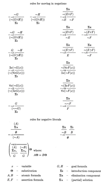
An incomplete implementation relying on recognising occurrences of complementary subgoal literals is suggested by consideration of the RGR rule of [Nilsson 80]. Well known equivalences of classical logic, enable any formula to be rewritten so that the negation operator applies only to atoms. This operation of moving in negations is

part of the process for translating formulae into clausal form for resolution. These equivalences may be included in our system as rules of inference, as shown in figure 4.25. As a result of this extension the absurdity reasoning called for by negation introduction is confined to atoms, as indicated by the special rvi rule in the figure. The special MX rule may be applied whenever two complementary, unifiable atomic goals arise in distinct case arguments.

4. 9

Alternative Languages

As seen above, classical and even intuitionistic natural deduction proof theories suffer from severe combinatorial problems. We place the blame for this on the following two features of these systems:

• The complexity of the search for contradictions. • The complexity of applying excluded middle.

[image:19.598.238.427.102.227.2]

section, cannot be expressed. Many proposed extensions of these languages, for exam-ple [Gabbay & Reyle 84], are based on intuitionistic logic, again avoiding the need for excluded middle.

Prolog has adopted the negation as failure (NAF) rule of inference [Clark 78] as the proof theoretic device for negated goals. The NAF rule of inference fits neatly, as a negation introduction rule, into a natural deduction framework. According to this rule, the deduction problem .6. ?- "'G receives an affirmative answer given that there

is a failure demonstration, denoted by :!:Fin figure 4.27, for the problem .6. ?- G.

:EF G

= N A F = = =

(""G)

Figure 4.27: negation as failure rule (NAF)

Chapter

5

Inference Engines

The search for solutions is viewed within two paradigms: • deduction employing derived rules of inference • AND/OR graph search

The derived rules of inference paradigm provides a simple conceptual model of the inference engine. AND/OR graph search, on the other hand, exposes issues relevant to efficient search. The impressive implementation technology of the logic programming language Prolog is examined. The extension of this technology to more expressive languages and full AND/OR parallel evaluation is considered.

5.1

AND/OR Graphs and Derived Rules of Inference

We began chapter 3 with a brief examination of search strategies in the context of the natural deduction rules of inference. The fact that this set of rules is systematic and fixed (for a given logic) enabled us to eliminate them, and replace each axiom and query by its inferential extension. In chapter 4 we saw that it is possible to think of the AND/OR graph, that is an inferential extension, as representing a set of derived rules of inference. Consequently, we now have two further perspectives on the search task:

Deduction employing derived rules of inference: Subgraphsofinferentialex-tensions correspond to derived rules of inference. Hence, search can be viewed in the context of reasoning within a deduction system consisting of a set of such derived rules.

AND/OR graph search: The search space for solutions consists of AND/OR graph fragments (renamed search components) connected by CUT rule

in-stances. A solution to the deduction problem at hand is a solution subgraph of the AND/OR search space.

A derived rule of inference is a generalisation of the notion of inference rule, as

presented in chapter 2. The natural deduction rules are all instances of the schema

shown in figure 5.1 (a). Such a rule leads from a set of premiss formulae {F1 ... Fn} to a single formula G as conclusion. The rule may also discharge assumption formulae

E1 ... En. In contrast, a derived rule, figure 5.1 (b), leads from a set of premiss formulae {A1 ... An} to a set of conclusion formulae {B1 ... Bm}· The set of conclusions being read disjunctively. Further, the assumptions that may be discharged are not formulae

but sets of derived rules R1 ... Rn.

- - ( i ) - - ( i ) - - ( i ) - - ( i )

E1

En

R1

Rn

F1

Fn

A1

An

(i) (i)

G Bl··· Bm

[image:22.597.213.450.264.355.2]

(a) (b)

Figure 5.1: inference rule schemas

The set of derived rules produced by extend depends on the particular deduction problem statement at hand. Further, as the search proceeds, the set of available rules

varies depending on subgoal and case argument context. The best we can do, a priori,

is to distinguish the three subclasses of derived rules illustrated in figure 5.2. Rules

drawn from each of these subclasses occupies a distinct niche in a complete solution:

- - ( i ) - - ( i ) - - ( i ) - - ( i )

R1

Rn

R1

Rn

A1

An

(i) A1

An

(i)

B1··· Bm B1··· Bm

(a) (b) (c)

Figure 5.2: subclasses of derived rules

(a): A query rule has an empty conclusion, and is derived from the query formula.

All paths in a solution are terminated at the bottom by a query rule instance.

(b): A proper rule is derived from an axiom or query that contains implications or

negations as assertion subformulae.

(c): A fact rule has an empty set of premisses, and may be derived from an axiom

or query. All paths of a solution are terminated at the top by a fact rule

CHAPTER 5. INFERENCE ENGINES 86

Deduction systems, such as the above, that include extended forms of inference rules have received some attention recently. [Shoesmith & Smiley 78] investigate the exten-sion to rules with multiple concluexten-sions. [Schraeder-Heister 84] argues that rules that discharge other rules as assumptions are a "natural extension of natural deduction".

The account of implementation techniques in this chapter relies on both the derived rules and AND/OR graph search paradigms. The AND/OR graph view is strong for many issues in search and representation. The derived rule view comes into its own when we wish to present a simple user view of the inference engine, see chapter 6.

5.2

Search as a Constraint Satisfaction Problem

We take the definition of ANF solution graph of section 3.4.2 as a starting point for

the exploration of implementation issues. That definition consisted of the following five constraints on the form of a solution graph:

• Query Relevance • Axiom Relevance • Resolved Choice

• Substitution Consistency • Loop Freeness

As a first step towards computational realization we read this definition as a constraint satisfaction problem. The remainder of this chapter deals with the problem of applying these constraints constructively to the task of finding solutions.

Traditionally inference engines apply either forward chaining (axiom relevance) or backward chaining (query relevance) elaborating a single partial solution at a time (resolved choice) while maintaining full substitution consistency for the current partial solution. The loop freeness constraint is often ignored. The Prolog inference engine, to be described a little later, conforms to these conventions, and provides us with a good point of reference. The following subsections examine the five constraints in more detail.

5.2.1 Axiom and Query Relevance

• As illustrated in section 3.2, the query relevance constraint is built into backward chaining strategies. Only those subgraphs of the search space containing the query are explored.

• In cases where the search space is too large to permit exhaustive, uninformed search, the generic backward chaining scheme can be specialised to incorporate control knowledge. Backward chaining is conceptualised as simple goal reduction with choice of subgoal and rule. This point is expanded in section 6.2.

• Backward chaining simplifies some implementation issues. For example the con-struction of complete choice points is possible, as the path to the query is always known. Implementation techniques developed in the logic programming context may be applied.

Backward chaining does not apply the axiom relevance constraint to limit search. This problem is painfully obvious in the case of relevant deduction problems when the conclusion is a contradiction, as is the case with reductio ad absurdum. Haridi [Haridi 81] suggests that forward chaining should be adopted for these kinds of sub-problems. Note, however, that a forward chaining strategy does not make effective use of query relevance. What is called for is a search regime that is sensitive to all avail-able constraints. A first step in this direction would seem to be to apply the relatively expensive substitution consistency constraint incrementally. For some suggestions in this direction see the work [Sickel 76] on clause interconnection graphs.

5.2.2 Resolved Choice

A spectrum of search strategies from depth first to breadth first is characterized by the number of partial solutions maintained at any one time. Common practice is to simplify implementation and maintain resolved choice by choosing the extreme depth first end of the spectrum. The full breadth first strategy, at the other extreme, is often impractical on combinatorial grounds. In section 5.5.3 we consider the implementation of strategies in the middle ground, enabling the concurrent exploration of a number of promising partial solutions. The following paragraphs set the scene in the context of backward chaining search strategies.

CHAPTER 5. INFERENCE ENGINES 88

Subgoal Choice: Select a subset of the subgoals for expansion from the current set of partial solutions. In other words, given a set of partial solutions, select a set of choice points. For sequential, one solution at a time implementations both of these sets are singletons.

Rule Choice: Given a subgoal, select the derived rules to be applied from the set of candidate rules. In other words, given a choice point, select a set of CUT

rule instances.

The above conceptual model of the choices faced by a search algorithm is commonly found in accounts of the Prolog language. Prolog relies on the programmer to exploit his understanding of a fixed choice algorithm to control the search process. In section 6.2, encouraged by the success of this approach, we explore an alternative control paradigm based on the same conceptual model.

5.2.3 Substitution Consistency

A simple extension of the composition of substitutions operation of [van Vaalen 75]

replaces a set of mgu's in solved form (see section 4.2.2) {81, 82, ... , 8m} with a single mgu in solved form 8, such that for any term t

Composition of MGUs: Given a set of mgu's {81, 82, ... , 8m} in solved form the following algorithm finds their composition if one exists and otherwise halts with fail status.

step 1: Let 8 be 81 U 82 U ... U 8m. That is 8 is a set of equality assertions

{X1

=

t1, X2

=

t2, ... , Xn

=

tn}·

In order to reduce 8 into solved form repeat step 2 until no longer applicable.

step 2: Choose any pair of equality assertions (Xi

=

ti) and (Xj

=

tj), such that the two parameters Xi and Xj are identical. If the two terms ti and

tj unify then replace the two assertions in 8 by the set of assertions that is the mgu of ti and tj, otherwise halt with failure status.

Return 8 as the answer.

be postponed. These freedoms are often not exploited by implementors to improve

performance. Composition of unifiers is typically the most expensive operation of an

inference engine implementation.

As discussed in chapter 4, the quantifier rules VI and :3E impose two further con-straints on substitutions:

Skolem Constraint: This condition can be maintained by restricting Skolem

param-eters to appear only on the right hand side of mgu equality assertions.

Dependency Constraint: To maintain this condition it is necessary to check that

any VI rule occurrences do not rely on undischarged assumptions. A very simple implementation can check the well formedness of a complete candidate

solution.

5.2.4 Loop Freeness

The normal form for natural deduction proofs constrains the form of subproof for major

premisses of elimination rules only. This leaves the door open for paths through minor

premisses containing multiple occurrences of the same subproblem. In the case of a "no

assumptions" language like Prolog a subgoal that is identical or subsumes a subgoal

lower down on the path to the query signals the presence of a loop. In the case that

assumptions are present, a sufficient additional condition for a loop is that the upper

subproblem not have more premisses available to it than does the lower one.

-AXIOM-F F-::JE

: : > E

-

-AXIOM-E-::JF

E

=CUT=

E

: : > E -F

[image:26.598.149.470.496.621.2]

(a)

Figure 5.3: proof loops

-AXIOM-""F F

-~E---#

=CUT=

#

# X

-F

(b)

The potential for loops exists when occurrences of the elimination rules with minor

premisses, that is ::JE and "-'E are present. Figure 5.3 illustrates the simplest loop

elements. Notice that in the case of "-'E, the absurdity rule #X is also involved. The

first step in minimizing the cost of loop detection is to perform a loop check only when

CHAPTER 5. INFERENCE ENGINES 90

5.3

Implementation Technology

The purpose of this section is to establish a point of reference for inference engine

imple-mentation technology. Programs for solving deduction problems have been developed

in a number of distinct settings:

• Resolution refutation theorem provers.

• Question answering systems for deductive databases.

• Logic programming language implementations.

• Expert systems inference engines.

• Verification of the correctness of programs and hardware designs.

Despite the various demands of the intended area of application, many current

systems are based on a set of common elements:

• Backward chaining search is used to maintain query relevance. Some systems

incorporate a carefully limited forward chaining preprocessor.

• A single partial solution is explored at any one time, with backtracking on failure

or depth bound. An important exception is the processing of ground atoms by

database operations.

• Substitution consistency is maintained by a unification algorithm together with

clever representation schemes for terms instantiated by unification. Substitution

consistency is fully maintained for the single current partial solution.

Conforming to the above model, the logic programming community has largely

focused its attention on the development of implementation techniques for the Horn

language. First, recall that Horn clauses are mapped into Horn rules by extend.

Sec-ond, recall that case arguments are derivations consisting of instances of Horn rules

only. These two relationships suggest that we adopt this work as a point of

refer-ence. The remaining sections of this chapter explore implementation issues from this

perspective.

5.3.1 The Prolog Inference Engine

The following paragraphs point out the key elements of current logic programming

sys-tems implementations. We focus on the structure sharing implementation technology

developed for the Prolog language. This section deals with the the pure Horn

of implementation techniques for more expressive languages. For more comprehensive

descriptions of current techniques see for example [A1t-Kaci 90], [Bruynooghe 82) and

[Campbell 84].

Prolog exploits the reading of sets of formulae as programming language procedure

definitions. This procedural semantics of Prolog determines that the AND/OR search

space be explored sequentially in left to right and depth first order. The stack based

representation of computation state, developed for procedural programming language

implementations, is used.

As an illustration, the partial solution of figure 5.4 (a) is represented by the data

structures in (b). These data structures can be divided into a static and dynamic

component:

Structure Store: The static structure of the Horn rules is kept here.

Stack: The structure and substitutions for the current (partial) solution are main-tained as a sequence of stack frames.

The current (partial) solution tree is mapped onto the stack in chronological order.

There is one stack frame for each occurrence of a Horn rule instance in the solution

being represented. A stack frame consists of a pointer to the Horn rule structure, a

pointer to a "parent" stack frame, a vector of bindings, as well as other information left

out of the figure for clarity. The vector of bindings contains one entry for each distinct

parameter occurring in the rule. The result of applying this vector as a substitution to

the rule structure is the desired rule instance.

Each binding, an equality assertion of the form Xi

=

t, is represented by a binding

vector entry. The renaming i is implicit in the context of the binding as part of a

stack frame. The name X is associated with the vector offset. The term tis explicitly

represented as a pair of pointers, one pointing to the term structure, the other to the

stack frame where bindings for parameters occurring in the term structure are to be

found.

The fact that only a single partial solution is represented at any one time implies

that just a single set of bindings, being the composition of unifiers for the current partial

solution, is required. The composition of unifiers is represented by the entire set of

non-null bindings on the stack. In the case of the example of figure 5.4, the composition of

the three unifiers 81, 82 and 83 is represented by four binding vectors.

The above representation of the composition of unifiers has more structure than our

textual representation as a set of equality assertions. The binding pointers form a graph

consisting of a set of connected components. Each connected component corresponds

CHAPTER 5. INFERENCE ENGINES

Rl:

le

T

1

A1 1

R4: · -B4

le

T

3

A1 2 B1 (a) -

4-structure

-I--parent

vector of

bindings

structure

---r- parent

vector of

bindings

structure

--parent

vector of

bindings

structure

--parent

vector of

bindings

[image:29.600.165.475.91.422.2]

(b)

Figure 5.4: stack data structure for single solution

92

two components. That is, the Prolog unifier applies the well known UNION-FIND algorithm (see for example [Aho, Hopcroft & Ullman 74] for a description of union-find). For future reference note that the unifier is free to apply the path compression optimization of UNION-FIND.

Figure 5.4 is a simplification. The structure of the current partial solution is repre-sented, while the information required for conducting the search is left out. This infor-mation consists of choice points and a trail. Two kinds of choice points are recorded on the stack:

Rule Choice: This corresponds to the CUT choice point of our AND/OR graph model. Just a single pointer is needed to step through the sequence of rules. Subgoal Choice: The antecedent of a Horn clause is a flat sequence of atoms.

A single pointer is again sufficient to maintain the state of the left to right traversal of this sequence.

The trail is a chronological record of binding operations, consulted when undoing bind-ings on backtracking. The trail also fits in with the stack discipline.

choice points, together with clever indexing schemes, contribute to the efficiency of Prolog implementations.

5.4

Extended Logic Programming

A logic programming language consists of two sublanguages, as recommended by the slogan

Algorithm = Logic

+

Control

of [Kowalski 79a). We shall refer to these two component languages as the problem language and the control language. In this section we consider the prospect of extending the expressive power of these two languages as well as the issue of exploiting parallel hardware for solving deduction problems.

Let us first look at current proposals for extending the Prolog inference engine to deal with larger subsets of the full first order language as the problem language. It is instructive to consider goal and assertion syntax separately:

Goal Syntax: [Gabbay & Reyle 84) and [Bollen 88) have demonstrated implementa-tions incorporating the implication introduction rule. Implementaimplementa-tions of the full positive goal syntax, based on the transformations of [Lloyd & Topor 84), also exist [Thorn

&

Zobel 88). Even negated goals, implemented by the negation as failure mechanism, may be regarded as intuitionistic negation with respect to a completed program [Clark 78), [Shepherdson 88).

Assertion Syntax: Recall that the only operators admitted by the Prolog assertion syntax are '>/ and ::). The author knows of no implementations that extend the inference engine to deal directly with enriched assertion syntax. Several meta interpreters have been proposed for asserted disjunctions and negations, see for example [Smith & Loveland 88).

In terms of the language hierarchy of chapter 4, direct implementations have not reached beyond the positive definite language

P.

We suggest that the reason why logic programming systems do not offer the expressive power of the full assertion syntax are at least threefold:

CHAPTER 5. INFERENCE ENGINES

94

Negation As Failure: Both disjunctive and existentially quantified assertions tend to "block" negation as failure results. The semantics of a language incorpo-rating these constructs is not clear.

Proof Theory: No resolution refutation proof theories are known for languages intermediate between the Horn language and full first order classical logic. The natural deduction formulation now informs us what proofs in these languages look like.

Concerning the expressive power of the control language: The procedural semantics of Prolog determine a backward chaining, depth first, single solution search strategy. The knowledgeable programmer escapes these restrictions using meta programming techniques. That is, the control language is expressively inadequate for many applica-tion areas. Again, the procedural semantics blocks extension of expressive power.

Recently, the exploitation of parallel computing hardware has become a major fo-cus for logic programming research, see for instance [Gregory 87], [Kacsuk 90] and [Wise 86]. The procedural semantics of Prolog enable the efficient implementation of the language on sequential machines. While some parallelism is available within this model, a fuller exploitation of parallelism cannot tolerate a sequential execution model. Perhaps it is obvious by now that we propose an approach to logic programming, that does not rely on the procedural reading of formulae. Our aim is to unblock the development of more expressive languages and implementations that can exploit full AND/OR parallelism. The prospect of an efficient inference engine based on the AND/OR graph paradigm is explored in the next section. Top level language design issues are taken up in the next chapter.

5.5

Implementation Techniques for Extended Languages

The following subsections present refinements of the Prolog data structure to support implementation of more expressive and parallel languages. The AND /OR graph repre-sentation for solutions and search spaces suggests data structures for implementation of extended languages.

5.5.1 More Expressive Sequential Languages

stack based scheme, with each stack frame representing a derived rule of inference, for

the more expressive languages?

The generalisation of the implementation to the Edinburgh language is very simple.

The only point of change concernes the subgoal choice pointer. For a Horn rule this

pointer traverses left to right through a sequence of atoms. For the Edinburgh language

this is generalised to a left to right, depth first enumeration of the solution trees of an

AND /OR tree with atoms as leaves.

The next step up in complexity of inferential extensions is the presence of

assump-tion search components. Recall that assumpassump-tion components are generated by

impli-cations and logical negations as goals (the

:::)I

and rvi rules of inference), present in the

positive definite language. The set of inferential extensions available for the

construc-tion of a soluconstruc-tion to a subproblem depends now on the context in which the subproblem

occurs.

The necessary extension of data structures is illustrated in figure 5.5. A context

pointer is allocated in each stack frame. A context being a set of assumption search

components, each sharing some of their bindings with the stack frame that created the

assumption. The representation of an assumption component in the structure store

includes a list of common parameters the component shares with other components of

the inferential extension. This information is needed to initialize binding vectors for

the component's stack frame. Contexts are stored in a tree structured data base.

structure

r - parent

context

vector of bindings

f---+-structure store

tree structured database of assumptions

Figure 5.5: extended stack data structure

The most general form of search component contains an AND/OR tree of

conclu-sions, as well as premisses. A stack based inference engine can still be used to construct

[image:32.595.254.419.464.672.2]

CHAPTER 5. INFERENCE ENGINES 96

sequence of calls to the inference engine, each resulting in either a case argument being

returned or in failure.

The data structure illustrated in figure 5.5 is adequate for representing a case

ar-gument. The context mechanism, however, needs to be extended to provide a wider

range of services. A non-empty initial context may be supplied to the inference engine

to direct the search for a case argument. As well as a context of assumptions, a case

argument is associated with an "anti-context" of assumptions. The anti-context is the

set of assumptions not available in the world of the case argument.

5.5.2

Single Solution AND Parallelism

While appropriate for sequential implementations, a stack based representation cannot

be maintained when a set of asynchronous processes co-operate to build up a solution.

If we abandon the stack discipline, we arrive at the data structure displayed in figure 5.6. This data structure is a graph, maintained in a heap store, perhaps distributed

across a number of processors. This AND graph data structure is also appropriate

for implementations designed to avoid unnecessary recomputation of subgoals on

back-tracking.

R3: -B3

Rl:

lo

T

=2

le

T

1 A1

1

R4:

-·-B4

le

T

3 A1

2

B1

(a)

vector of bindings

R3

I

vector of

bindings vector of bindings

R2 R4

I

I

vector of bindings

Rl

[image:33.597.171.467.426.634.2]

(b)

Figure 5.6: AND data structure for single solution

Notice that this data structure still represents just a single (partial) solution, and

therefore can only support single solution AND parallelism. It is common in the

liter-ature to distinquish two forms of single solution AND parallelism:

Stream AND Parallelism: This form occurs when concurrent subgoals share

variables.

The distinction shows up in our AND graph model in two ways: Firstly, concurrent

access to shared bindings must be controlled to maintain the integrity of the

compo-sition of unifiers operation. Secondly, a bindings dependency analysis is required to

determine the consequences of a failure on concurrent subgoals. For a more detailed

discussion of AND parallelism see [Gregory 87].

5.5.3 Multiple Solutions

AND/OR

Parallelism

A further refinement of the data structure is required to represent multiple solutions.

Let us suppose that the premisses Ai and A~, of the example in the preceding

sec-tion, also unify with R5 and R6, as shown in figure 5.7 (a). Depending on the success

of the composition of unifiers operation, there are from zero to four well formed

par-tial solutions here. The data structure, shown in (b), represents the four candidate

solutions.

The reader may have noticed already that, unlike in the simple motivational

pre-sentation of chapter 1, bindings are not associated with unifiers but with derived rule

occurrences. The advantage of the current scheme is that the binding for any specified

parameter is readily located at a fixed vector offset.

When multiple partial solutions are represented, a number of binding vectors may

be associated with a single derived rule occurrence. That is, a rule occurrence in this

data structure may stand for a number of distinct substitution instances of the rule.

The data structure of figure 5. 7 stands for a set of candidate solutions. We need a

second level representation to pick out the well formed (substitution consistent and loop

free) solutions from among these candidates. The representation we propose here is a

refinement of the ATMS labelling scheme introduced in chapter 1. The graph structure

of a solution is represented explicitly by a label, while the composition of substitutions

is not, as explained below.

The graph structure of a solution is uniquely determined by its set of binding vectors.

Further, only the ambiguity of multiple binding vectors for the one subgoal needs to

be resolved. For the example of figure 5.7, the structures of the candidate solutions

are picked out by the labels shown in figure 5.8. Only labels corresponding to the well

formed (partial) solutions are to be kept. Any label for a (partial) solution containing

an inconsistent set of bindings or a loop (a nogood) is removed. Search effort should

not be wasted on those portions of the AND/ 0 R data structure that do not appear in

any label. Many implementations would garbage collect such structures.

CHAPTER 5. INFERENCE ENGINES

R3:-B3

lo

T

=z

R4:

-B4

Al

R l :

-(a)

T3· vector of

bindings

R3

T2:

I

T5:

vector of T7: vector of

bindings vector of bindings bindings

R2 R5 R4

Tl:

I

T6:

I

T4:

I

vector of

bindings

vector of

bindings

vector of

bindings

Rl

(b)

T9: vector of

bindings

R6 T8:

I

vector of

[image:35.600.199.453.90.510.2]

bindings

Figure 5.7: AND/OR data structure for multiple solutions

{'l'l, 1:'4} {'l'l, 1:'8} {1:'6, 1:'4} {1:'6, 1:'8}

Figure 5.8: labels

98

as the composition of substitutions in solved form, since a number of bindings may

exist for the one parameter. Also, the path compression optimization cannot always

be applied. Two options for implementing the composition of substitutions are:

• Call on the unifier to determine the composed binding for a parameter

dynami-cally. In this case, the degree to which the set of bindings approximates solved

• Maintain an explicit representation of the composition with the label. This may

well be feasible when restricted to a critical subset of parameters.

The above description of AND/OR parallel evaluation omits discussing mechanisms

to support backtracking search. The reason for this omission is that the author's

exper-imental implementation work has focussed on the non-backtracking language described

in the introduction. It has also assumed that only Horn rules are present. A compre-hensive description of feasible implementation techniques for more expressive parallel

Chapter 6

Exploiting the Representation

A natural deduction solution can be readily understood as an argument leading from

a set of axioms, by way of simple principles of deduction, to the query. Atomic normal

form extends this explanative power of natural deduction. The very detailed steps of

reasoning are replaced by derived rules of inference, each justified by a particular input

formula. This perspicuous representation can be exploited as follows:

• As a graphic display, it may be used for purposes of explanation, testing and

debugging.

• Reflected as a theory accessible to introspection, it may be used for purposes of

control and to meet other practical demands placed on the reasoner.

6.1

Visualization

Having presented a mechanical reasoner with a deduction problem ~ ? - G and a finite amount of time for computation, we expect to receive as the answer a set (possibly

empty) of proofs, together with an indication of whether this set contains all the proofs

there are. Each of the proofs is to be a solution for the given deduction problem, that

is they are proofs of

r r

G (where:

r

~ ~).

In this setting, we can think of a proof as explaining which subset of the axioms, and

by what methods of reasoning, lead to the conclusion G. The following two subsections treat explanation in this sense only. The aim is to display a solution in such a way

that it can readily be grasped as an explanation. The third subsection extends this

treatment to the display of partial solutions, for the purposes of testing and debugging.

The aim being to observe the progress being made in covering the search space.