Simulation and optimisation in ion chromatography

Simulation and Optimisation in Ion

Chromatography

Boon Khing Ng

Bachelor of Science (Hons)

A thesis submitted in fulfilment of the requirements for the degree of

Doctor of Philosophy

Declaration

To the best of my knowledge, this thesis contains no copy or paraphrase of material previously published or written by another person, except where due

reference is made in the text of the thesis

Boon Khing Ng

22nd _{July, 2011}

This thesis may be available for loan and limited copying in accordance with the Copyright Act 1968

Boon Khing Ng

Acknowledgement

A/Prof Robert Shellie, A/Prof Greg Dicinoski and Prof Paul Haddad for being awesome supervisors, especially for all your precious guidance, advice as well as financial support.

Members of ACROSS group for being great people during my candidature.

Financial support in the form of scholarships and sponsorships from Australian Research Council and Dionex Corporation are gratefully

acknowledged.

Statement of Co-Authorship

The following people and institutions contributed to the publication of the work undertaken as part of this thesis:

[1] Robert A. Shellie (20%), Boon K. Ng (35%), Greg W. Dicinoski (15%), Samuel D. H. Poynter (10%), John W. O'Reilly (4%), Christopher A. Pohl (1%), Paul R. Haddad (15%)

Details of the Authors roles:

Boon K. Ng executed the laboratory tasks, computational programming and simulation

Robert A. Shellie, Boon K. Ng and Paul R. Haddad wrote the draft manuscript Robert A. Shellie, Boon K. Ng, Greg W. Dicinoski, Samuel D. H. Poynter and Paul R. Haddad contributed to the algorithm proposal and development

Robert A. Shellie, Boon K. Ng, Greg W. Dicinoski and Paul R. Haddad assisted with publication refinement and presentation

John W. O'Reilly set up the data library prior to this research study Christopher A. Pohl established the need of study and provided valuable feedback on the work

[2] Philip Zakaria (50%), Greg W. Dicinoski (25%), Boon K. Ng (4%), Robert A. Shellie (4%), Melissa Hanna-Brown (2%), Paul R. Haddad (15%) Details of the Authors roles:

Philip Zakaria executed the laboratory tasks, computational programming, simulation and wrote the draft manuscript

Philip Zakaria, Greg W. Dicinoski, Boon K. Ng, Robert A. Shellie and Paul R. Haddad contributed to the algorithm proposal and development

Philip Zakaria, Greg W. Dicinoski and Paul R. Haddad assisted with publication refinement and presentation

Melissa Hanna-Brown established the need of study and provided valuable feedback on the work

[3] Boon K. Ng (35%), Robert A. Shellie (20%), Greg W. Dicinoski (15%), Carrie Bloomfield (10%), Yan Liu (4%), Christopher A. Pohl (1%), Paul R. Haddad (15%)

Boon K. Ng and Yan Liu executed the data acquisition Boon K. Ng and Robert A. Shellie wrote the draft manuscript

Boon K. Ng, Robert A. Shellie, Greg W. Dicinoski, Carrie Bloomfield and Paul R. Haddad contributed to the method translation and development

Boon K. Ng, Robert A. Shellie, Greg W. Dicinoski and Paul R. Haddad assisted with publication refinement and presentation

Christopher A. Pohl established the need of study and provided valuable feedback on the work

[4] Viktor Drgan (20%), Boon K. Ng (20%), Marjana Novič (10%), Greg W. Dicinoski (10%), Milko Novič (10%), Robert A. Shellie (10%), Paul R. Haddad (15%)

Details of the Authors roles:

Viktor Drgan performed the computational programming and simulation Boon K. Ng and Viktor Drgan executed the data acquisition

Viktor Drgan, Paul R. Haddad and Boon K. Ng wrote the draft manuscript Viktor Drgan, Boon K. Ng, Marjana Novič, Greg W. Dicinoski, Milko Novič, Robert A. Shellie, Paul R. Haddad contributed to the proposal of algorithm and development

Viktor Drgan, Boon K. Ng, Marjana Novič, Greg W. Dicinoski, Milko Novič, Robert A. Shellie, Paul R. Haddad assisted with publication refinement and presentation

We the undersigned agree with the above stated “proportion of work undertaken” for each of the above published (or submitted) peer-reviewed manuscripts contributing to this thesis:

Signed: __________________ ______________________ A/Prof Greg W. Dicinoski Prof Emily F. Hilder

Supervisor Graduate Research Coordinator

List of Publications

Description Number of Publications National International

Research Papers 4

Oral Presentations 1 3

Poster Presentations 2 3

Refereed Journal Articles

[1] Robert A. Shellie, Boon K. Ng, Greg W. Dicinoski, Samuel D. H. Poynter, John W. O'Reilly, Christopher A. Pohl, Paul R. Haddad. Prediction of analyte retention for ion chromatography separations performed using elution profiles comprising multiple isocratic and gradient steps. Anal. Chem. (2008), 80(7), 2474-82. (Chapter 4)

[2] Philip Zakaria, Greg W. Dicinoski, Boon K. Ng, Robert A. Shellie, Melissa Hanna-Brown, Paul R. Haddad. Application of retention modelling to the

simulation of separation of organic anions in suppressed ion chromatography. J. Chromatogr. A (2009), 1216(38), 6600-10. (Chapter 4)

[3] Boon K. Ng, Robert A. Shellie, Greg W. Dicinoski, Carrie Bloomfield, Yan Liu, Christopher A. Pohl, Paul R. Haddad. Methodology for porting retention prediction data from conventional-scale to miniaturised ion chromatography systems. J. Chromatogr. A (2011), 1218, 5512-19 (Chapter 6)

Conference Presentations

[1] Boon K. Ng, Greg W. Dicinoski, Robert A. Shellie, Samuel D. H. Poynter, John W. O'Reilly, Christopher A. Pohl, Paul R. Haddad. Ion chromatography in-silico. Poster presented by Boon K. Ng at the Royal Australian Chemical Institute 14th Research and Development Topics Conference 2006 (RACI 14th R&D Topics Conference 2006), Wollongong, Australia, 5 – 9 December 2006

[2] Boon K. Ng, Greg W. Dicinoski, Robert A. Shellie, Christopher A. Pohl, Paul R. Haddad. in-silico Simulation of Retention in Ion Chromatography Using Multi-Step Gradient Eluent Profiles. Poster presented by Boon K. Ng at the ACROSS Symposium on Advances in Separation Science 2008 (ASASS 2008), Hobart, Australia, 8 – 10 December 2008

[3] Boon K. Ng, Robert A. Shellie, Greg W. Dicinoski, Christopher A. Pohl, Paul R. Haddad. Porting Retention Data from Conventional to Microbore Ion Chromatographic Systems. Lecture presented by Boon K. Ng at the RACI 17th

R&D Topics Conference 2009, Gold Coast, Australia, 6 – 9 December 2009

[4] Boon K. Ng, Robert A. Shellie, Greg W. Dicinoski, Christopher A. Pohl, Paul R. Haddad. Porting Retention Data from Conventional to Microbore Ion Chromatographic Systems. Lecture presented by Boon K. Ng at the Pittcon Conference and Exposition 2010 (Pittcon 2010), Orlando, Florida, USA, 28 Feb – 5 March 2010

[5] Boon K. Ng, Greg W. Dicinoski, Robert A. Shellie, Christopher A. Pohl, Paul R. Haddad. Real Time in-silico Simulation of Retention under Multi-step Gradient Elution Conditions in Ion Chromatography. Poster presented by Boon K. Ng at the Pittcon 2010, Orlando, Florida, USA, 28 Feb – 5 March 2010

[6] Greg W. Dicinoski, Philip J. Zakaria, Paul R. Haddad, Boon K. Ng, Robert A. Shellie, Melissa Hanna-Brown, Roman Szucs. Computer-based Simulation and Optimisation of Ion Chromatographic Separations of Pharmaceutically

Related Compounds. Poster presented by Greg W. Dicinoski at the Pittcon 2010, Orlando, Florida, USA, 28 Feb – 5 March 2010

Invited Conference Presentation

[1] Paul R. Haddad, Greg W. Dicinoski, Robert A. Shellie, Boon K. Ng, Samuel D. H. Poynter, Computer Simulation and Optimisation of Separations in Suppressed Ion Chromatography Using Combined Isocratic and Gradient Elution Profiles. Lecture presented by Paul R Haddad at the Pittcon 2008, New Orleans, Louisiana, USA, 2 – 7 March 2008

a degree of interaction between the analyte and stationary phase

Am amount of analyte present in mobile phase

As amount of analyte present in stationary phase

b effective charge of the analyte relative to competing ion

B gradient ramp (mM/min)

DA distribution coefficient of the analyte between mobile and

stationary phases

E- _{competing ion}

Ey- competing ion carries charge of y

competing ion carries charge of y in mobile phase total amount of eluent in the column segment z after v movement of mobile phase through the column

total amount of the analyte i in the column segment z after v movement of the mobile phase through the column

function f dependent on the eluent concentration in mobile phase of the column segment z after m movements of the mobile phase

G compression factor in gradient condition

H plate height of the analyte

IC ion chromatography

i.d. internal diameter

k retention factor of the analyte

kf retention factor of the analyte at the elution concentration

KA,E ion-exchange selectivity coefficient between the analyte and

the eluent competing ion

L column length (cm)

Lfinal total distance travelled of the analyte in the step (cm)

m cubic coefficient of the numerical incremental isocratic steps model

m parameter obtained from linear regression for Drgan et al. peak width model[1]

M+ insoluble matrix material comprising a fixed positive charge min Rs minimum resolution

n quadratic coefficient of the numerical incremental isocratic steps model

n parameter obtained from linear regression for Drgan et al. peak width model[1]

N number of plates of the analyte during isocratic elution o linear coefficient of the numerical incremental isocratic

steps model

Q effective ion-exchange capacity of the stationary phase

r normalised resolution product

R gradient ramp (mM/mL)

Rs resolution

t Students t-test

tapp total apparent time available for movement in the step

tf final fraction of retention which will be less than or equal to

0.05 min

tlag time taken of the new step to reach the analyte (min)

tm void time of the mobile phase to fully fill the column (min)

tm(step) void time of the mobile phase in relation to the step time

tnew updated void time based on the length remaining of the

analyte

tstep step time (min)

tR retention time of the analyte (min)

t’R adjusted retention time of the analyte (min)

tRi isocratic retention time observed under isocratic conditions

at gradient initial concentration (min) u flow-rate of the eluent (mL/min)

vinitial initial velocity of the analyte in gradient elution (cm/min)

Vm void volume of the mobile phase inside the column (mL)

VR retention volume of the analyte (mL)

V’R adjusted retention volume of the analyte (mL)

Vz volume of the connecting tubing between the outlet of the

gradient-generating device and the top of the column

w peak width of the analyte

wave average width of the two adjacent peaks

x charge of the analyte

y charge of competing ion

σ variance of the peak width

ΠRs product of resolution

Mathematical Equation Equation _NumberPage

Am⇌ As 1.1 1

1.2 1

1.3 2

⇌ 1.4 2

⇌ 1.5 2

1.6 2 1.7 11 1.8 12 1.9 12 1.10 14 1.11 14 1.12 14

[ ]

[ ]

[ ] [ ]

[ ] [ ]

s y -x m x -y m y -x s E A, E A E A = K n 3 2 1

i = x + x + x +....+ x

V

1.13 16

1.14 16

1.15 17

1.16 18

1.17 20

1.18 20

1.19 20

1.20 20

1.21 21

1.23 22

1.24 24

1.25 24

1.26 25

3.1 43

4.1 57

4.2 63

4.3 64

4.4 64

4.5 64

4.6 68

R log b -a = k log

L = H σ2

u D 2 =

H A

i

R R R

t t N t 4 = w

∑

1 = i stepi R

R =t + t

2 step 1 step R

R = t +t +t

t _{n 4.7 68}

4.8 73

4.9 74

4.10 74

( )

[ ]

(

)

i - _+Bt

E a

L =

t v

4.11 74

4.12 74

4.13 74

4.14 75

m moved lag _L t

L =

t 4.15 75

4.16 75

4.18 76

5.1 89

5.2 89

5.3 94

j j = vt

L _{5.4 94}

v L =

t R

f 5.5 94

∑

1 = j j m

f

R = t + t + t

t _{5.6 96}

Abstract

Ion chromatography (IC) is the premier technique for the separation of inorganic and organic ions. Two fundamental elution regimes, namely isocratic and

gradient elution, are available for separation but both are often inadequate for the separation of complex mixtures. Hence, complex elution profiles involving multiple isocratic and linear gradient steps have become the most attractive solution to accomplish the desired separations. However, the number of parameters requiring trial-and-error optimisation of such elution profiles demands a huge investment in time. This problem can be solved through the development of in-silico (computerised) simulation, and ultimately optimisation, methods.

The Virtual Column Separation Simulator (Dionex Corporation, Sunnyvale, CA, USA) is an efficient commercial software package for simulating and

optimising IC separations. However, it has a number of limitations. The objective of this study was to address the limitations of the Virtual Column Separation Simulator and improve its prediction and optimisation abilities. This project focussed on improving the algorithms used for simulation and modelling of retention and peak width.

retention times under complex eluent profiles using these methods relied on monitoring the analyte displacement through the chromatographic column. The three devised algorithms mapped the position of the analyte in different ways where the position mapping methods of the three algorithms relied on

mathematical iteration (which this algorithm was entitled the “linear analyte displacement model”), integrated displacement equations and numerical

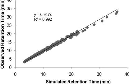
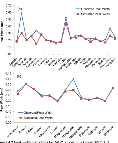
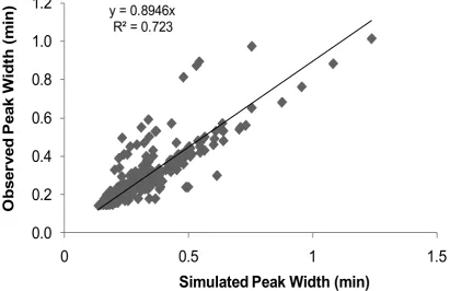
segmented isocratic steps. The three algorithms were found to be highly similar in their predictive errors, which were all 4% on average. Peak width modelling was much more difficult due to well known peak broadening processes. Two empirical peak width models were found to be viable for peak width simulation of analyte under complex eluent profiles. The first peak width model measured the compression exerted from each individual step using a weighting function with a compression term calculation. The second peak width model simulated the peak width using only the eluting retention factor under isocratic conditions. Both models were found to deliver predictive errors of 17% on average.

In summary, this study indicated that the retention time simulation of analytes using the newly derived models can be predicted with an average error of ≤ 4%, which is very close to the target acceptable average error limit of 2.5% required for reliable prediction. The second aspect of the modelling process investigated the broadening of the chromatographic during a separation. It was found that the width of an analyte peak could be simulated reliably using both of the derived models with an average error of ≤ 17%. This can be compared to the error threshold of up to 35% that was determined to be manageable for reliable peak width simulation. Hence, two peak width models investigated were deemed to achieve this target.

Table of Contents

Declaration i

Acknowledgements ii

Statement of Co-Authorship iii

List of Publications Arising from this Research v List of Important Terms, Constants and Abbreviations viii

List of Equations xi

Abstract xvi

Table of Contents xix

Chapter 1 Introduction and Literature Review

1.1 Ion Chromatography 1

1.2 Elution Modes 3

1.2.1 Isocratic Elution 3

1.2.2 Gradient Elution 4

1.3 Retention Time Modelling 10

1.3.1 Soft Retention Time Modelling 11

1.3.2 Hard Retention Time Modelling 13

1.3.2.1 Isocratic Retention Time Models 13

1.3.2.2 Gradient Retention Time Models 15

1.3.2.3 Retention Algorithm for Complex Eluent Profiles 17

1.3.3 Soft Models versus Hard Models 19

1.4 Peak Width Modelling 19

1.4.1 Soft Peak Width Modelling 20

1.4.2 Hard Peak Width Modelling 21

1.5 Optimisation 22

1.6 Simulation and Optimisation Software 28

1.7 Summary 29

Chapter 2 Experimental

2.1 Instrumentation 31

2.2 Reagents 31

2.3 Preparation of Standard Solutions 33

2.4 Properties of IonPac Columns 33

2.5 General Chromatographic Conditions 33

2.6 Random Number Generation for Retention Time

Error Threshold Analysis 35

2.7 Random Number Generation for Peak Width

Error Threshold Analysis 36

Chapter 3 Error Thresholds for Accurate Modelling of the Retention Time and Peak Width

3.1 Introduction 37

3.2 Evaluation of Retention Time Error Threshold 38 3.3 Evaluation of Peak Width Error Threshold 44

3.4 Further Investigation 48

3.5 Chapter Conclusion 52

Chapter 4 Prediction of Analyte Retention for the Elution Profiles Comprising Multiple Isocratic and Gradient Steps

4.1 Introduction 53

4.5.1 Alternative Method for Complex Eluent Profiles

(Method 2) 70

4.6 Prediction of Peak Widths for Complex Eluent

Profiles 76

4.7 Optimisation 78

4.8 Chapter Conclusion 80

Chapter 5 Prediction of Retention Employing the Concept of Analyte Velocity

5.1 Introduction 86

5.2 Retention Time Modelling 86

5.2.1 Isocratic Elution Mode 86

5.2.2 Gradient Elution Mode 89

5.2.2.1 Solution for Retention Simulation of Gradient

Conditions 94

5.2.3 Complex Eluent Profiles (Method 3) 96

5.2.4 Comparison of Predictive Algorithms for Complex

Elution Systems 99

5.3 Peak Width Modelling 102

5.4 Comparison of Simulated and Observed

Chromatograms 105

5.5 Chapter Conclusion 108

Chapter 6 Methodology for porting retention prediction data from conventional-scale to miniaturised ion chromatography systems

6.1 Introduction 109

6.2 Effects of Altering Column Diameters 111

6.4 Recalibration of Retention Database 116 6.5 Prediction of Retention for Different Column

Diameters 120

6.6 Chapter Conclusion 126

Chapter 7 General Conclusions and Future Directions 127

Chapter 1

Introduction and Literature Review

1.1 Ion Chromatography

Ion chromatography (IC) is a powerful analytical technique for the separation and determination of inorganic solutes. IC falls into the general classification of liquid-solid chromatographic methods in which a liquid (called the mobile phase or eluent) is passed over a solid stationary phase and then through a suppression device before entering a flow-through detector (typically a conductivity type). The sample to be separated is introduced into the flowing eluent stream by means of an injection device inserted into the flow-path prior to the column[2].

When a sample is introduced into an IC system, equilibrium is

established for each sample component between the mobile and stationary phases. Thus, for a component, A, this can be written as[2]:

Am⇌ As Equation 1.1

where the subscript m refers to the mobile phase (eluent) and s refers to the stationary phase.

The distribution of component A between the two phases is given by the distribution coefficient, DA, where[2]:

[ ]

[ ]

A A =

D Equation 1.2

The value of DA is dependent on the population of component A in the

stationary and eluent phases[2]. Since the equilibrium shown is dynamic, there is a continual, rapid interchange of component A between the two phases.

Sample components will only progress towards the end of column when they are in the mobile phase. If component A has a large value of DA, it

reach the end of the column. Hence it has a large retention time. Retention can also be expressed in terms of retention factor, k:

Equation 1.3

where Vmis the volume of the mobile phase and w is the weight of the

stationary phase.

The stationary phase for anion analysis usually comprises secondary, tertiary or quaternary ammonium functional groups as anion ion-exchange moieties, whilst sulfonate or carboxylate functional groups are usually employed for cation separations[2].

An anion-exchange material can be expressed as M+E-, where M+ denotes the insoluble matrix material comprising a fixed (positive) charge and E-_{represents the competing ion. When a solution containing an analyte anion,}

A-_{, is injected into the separation column, equilibrium is established between}

the two mobile ions E-_{and A}-_{as follows[2]:}

⇌ Equation 1.4

A single univalent anion A-_{displaces a single univalent counter-ion E}-_.

Thus the equation can be expressed for y moles of Ax-_{exchanging with x}

moles of Ey-_{to give[2]:}

⇌ Equation 1.5

where the subscript m denotes the mobile phase and s denotes the stationary phase.

Therefore, the equilibrium constant of the reaction is given by[2]:

[ ] [ ]

[ ] [ ]

s y -x m

x -y m y -x s E A,

E A

E A =

K Equation 1.6

When a mixture of analytes is injected into an IC system, the analytes will begin interacting with the stationary phase to different degrees depending on their KA,E values, which leads to different rates of progression through the

column. The movement of the analyte relies on the physio-chemical properties, including its size, polarisability, hydrophobicity and charge, the concentration of the mobile phase (MP), the temperature of operating condition, the flow-rate of the system and the morphology of the stationary phase (SP)[2].

The eluent concentration and the stationary phase possess the greatest influence on the retention of a separation. The empirical refinement of chromatographic conditions to accomplish an efficient separation is known as method development and can be very time-consuming.

Method development involves two stages, namely column selection followed by intelligent manipulation of the eluent profile. Column selection is a rapid, but crucial process. Incorrect selection of a column could lead to incorrect selectivity, poor resolution, and unnecessarily long separation times. Eluent profile manipulation is then used to fine-tune the separation of any co-eluting analytes in a separation. Fine-tuning of a separation is a usually iterative process which means that it is often the rate-determining step in method development. This review focuses on manipulation of the elution profile.

1.2 Elution Modes

1.2.1 Isocratic Elution

The first fundamental elution regime is isocratic elution, whereby the eluent composition remains constant throughout the entire separation. The constant eluent strength typically leads to several general elution problems in

separating mixtures containing analytes with widely differing distribution coefficients (DA). On one hand, low eluent concentrations can easily separate

those solutes in the mixture that have smallest DA and they appear as sharp

peaks. Analytes with intermediate DA will be eluted with increased peak width

concentrations result in analytes with high DA emerging in a reasonable time

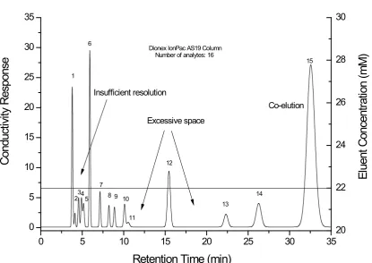
as sharp peaks, however, analytes with small and medium distribution coefficients have insufficient time for separation and thus will be co-eluted with poor resolution[3]. In summary, co-elution, insufficient peak capacity and excessive separation time of the later eluting peaks are the typical problems observed in isocratic separations (Figure 1.1).

1.2.2 Gradient Elution

The second elution mode involves the application of a gradient whereby the mobile phase changes with time either physically or compositionally. Physical gradient elution can be introduced by the altering the temperature, whilst compositional gradient elution is accomplished by varying the concentration of the eluent.

1.2.2.1 Linear Concentration Gradient Elution

Linear concentration gradient elution is performed by varying the eluent concentration linearly over time. This mode is an ideal solution for simple mixtures consisting of a small number of analytes[4].

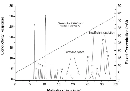
Figure 1.2 shows an illustration of a gradient separation. The

separation commences at low eluent concentration enabling time for the first peaks to separate, while the increasing solvent strength shortens the

separation time and compresses the peak widths of later eluting analytes, which ultimately offers much greater peak capacity[5]. Figure 1.2 shows a more evenly spaced and better-resolved separation compared to the isocratic separation illustrated in Figure 1.1. Early eluters are well resolved and the separation is complete in 33 min compared to 35 min for the isocratic

separation. Notwithstanding these improvements, insufficient resolution and excessive space are still observed.

1.2.2.2 Multi-step Concentration Gradient Elution

Complex eluent profiles generally comprise a number of isocratic and linear gradient steps[5, 6]. Multi-step concentration gradient elution usually

Figure 1.1 Illustration of general problems observed in isocratic separation. The separation consists of 16 analytes eluting in the order of 1-fluoride, 2-propionate, 3-methanesulfonate, 4-chlorite, 5-bromate, 6-chloride, 7-nitrite, 8-chlorate, 9-bromide, 10-nitrate, 11-carbonate, 12-oxalate, 13-iodide, 14-thiosulfate, 15-thiocyanate and phosphate.

0 5 10 15 20 25 30 35

0 5 10 15 20 25 30 35 Conduc tiv ity R es pons e Co-elution Excessive space Insufficient resolution 15 14 13 12 11 10 9 8 7 6 5 4 3 2 1

Dionex IonPac AS19 Column Number of analytes: 16

Retention Time (min)

Figure 1.2 Illustration of general problems observed in gradient separation. The separation consists of 16 analytes eluting in the order of 1-fluoride, 2-propionate, 3-methanesulfonate, 4-chlorite, 5-bromate, 6-chloride, 7-nitrite, 8-chlorate, 9-bromide, 10-nitrate, 11-carbonate, 12-oxalate, 13-iodide, 14-thiosulfate, 15-thiocyanate and 16-phosphate.

0 5 10 15 20 25 30 35

0 5 10 15 20 25 30 35 Conduc tiv ity R es pons e El uent C onc ent rat ion (m M ) 16 Dionex IonPac AS19 Column

Number of analytes: 16

Retention Time (min)

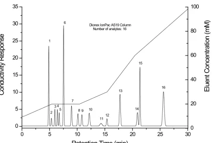
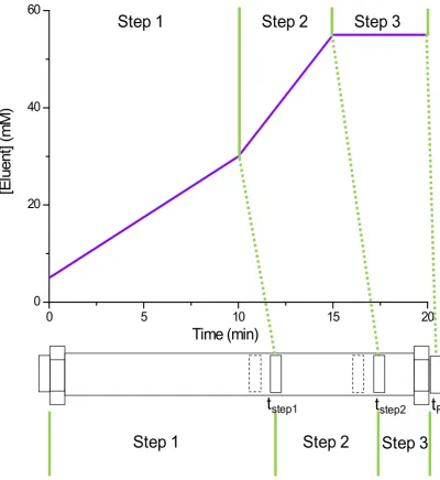
steps. A steep ramp is often introduced at the end to speed up the later eluting peaks and remove the unnecessary space of the separation. An illustration of a separation comprising isocratic and gradient steps is shown in

Figure 1.3. Typical problems of co-elution, insufficient separation and unnecessary space encountered in isocratic (Figure 1.1) and linear gradient (Figure 1.2) separations are better addressed in this elution mode.

One of the major advantages to IC is the routine use of electrolytic eluent generator in which water used as mobile phase feed is converted via an electrolysis step into the desired eluent[7]. An electrolytic eluent generator is typically configured between a pump and separation column. Figure 1.4

shows the configuration of a modern reagent-free ion chromatograph

(RFICTM_{). Eluent generation for isocratic, linear and non-linear gradient, and}

complex elution profiles comprising sequential multiple isocratic and gradient steps is therefore an easy practice. Due to the invention of electrolytic eluent generation module and the applicability of complex eluent profiles on

separating the problematic mixtures, this method has now become the most widely used approach in IC and LC. This is one of the applications where multi-step gradient elution was employed for separation of peptides[4].

1.2.2.3 Non-Linear Concentration Gradient Elution

Non-linear concentration gradient elution utilises a non-linear increase in the eluent concentration, which is a relatively easy exercise to achieve with an electrolytic eluent generator. Non-linear gradients can be defined as either convex or concave[8, 9]. One of the applications employing concave gradient elution is nucleotide analysis[10]. Concave gradient elution is particularly useful in separating a problematic mixture, since it introduces a shallow ramp at the start allowing molecules with low retention to separate with the ramp getting steeper at the end providing strong eluent strength for molecules with large retention.

1.2.2.4 Temperature Gradient Elution

Temperature gradient elution involves varying the temperature of the mobile phase during the elution process. Temperature gradient is an attractive

Figure 1.3 Illustration of a separation consisting of gradient and isocratic steps. The separation consists of 16 analytes eluting in the order of 1-fluoride, 2-propionate, 3-methanesulfonate, 4-chlorite, 5-bromate, 6-chloride, 7-nitrite, 8-chlorate, 9-bromide, 10-nitrate, 11-carbonate, 12-iodide, 13-oxalate, 14-thiosulfate, 15-phosphate and 16-thiocyante.

0 5 10 15 20 25 30

0 5 10 15 20 25 30 35

Dionex IonPac AS19 Column Number of analytes: 16

Retention Time (min)

Figure 1.4 A schematic of a typical reagent-free ion chromatographic system

Column

Detector

Injector

Water

Waste

(water)

Eluent

generator

_Suppressor

H

O → OH

+ H

OH

+ H

H

O

pump and shorter equilibration periods between sequences can be

accommodated. Temperature gradients however have a weaker effect on analyte retention compared to concentration gradients. In addition, a special thermal compartment is required to provide rapid heat transfer to the column and to stabilise the column at elevated temperatures[11]. There are few applications[12-14] employing this technique in either IC or reversed-phase liquid chromatography (LC).

1.2.2.5 Dual-Mode Gradient Elution

Dual-mode gradient elution involves varying the chemical composition and physical characteristics of the eluent simultaneously. Typically, dual-mode gradient elution employs the temperature variations as the physical gradient portion and a concentration multi-step gradient ramp as the chemical

component. This combination offers the best capability in terms of both physical and chemical aspects[15-18]. Dual-mode gradient elution is much more powerful than the application of complex eluent profiles, but its complexity makes optimisation considerably more difficult. This is a new application and only a few research papers[19, 20] have been published in this area.

In summary, a series of elution modes can be used for fine-tuning the separation, however regardless of the type of elution mode, the development of the conditions required must be determined through an optimisation

process. Trial-and-error is the conventional optimisation approach. Typically, a set of designed experiments will be firstly performed, followed by running a further set of experiments to determine the most feasible conditions. More experiments will be carried out as necessary to achieve the desired

separation. This method is an iterative optimisation approach and it requires a large investment of time. Computerised optimisation, (optimisation in-silico) therefore becomes an attractive solution as it is a much more efficient tool for method development.

the resolution in a chromatographic separation need to be modelled mathematically. Resolution is given by[21]:

Equation 1.7

where tR1and tR2are the retention times of the adjacent peaks and w1

and w2are the base widths of both peaks. It is important to note that the peak

widths at half height can also be used to calculate the resolution of a peak pair.

From Equation 1.7, it is obvious that both retention times and peak widths are crucial for optimisation and therefore both need to be modelled accurately. These two parameters can be predicted using both soft and hard models. Soft models are derived independently of any theoretical

explanations. In contrast, hard models are derived from fundamental theory and invariably require knowledge of parameters relating to the characteristics of analytes, stationary phases and eluent profiles for accurate predictions[22].

1.3.1 Soft Retention Time Modelling

Soft models typically aim to fit the best mathematical relationship between the controlled and the measured parameters. Artificial Neural Networks (ANN)[22-30] and genetic algorithms (GA)[31-34] are typically the most popular approaches, and are often referred to as a form of machine learning.

1.3.1.1 Artificial Neural Networks

An ANN is a network consisting of an array of units activated by weighting functions. The basic processing unit in an ANN is a node, which is a

simulated neuron. Multiple nodes can be built into different layers where each node of a present layer is a connection of each node for a previous and future layer. The entire group of nodes constitutes a complete ANN.

nodes and consists of one input layer, one output layer and at least one hidden layer. The complexity of the nodes and layers remains chaotic and fully dependent on the variables and their relationships [22-28]. During the modelling process, the hidden layer nodes and iteration steps of neural network were optimised in order to derive the most accurate retention model. This approach has been applied to limited set of analytes consisting of eight anions and eight cations for predicting the analyte retentions under various isocratic, linear concentration and temperature gradient conditions. The validation was conducted using potassium hydroxide for anion analysis and methanesulfonic acid for cation separations. Bolanca et al.has found that the retention prediction using ANN to be less than ± 2% error on average [22-28].

1.3.1.2 Genetic Algorithm (GA)

Deriving a soft model using a genetic algorithm involves a number of phases. Initially, this approach uses the genetic algorithm selection routine to

determine the subsequent parameters for the training set, followed by

implementing a cross-validated model based on a “leave one out” technique [31-34].

The partial least squares algorithm is an example of a genetic algorithm and it employs the latent variables from a larger set of correlated descriptors in a manner similar to that used in principal component analysis. The algorithm is expressed as follows:

Equation 1.8

where y is the dependent variable (such as retention factor), LViis the

ith_{latent variable and a}

iis the ithregression coefficient corresponding to LVi.

Each latent variable LVican be expressed as a linear combination of

the independent variables xi:

n 3

2 1

i = x + x + x +....+ x

V

L α β δ υ Equation 1.9

where xiis the independent molecular descriptor.

relatively few research works reported in the literature using this approach[31-34].

This approach requires high cost in future maintenance due to lack of theoretical explanations and requirements of large training sets[24, 27]. For instance, an ANN trained for isocratic elution is not compatible for gradient separations. This means that additional data acquisition is required for gradient separations as a new data set must be collected for the training process.

1.3.2 Hard Retention Time Modelling

Hard models are much more informative compared to soft models, but model derivation is a long process. There are a number of mathematical models that have been derived for IC, gas chromatography (GC)[35-39],

reversed-phase liquid chromatography (RPLC)[16-18], and other separation science technologies[40-46].

1.3.2.1 Isocratic Retention Time Models

Retention models for chromatography are derived from factors affecting the elution of analytes, such as their interactions with stationary phase, analyte charge, flow-rate and characteristics of the competing ion.

Madden et al. published two important reviews[47, 48] critically comparing the predictive abilities of a range of isocratic retention models [49-55] suitable for IC. The performance of retention models for isocratic chromatography were comprehensively reviewed over different

suppressed[48] and non-suppressed[47] conditions using single and dual species eluent on different columns. Of the numerous existing models, two approaches, namely the linear solvent strength model, and linear solvent strength model – empirical approach, were found to have the best predictive ability for single (for example, hydroxide) and dual (for example,

The linear solvent strength model (LSSM)[49] is an isocratic retention model capable of predicting the separations consisting of single species eluents and is given by:

Equation 1.10

where k is the retention factor, KA,E is ion-exchange selectivity

coefficient between the analyte and the eluent competing ion, x is the charge of the analyte, y is the charge on the eluent, Q is the effective ion-exchange capacity of the stationary phase, w is the mass of the stationary phase, Vmis

the volume of the eluent species and is the concentration of the eluent.

If this model is employed for isocratic separations consisting of a single competing ion, KA,E, Q, w and Vm can be treated as constants and thus

the model can be simplified to:

Equation 1.11

where a and b are both constants.

A plot of log k versuslog will give rise to a linear relationship with the effective charge of the analyte relative to the competing ion as the slope, b, and the intercept, a, indicating the degree of interaction between analyte and stationary phase. The LSSM has been verified for its high accuracy for isocratic separations employing a single eluent species[49].

The linear solvent strength model – empirical approach (LSSSM – EA) is an extension of the LSSM. It is capable of predicting the separations

consisting of dual species eluent, such as carbonate/bicarbonate. The model is given by following[56]:

Equation 1.12

where f1, f2, f3and f4are isocratic constants and can be determined

charged species. The first portion (f1 + f2 [ET]) of Equation 1.12 accounts for

the solvent strength exerted from singly charged species whilst the second part (f3 + f4 [ET] log [E2-]) integrates the effect from the higher charged

competing ion. Four experimental data points were required to solve for this model. Note that for retention prediction of single species eluent, [E2-_{] is 0}

and Equation 1.12 reverts to Equation 1.11.

These two models (the LSSM and LSSM-EA) and a range of isocratic retention models [49-55] were initially applied to simulate the retention of limited set of anions using Dionex IonPac columns[47, 48] under IC

suppressed and non-suppressed conditions. It was found that the LSSM and LSSM-EA are the best isocratic models for predicting IC separations

consisting of single and dual species eluents respectively. These two models delivered an error of ≤ 5% on average compared to experimental results for retention prediction where only positive errors were observed in the

prediction. It was also found that these two models were more reliable on predicting the IC suppressed separations. The validity of these two models were expanded to extensive sets of analytes, columns and eluents under suppressed conditions in 2002[56] and they are currently employed in the commercial IC optimisation tool, Virtual Column Separation Simulator (Sunnyvale, CA, USA) [56].

1.3.2.2 Gradient Retention Models

Compared to isocratic elution, there are fewer gradient retention models reported in the literature as the gradient elution mode is more complicated than isocratic elution. Existing models have been typically derived from the chemical and physical interactions occurring inside the column, as well as the effect of the change of the eluent strength. All the existing IC models are derivatives of the LSSM.

Equation 1.13 where R is the gradient ramp in mM/min, Cgis a gradient constant and

normally determined from a limited set of experiments, y is the charge of the eluent and x is the charge of the analyte.

This model is valid for single eluent species and a plot of log k versus

log R will give rise to a straight line with a slope of

log R will give rise to a straight line with a slope of [57].

However, the important variables such as flow-rate of the eluent and the initial eluent concentration are not incorporated in this model. As a result, the predictions are limited to gradient separations at fixed flow-rate and starting concentration[57]. This model is currently employed in the commercial IC optimisation tool, Virtual Column Separation Simulator (Sunnyvale, CA, USA)[56].

A highly useful gradient model was proposed in 1974 by Jandera et al.[9, 58] and is expressed as follows:

Equation 1.14 where a is the value of the interaction between stationary phase and the analyte, b is the effective charge of the analyte, B is the gradient ramp in mM/min, tmis the void time, u is the flow-rate, [Ey-]iis the initial concentration,

x is the characteristic shape of the ramp and tRis the retention time. This

model was originally derived for RPLC.

To predict the retention behaviour of analytes, the constants a and b, along with the void time of the column need to be obtained either from isocratic or gradient experimental data.

In 1979, Snyderet al.proposed a gradient model [3, 61] for liquid-solid chromatography and is given by:

Equation 1.15

where kiis the isocratic retention factor observed under isocratic

conditions at gradient initial concentration.

This model has been successfully applied to predict the retention of five benzene derivatives for reversed-phase gradient separations where high correlation was found between the prediction and actual retention data (average error of 0.6%). This gradient model has been incorporated into the commercial optimisation software, DryLab (LC Resources Inc., Walnut Creek, CA, USA)[3, 61]. It is important to note that no research work has been conducted in proving the validity of this model for IC separations.

An important parameter, namely the flow-rate of the system, is not found in the expression. As a result, the validity of this model is limited at a fixed flow-rate.

No critical review is yet to be found in the literature to compare the predictive ability of gradient models for IC separations. Therefore, an evaluation of existing gradient models for IC separations is in the scope of this study.

1.3.2.3 Retention Algorithm for Complex Eluent Profiles

The use of complex eluent profiles provides superior separation ability than using either the isocratic or gradient elution mode. However, the simulation of retention behaviour for a combination of isocratic and gradient steps is

In 2009, Drgan et al.proposed a discontinuous plate model[62]. The underlying concept of this discontinuous plate model remains identical to the LSSM. In this model the separation column was divided into numerous

column segments and the analyte movement is closely monitored in each column segment. This model monitors the analyte movement using the LSSM to understand the distribution of the analyte between the mobile and stationary phases in each column segment and is expressed as follows:

Equation 1.16

where is the function f dependent on the eluent

concentration in the mobile phase of the column segment z after m

movements of the mobile phase, is total amount of eluent in the column segment z after v movement of mobile phase through the column,

denotes the total amount of the analyte in the column segment z after v movement of the mobile phase through the column and is the ratio

between volumes of stationary phase and mobile phase. This algorithm relies on the Newton method to calculate the distribution of the analyte between the mobile and stationary phases in each segment[62]. When the analyte

reaches the end of column after m movement, the segment z can be transposed into retention time.

This highly complex discontinuous plate model delivered an average error of ± 4% for the simulation of retention behaviour of 8 anions on the Dionex AS17 column. However, the time required for predicting a

There are other retention models in the literature, such as those derived for proteins[63-67] and other modes of chromatography [6, 16-18, 68-70] however these models will not be discussed in this present scope.

1.3.3 Soft Models versus Hard Models

There are a number of existing soft and hard models proposed for prediction of retention behaviour in IC separations. Bolanca et al.[24-27] commented that the retention predictions using soft models or ANNs had excellent predictive ability with an average error of 2%. ANNs rely solely on fitting of mathematical expressions empirically with the nodes and hidden layers using large training sets. These models do not provide any theoretical explanations for the separations achieved, and this will be potentially problematic in further maintenance as data re-acquisition and ANN retraining will be required for new systems. In terms of predictive ability, this method is an excellent option for retention time simulation.

As for hard models, these were proposed mainly based on the key factors responsible for manipulating separations. The derivation process for the model can be very time-consuming, while the accuracy is no better than soft models. However, hard models can provide useful chemical relationships and represent elution properties[47, 48, 56]. The main advantages of hard models are that there is no need for a retraining process for new columns as well as they require a minimal set of training sets in comparison to soft models.

In summary, both models offer different strengths and weaknesses for in-silico optimisation. Hard models provide unique fundamental theory for researchers in detailed analysis and justification while soft models can be employed as simulation tools in order to offer a potentially superior predictive ability. Overall, both models should be used to support each other.

1.4 Peak Width Modelling

In isocratic elution mode, peak width is affected by well-known peak broadening processes. These processes cause the band of analyte

an analyte eluted under isocratic conditions can be easily predicted using the rearranged theoretical plate count expression:

Equation 1.17

where N is the theoretical plate number of the analyte.

Peak width in gradient separation is governed by two major factors, namely peak broadening and band-compression. Increasing solvent strength in a gradient elution tends to speed up the trailing edge of the analyte band relative to the leading edge, which results in the compression phenomenon. The broadening of a peak is partially counteracted by this compression effect, which generally results in a narrower peak width across the entire

chromatogram in gradient elution compared to isocratic elution. These two effects have been investigated in order to enable peak width modelling.

1.4.1 Soft Peak Width Modelling

There is only one peak width model reported in the literature for gradient IC separations, which was published by Bolanca et al. in 2009[73]. This

empirical model was derived using an ANN approach. The model measures the peak broadening at three points on the peak; the peak maximum, at half height of the front end of the peak, and at half height of the trailing end of the peak using the following equations:

Equation 1.18

Equation 1.19

Equation 1.20

where aiare regression coefficients with characteristic values for a

1.4.2 Hard Peak Width Modelling

Due to the complex nature of gradient peak width modelling, the predictive ability of existing peak width hard models found in the literature are typically no better than in accuracy compared to the retention models.

In 1974, Jandera et al.[9] proposed a peak width model for predictions in LC and this is based on the column plate number under isocratic

conditions and the instantaneous isocratic retention factor of the solute at the time the peak maximum leaves the column. The model is expressed by:

Equation 1.21

where w is the width of the analyte peak, VRis the retention volume, N

is the isocratic theoretical plate number, is the adjusted retention volume and Vzis the volume of the connecting tubing between the outlet of the

gradient-generating device and the top of the column.

Jandera et al.successfully applied this equation to predict the peak widths of organic analytes in RPLC and the results deviated from

experimental data by ± 25%[9, 58, 74]. This model was further evaluated in a review by Baba et al.[8] for predicting the peak widths of separated

oligonucleotides in IC.

In 1979, Snyder et al.derived a peak width model for liquid-solid chromatography where the relationship is detailed as follows[3].

Equation 1.22

where G is the compression factor which can be calculated from numerical integration.

1.5 Optimisation

Retention time and peak width modelling enables in-silicooptimisation of IC separations to be accomplished. in-silicooptimisation is a two-step procedure. First, a search area (minimum and maximum boundaries) for each parameter (such as initial concentration and gradient slope) that manipulates the

separations needs to be defined. A condition within the defined search area is then systematically/randomly generated, followed by assessing the quality of the potential separation. This process will be repeated until the potential separation meets the defined target. There are a number of strategies that are applicable for optimum searching in the defined area. Each method relies on assigning a numerical quality indicator to predicted chromatograms. The numerical quality indicators are commonly referred to as criterion functions.

A criterion function assigns a numerical rating to each potential

simulated chromatogram. The criterion function typically assesses each peak pair in the chromatogram, or the overall chromatogram. The degree of

separation of two components only is commonly known as elemental criterion. Separation factor, resolution factor, peak-to-valley ratios and area of overlap are all examples of elemental criteria. Elemental criteria for each adjacent peak pair are integrated to give a “composite criterion” that reflects the quality of the entire chromatogram. There are several composite criteria defined in the literature.

A common composite criterion is the sum of resolution criterion function. The equation is given by:

Equation 1.23

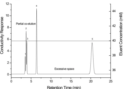
Figure 1.5 Illustration of a 5-component (1-propionate, 2-formate, 3-bromate, 4-bromide and 5-thiocyanate) separation consisting of two general elution problems, namely co-elution and excessive space.

0 5 10 15 20 25

0 2 4 6 8 10 12

Conduc

tiv

ity

R

es

pons

e

Retention Time (min)

Partial co-elution

Excessive space

5 4

3 2

1

36 38 40 42 44

El

uent

C

onc

ent

rat

ion

(m

M

space between peaks 4 and 5 however it does not accurately reflect the partial co-elution between peaks 1, 2 and 3. So this criterion is not useful for the separations consisting of co-elution.

The product of resolution is also a commonly used criterion function. The equation is detailed as[75]:

Equation 1.24

The least resolved peak pair in a chromatogram dominates the

resolution product. The simulated optimum using this criterion function might end up having excessive space between peak pairs while overlooking other conditions where peaks are more evenly spaced[75]. A small resolution product typically corresponds to the co-elution observed in the separation. For example, the resolution product of this separation (Figure 1.5) is 471. A typical resolution product value is considerably large however the resolution product of this separation (Figure 1.5) is relatively small due to the partial co-elution of peaks 1, 2 and 3. Therefore these two peak pairs dominate the resolution product with a small value without indicating the excessive space between peaks 4 and 5.

Normalised resolution product evaluates all peak pairs equally. The equation is expressed as:

Equation 1.25

Minimum resolution is designed to evaluate the least resolved peak pair in the separation. The equation is given by[5]:

Equation 1.26

Baseline resolution of 1.5 is typically employed for an optimum search[5]. It does not measure the excessive space between peak pairs in the separation. For example, the minimum resolution for this separation (Figure 1.5) is 1.2 which corresponds to the least resolved peak pair of peaks 1 and 2. It is less than baseline resolution of 1.5 so this represents more input is required for this mixture. However the minimum resolution does not indicate the excessive space observed in the separation. Therefore this criterion function is not as useful as the normalised resolution product.

Other criteria can also be found in the literature[22, 76, 77] and are useful for other purposes. These criteria are applicable when factors other than resolution need to be evaluated, such as observed number of

components, maximum allowed retention time, retention times of first and final peaks. These factors are implemented to provide more efficient

optimisation for separation. The research interest of this study is to focus on the modelling of retention time and peak width and the criterion functions relying on resolution are found to be providing more information for

optimisation. As a result, other existing criteria will not be discussed further here.

Figure 1.6 A typical example of a 3-level factorial design for two variables

Par

am

et

er

2 (

G

radi

ent

R

am

p)

High

Medium

Low

Medium

_High

Low

Parameter 1 (Initial Concentration)

Hi

gh

M

edi

um

the conditions. The retention time and peak width will then be predicted for all conditions followed by searching for the optimal condition.

It is also possible to employ an iterative tool for the optimum search. Two potential iterative programs, namely Goalseek and Solver, which are both available in Microsoft Excel, can be used for this purpose. Goalseek varies only one parameter sequentially, while Solver can manage multiple parameters simultaneously. After setting the initial conditions and parameters, the retention time and peak width of this input condition will be simulated. If automatically generated and entered into the search system. This process will be repeated until the optimum is found. However, this method has

difficulty managing multiple parameters, especially when there are a number of local minima within the defined region. Therefore, different inputs are highly recommended if numerous variables are involved[5]. Overall, this strategy is much more efficient than full factorial design.

Alternatively, computational algorithms such as the Monte Carlo method, which rely on repeated random sampling to compute the results can be employed for optimisation. The Monte Carlo is the most efficient method in the search for a global optimum for multiple variables using a deterministic algorithm. It is often used for simulating physical and mathematical systems by automated repetition of the mathematical system using pseudo-randomly generated numbers as inputs/conditions. The retention time and peak width will be simulated for all potential conditions and the Monte Carlo algorithm will then identify the global optimum. This method requires no set up time however it is not a commonly used approach in IC method development[78].

The prerequisites of in-silico optimisation are to select appropriate retention time and peak width models, criterion function and strategy for the optimum search. A package consisting of all these tools is an attractive solution. A number of commercial software packages including DryLabTM _[3,

61, 78] and ChromSwordTM _{[78-80] are available for LC optimisation.}

However, they are not the focus of this review and so will not be discussed further. Of relevance is an IC optimisation tool named Virtual Column

1.6 Simulation and Optimisation Software

Virtual Column Separation Simulator is marketed by the Dionex Corporation (Sunnyvale, CA, USA) and it is currently the only commercial simulation and optimisation tool for IC method development. It was originally developed in the Australian Centre of Research on Separation Science (ACROSS) in collaboration with the Dionex Corporation[56].

Virtual Column Separation Simulator provides rapid optimisation as well as a simulation for IC separations on two different column diameters (4 mm and 2 mm) where the prediction on 4 mm separations is available for a variety of columns but the software is not widely available on predicting the 2 mm IC columns. It is capable of predicting separations on single (potassium hydroxide for anion analysis and methanesulfonic acid for cation separations) and dual species (carbonate/bicarbonate) eluents. Retention prediction on dual species eluent is only available for isocratic separations whilst

simulation of retention on single species eluent is available for isocratic and gradient conditions but its predictive ability is limited to a defined range of initial concentration and gradient slope for gradient separations[57]. It employs a total of three existing models for retention time simulation. The linear solvent strength model (LSSM)[49] discussed earlier is employed for predicting an isocratic condition containing single competing ion, while the prediction for an isocratic condition comprising dual eluent species relies on the linear solvent strength model – empirical approach (LSSM – EA)[56], and the model proposed by Rocklin et al.[57] is implemented for predicting

gradient separations. Retention prediction of three models relies heavily on the pre-existing data library embedded in the program and it provides the unique characteristics of each analyte inside the column. The data library which stores all the embedded information is capable to provide rapid and accurate prediction for over 150 ion species and 3 different eluents on 20 different columns at 3 different temperatures[7].

There are several important features not found in this software

such as flow-rate of the system and initial eluent concentration are not found in the model of Rocklin et al. This indicates retention prediction is not feasible for any other flow-rates and starting concentrations. As a result, the Virtual Column Separation Simulator is incapable of simulating any gradient separations outside the defined range (initial concentrations and gradient slopes). In addition, there is no gradient peak width model incorporated in the simulator. All gradient separation is assumed to have the constant theoretical plate count for analyte.

A large range of 4 mm IC column is available for retention prediction in Virtual Column Separation Simulator but the selection of column is very limited for microbore 2 mm IC columns. In addition, there is no prediction available for capillary (0.4 mm) columns which is growing in popularity.

The key limitation of the Virtual Column Separation Simulator is its inability to simulate a complex eluent profile. This method is currently the most widely used approach for separation of problematic samples. This means that the Virtual Column Separation Simulator requires a crucial upgrade.

1.7 Summary

The discussion of all elution modes available in IC suggests that complex elution profiles are currently the most widely employed strategy for trial-and-error optimisation. However, trial-and-error optimisation is losing popularity due largely to time considerations. Computer assisted optimisation is now leading the trend.

Modelling of both retention time and peak width modelling is required for in-silico optimisation.

Scope of the Thesis

The overarching objective of this project was to develop new prediction and optimisation abilities for IC.

the accuracy is important because it permits an informed comparison of the predictive ability of the newly developed models.

The second aim was to devise a real time simulator for complex elution profiles. This simulator was to include both retention time and peak width modelling. This part of the research program involved the incorporation of the existing models as well as formulating new algorithms. The simulators were used to predict the retention times for an extensive set of ions, columns and conditions to validate its applicability.

Chapter 2

Experimental

2.1 Instrumentation

The research detailed herein was performed using three different Dionex ion chromatographs, (Dionex Corporation, Sunnyvale, CA, USA) that were configured according to the specifications listed in Table 2.1. Each IC instrument utilised a configuration established according to the user manual for the instrument. Data acquisition was performed using ChromeleonTM

version 6.80 software.

Table 2.1 Details of three ion chromatograph configurations

Model Number

Gradient Pump

(GP)

Eluent Generation

Module (EGM)

Thermal

Compartment Detector (CD) Conductivity

Auto- sampler

(AS)

DX600 GP50 EG40 AS50 CD25A AS50

ICS3000 ICS3000 _{Dual GP} ICS3000 _EGM detector/chromatography ICS3000

module AS

ICS5000 ICS5000 _{Dual GP} ICS5000 _EGM detector/chromatography ICS5000

module AS

2.2 Reagents

All reagents used in this project are listed in Table 2.2.

Table 2.2 List of Chemicals

Chemical Name Grade Supplier

Sodium Acetate AR May & Baker (Dagenham, England) Sodium Bromide LR BDH (Kilsyth, VIC, Australia) Potassium Chloride AR Ajax (Sydney, Australia)

Sodium Fluoride AR Prolabo (Paris, France) Sodium Formate AR Ajax (Sydney, Australia)

Table 2.2 continues

Chemical Name Grade Supplier

Sodium Oxalate UNK Mallinckrodt (Hazelwood, MO, USA) Sodium Phosphate AR Fluka (Buchs, Switzerland) Potassium Hydrogen

Phthalate AR Ajax (Sydney, Australia)

Sodium Sulfate AR Prolabo (Paris, France)

Sodium Thiocyanate GPR Aldrich (St. Louis, MO, USA) Sodium Thiosulfate AR BDH (Kilsyth, VIC, Australia) Sodium Tungstate AR BDH (Kilsyth, VIC, Australia) Sodium Molybdate AR Ajax (Sydney, Australia) Sodium Perchlorate LR Ajax (Sydney, Australia)

Sodium Pyruvate LR Sigma (St. Louis, MO, USA) Sodium Methacrylate LR Aldrich (St. Louis, MO, USA) Sodium Benzoate AR Aldrich (St. Louis, MO, USA) Sodium Chlorite 80% Aldrich (St. Louis, MO, USA) Sodium Chlorate LR BDH (Kilsyth, VIC, Australia) Potassium Bromate GPR Hopkins & Williams (Essex, England)

Sodium Carbonate AR Ajax (Sydney, Australia) Sodium

Methanesulfonate AR Aldrich (St. Louis, MO, USA) Sodium Chromate AR Aldrich (St. Louis, MO, USA) Sodium Propionate AR Aldrich (St. Louis, MO, USA) Potassium Hydroxide AR Dionex (Sunnyvale, CA, USA) Methanesulfonic Acid AR Dionex (Sunnyvale, CA, USA)

Ammonium Nitrate AR Univar (Sydney, Australia) Barium Chloride LR Ajax (Sydney, Australia) Calcium Chloride LR Ajax (Sydney, Australia)

Cesium Nitrate LR Hopkins & Williams (Essex, England) Lithium Chloride LR Ajax (Sydney, Australia)

Rubidium Chloride LR KOCH (Houston, TX, USA) Methylammonium

Chloride LR Sigma (St. Louis, MO, USA)

2.3 Preparation of Standard Solutions

Standard solutions were prepared by weighing the appropriate amount of the salts listed in Table 2.2 and transferring these to a 200.00 mL volumetric flask and diluting with Milli-Q water (Millipore, MA, USA, 25 o_{C, 18.2 MΩ,).}

Stock solutions were made up to a concentration of 1000 mg/L of the respective ion. Working standard solutions were prepared by diluting the stock solutions with Milli-Q water to concentrations in the range 5 - 30 mg/L. Various mixtures of analytes were prepared based upon their retention times, separation conditions, columns and temperatures chosen.

2.4 Properties of IonPac Columns

There were eight stationary phases (SP) selected for this study, including five anion-exchange SP columns and three cation-exchange SP columns. Full details of the column properties are listed in Table 2.3.

Table 2.3 Properties of IonPac Exchange Columns Used for Suppressed IC

Exchange Column

Column Length

(mm)

Column Diameter

(mm)

Particle Diameter

(μm)

Column Capacity

(μequiv) Hydrophobicity

AS11 HC 250 4 9 290 Medium-Low

AS16 250 4 9 170 Ultra-Low

AS19 250 4 7.5 240 Low

AS19 250 2 7.5 60 Low

AS19 250 0.4 7.5 2.4 Low

CS12A 250 4 8 2800 Medium-Low

CS16 250 5 5.5 8400 Medium

CS16 250 3 5.5 3000 Medium

All columns were equilibrated overnight by flushing with the starting eluent concentration. Detection was achieved using conductivity detection after suppression of the eluent using a self-regenerating micromembrane suppressor (SRS ULTRA-II or SRS300, Dionex Corporation, Sunnyvale, CA, USA).

Analytical Columns: AS11 HC, AS16 and AS19

Guard Columns: AG11HC, AG16 and AG19

Eluent Concentration: will be discussed in subsequent chapters

Eluent Source: Eluent Generator Cartridge (EGC) II Potassium Hydroxide (KOH) with a Continuously

Regenerated Anion Trap Column (CR-ATC)

Temperature: 30 o_C

The general conditions used for cationic analysis in the study were:

Analytical Columns: CS12A and CS16

Guard Columns: CG12A and CG16

Eluent Concentration: will be discussed in corresponding chapters Eluent Source: EGC II Methanesulfonic Acid (MSA) with a

Continuously Regenerated Cation Trap Column (CR-CTC)

Temperature: 40 oC

Flow-rates, injection loop sizes and types of suppression used for all analyses are summarised in Table 2.4.

Table 2.4 List of operating parameters where ASRS: Anion Self-Regenerating Suppressor operated in AutoSuppresion recycle mode, ACES: Anion Capillary Electrolytic Suppressor, CSRS: Cation Self-Regenerating Suppressor operated in AutoSuppresion recycle mode

Column Diameter

(mm) Flow-rate (mL/min) Injection Loop Size (μL) Suppression

4.0 1.00 25.0 ASRS 4mm

2.0 0.25 10.0 ASRS 2mm

0.40 0.01 0.40 ACES

5.0 1.00 25.0 CSRS 4mm