The manifestly gauge invariant Maxwell Dirac equations

(1)

THE MANIFESTLY GAUGE INVARIANT

MAXWELL-DIRAC EQUATIONS

by

Shaun Matthew Inglis, B.Sc. (Hons.)

Supervised by Dr. Peter D. Jarvis and Prof. Lawrence K. Forbes

Submitted in fulfilment of the requirements for the Degree of Doctor of Philosophy

School of Physical Sciences University of Tasmania

(2)

This thesis contains no material which has been accepted for a degree or diploma by the University or any other institution, except by way of background information and duly acknowledged in the thesis, and to the best of my knowledge and belief no material previously published or written by another person except where due acknowledgement is made in the text of the thesis, nor does the thesis contain any material that infringes copyright.

Signed:

(3)

PUBLISHED MATERIAL

The content of chapters 2, 3 and 4 has been published in S. Inglis and P. D. Jarvis Fierz bilinear formulation of the Maxwell-Dirac equations and symmetry reductions, Ann. Phys., 348:176-222, 2014, and the content of chapter 7 was published in S. In-glis and P. D. JarvisAlgebraic inversion of the Dirac equation for the vector potential in the non–Abelian case, J. Phys. A: Math. Theor., 45:465202, 2012. The content of chapter 5 is contained in the article S. Inglis and P. D. JarvisMaxwell-Dirac stress-energy tensor in terms of Fierz bilinear currents currently under consideration by Ann. Phys.

I contributed 80% of the work in these papers and the other 20% was done by Peter Jarvis.

Lawrence Forbes contributed to 20% and I contributed 80% of the numerical work done in sections (6.1) and (6.2), which is intended to be published at a later date.

Signed:

(4)

This thesis may be made available for loan and limited copying in ac-cordance with the Copyright Act 1968

Signed:

(5)

ABSTRACT

We study the Maxwell-Dirac equations, which model the fermionic relativistic elec-trodynamics in the case where the fermion field is itself the source of the electro-magnetic field. This system is formulated by exploiting that fact that the Dirac equation can be algebraically inverted, and the resulting expression for the vector potential in terms of the spinor fields can be directly substituted into Maxwell’s equations.

We work in a formalism where the physical states are described by a set of tensor fields, formed from bilinear combinations of (non-Grassmann) spinor fields and Dirac matrices. This results in a set of manifestly gauge invariant equations that lack such unphysical degrees of freedom. Through the use of Fierz expansions on quadratic spinor combinations, and their associated identities, a large set of interrelationships between bilinear fields can be obtained. This permits the description of the Maxwell-Dirac system in terms of tensor current densities, and their quadratic Fierz identities and continuity constraints.

The resulting set of self-coupled Maxwell-Dirac equations is mathematically in-tractable without further constraint. We show how demanding invariance of the bilinear tensor fields under the action of arbitrary subgroups of the Poincar´e group of rotations, translations and boosts reduces the equations to the point where they are more manageable. In this thesis, we demonstrate in detail how the Maxwell-Dirac equations reduce under several example subgroups.

We also develop the gauge invariant bilinear formalism for the stress-energy tensor, which can be used to calculate physical quantities such as the momentum and mass-energy corresponding to a Maxwell-Dirac solution. The calculation is approached from two independent points of view, namely the Belinfante method and the varia-tional method from general relativity, which we find to be in agreement.

(6)

ACKNOWLEDGEMENTS

I would like to thank Dr. Peter Jarvis for his unrelenting good will and invaluable advice, as well as Prof. Larry Forbes, without whose energy my equations would have remained an unassailable wall of text. My fellow students, Paul Stack and David Horsley deserve to be mentioned also, for listening to my tedious problems and offering insightful ideas, and Graham Legg for his foundational work and guidance. Lastly, my wife Ingrid, whose constant support and companionship made this task far more bearable.

(7)

LIST OF FIGURES

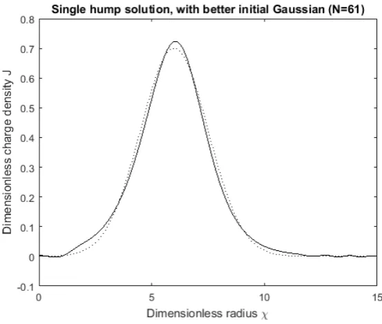
6.1 J(χ) solution, given parameters N = 61, B = 2, µ= 0, σ= 4.1, and R= 25. Default tolerance. Dotted line is the initial Gaussian guess, solid line is the solution function. . . 76 6.2 J(χ) solution, given parameters N = 61, B = 0.7, µ = 6, σ = 1.5,

and R = 25. Function tolerance of 10−12. Dotted line is the initial Gaussian guess, solid line is the solution function. . . 76 6.3 Dimensionless j_a(χ) solutions to the static, spherically symmetric

Maxwell-Dirac equation ODE, where the solid and dotted lines cor-respond to positive and negative signs on the square root term re-spectively. . . 77 6.4 J(χ) solution, given parametersN = 101,B1=B2 = 0.23,µ1= 5.0,

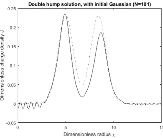
µ2 = 8.4,σ1=σ2 = 0.8 andR= 25. Function and step size tolerance of 10−7. Dotted line is the initialM = 2 double-Gaussian guess, solid line is the solution function for J(χ), and a close approximation of the fullj_a(χ) solution. . . 77 6.5 A comparison ofj_a(χ) obtained from single and double hump

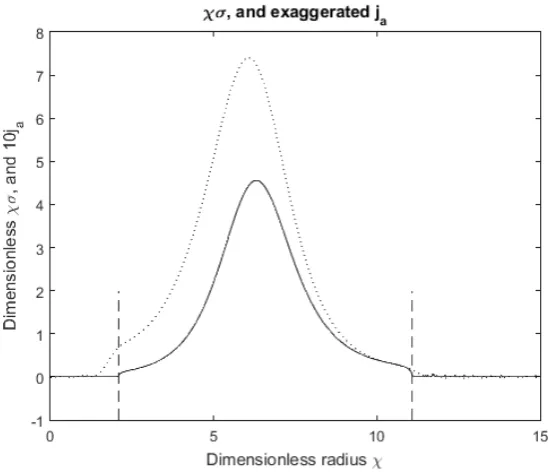
Gaus-sian initial guesses. . . 84 6.6 Comparison of χσ (solid line) with a 10× vertically exaggerated j_a

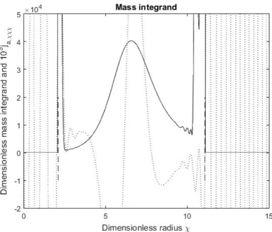
plot (dotted line). The outer boundary of the integration region is indicated by the vertical dashed lines, and is chosen to be where the real part ofχσis non zero. . . 84 6.7 Comparison ofχ2T00 (solid line) with a 105× vertically exaggerated

j_a,χχχ plot (dotted line). The outer boundaries of the integration region, where χσ ≈ 0, are indicated by the vertical dashed lines. Numerical instability ofj_a,χχχnear the edges of the integrated region is apparent. The size of the largest solid spike is∼109. . . 93 6.8 Comparison ofχ2T00 (solid line) with a 105× vertically exaggerated

j_a,χχχ plot (dotted line). The outer boundaries of the integration region, where χσ ≈ 0, are indicated by the vertical dashed lines. Numerical instability ofj_a,χχχnear the edges of the integrated region has been eliminated by setting the derivatives to zero at arbitrary points near the edges. This alteration removes the spikes entirely. . . 94

(12)

LIST OF FIGURES vi

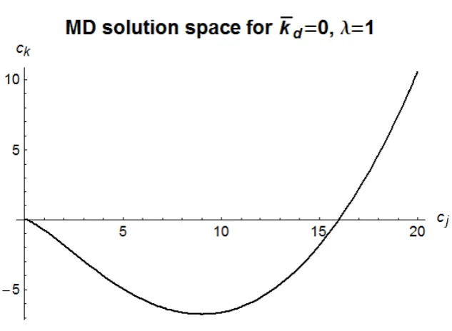
6.9 A plot ofck vs. cj for the case whereλ= 1,kd= 0. . . 94 6.10 A plot of j0 (solid) andj3 (dashed) vs. y for the case where λ= 1,

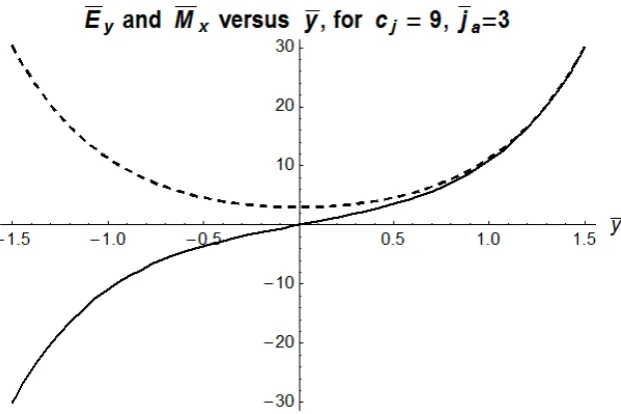
kd= 0, cj = 9 and ja= 3. . . 95 6.11 A plot ofEy (solid) andMx (dashed) vs. yfor the case whereλ= 1,

kd= 0, cj = 9 and ja= 3. . . 95 6.12 A plot of theck= 0 contour when λ= 1, for given cj and kdvalues.

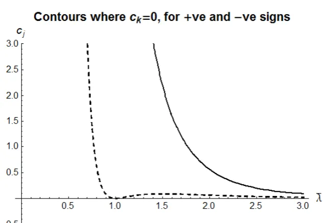
ck < 0 values lie underneath the contour. Note that kd can take negative values, and this graph is symmetric about the horizontal axis. 96 6.13 A plot of the ck = 0 contours as functions of cj and λ for the case

(13)

Chapter 1

Introduction

1.1 The Maxwell-Dirac equations

It is generally understood that the Dirac equation is of central importance in modern physics. The solutions of this equation are four-component objects known as “spinor fields”, usually denoted by ψ, and describe the states of relativistic spin-1/2 parti-cles, such as electrons, positrons and quarks. Following the publication of Dirac’s seminal paper [13], the close correspondence of the Dirac equation with Nature was confirmed dramatically through its predictions of spectroscopic fine structure, and the experimental discovery of the positron. It was, and remains, a triumph of theoretical physics. The Dirac equation for a free particle is

(iγµ∂µ−m)ψ= 0. (1.1) The Dirac equation subsequently went on to play a central role as the exemplar of the matter sector of interacting Abelian and non-Abelian gauge theories in the paradigmatic quantum field theory of particle physics, the Standard Model. The Abelian gauge field here is otherwise known as the electromagnetic vector potential Aµ, and it is introduced by imposing localU(1) gauge covariance on the Dirac equa-tion, whereby the partial derivative term ∂µ is replaced by the covariant derivative term Dµ≡ ∂µ−iqAµ, whereq is the electromagnetic coupling constant. The fact that elements ofU(1) commute is what makes it an Abelian group.

The physical behaviour electromagnetic vector potential itself is described by Maxwell’s equations, which can be solved in the presence (or absence) of electric charges and currents. That is, a given four-current jµ distribution will generate an Aµ field, according to the inhomogeneous Maxwell equations. Similarly, in the U(1) gauge covariant Dirac equation, a given externally applied Aµ field will determine the fermion spinor states ψ. The spinor field is related to the four-current by the defi-nition jµ ≡ψγµψ, to be clarified later. A natural self-coupling between these two sets of equations can be made, by considering the case where the spinor field ψ is itself the source of theAµ field that it interacts with. This is to be contrasted with the “externally applied” Aµ field case, whereby the source of the electromagnetic field lies outside of the distribution in question, and the arbitrarily chosen Aµ configuration determines the form of ψ.

(14)

1.1. THE MAXWELL-DIRAC EQUATIONS 2

One approach to obtaining such a self-coupled system is to formally “invert” the Dirac equation for the gauge field Aµ, such that it is a function of ψ. From this point of view, it is the form of the spinor field which determines the form of the electromagnetic field, thereby acting as the source. When this form of Aµ as a function of ψ is inserted into the inhomogeneous Maxwell equations, we obtain a set of expressions dependent on ψ only: the self-coupled Maxwell-Dirac equations. With regards to the inversion itself, in an early study [16] pointed out that, the Dirac equation can be written in the form

M Aµ=Rµ, (1.2)

where M is a 4×4 complex matrix, containing only Dirac spinor components. Because detM = 0, the four equations are not linearly independent, and so M is not invertible. However, a more recent study by Booth, Legg and Jarvis [7], which included extensions to higher space-time dimensions, demonstrated that the system of linear equations is indeed invertible if strictly real solutions of the vector potential are required.

The success of the algebraic method for inversion for the Abelian gauge field begs the question as to whether such an algebraic inversion is possible for non-Abelian gauge fields. The Dirac equation itself can be extended to include “internal” degrees of freedom, such as isotopic spin, or “isospin”. The simplest example is the Dirac doublet isospinor Ψ, which is composed of two regular four-component Dirac spinors ψi, (i= 1,2). The gauge groupSU(2) acts locally on the doublet degree of freedom, producing a unitary transformation on Ψ by rotating in the doublet space by a phase which varies at each point in spacetime. Such transformations do not commute, so SU(2) is a non-Abelian gauge group. The Dirac equation for Ψ can be made SU(2) gauge covariant in an analogous way to the U(1) gauge group case. That is, we replace partial derivative terms ∂µ with theSU(2) covariant derivativeDµ≡ ∂µ−(ig/2)τ·W, wheregis the coupling constant associated with theSU(2) gauge group. The gauge fields Waµ associated with non-Abelian groups are collectively known as Yang-Mills fields, and are analogous toAµ. The number of internal degrees of freedomaof a Yang-Mills gauge field is determined by theadjoint representation of the gauge group [2].

As we shall demonstrate in chapter 7, the formal inversion can be performed, albeit with some extra non-trivial complications not present in the Abelian case. The interactions in the Standard Model, the electroweakSU(2)×U(1) and strongSU(3) gauge fields are both non-Abelian, so the extra complications associated withSU(2) should also be present when extending the work done here to other gauge fields. Before continuing, it is important to note that here we are working with spinor fields which are non-Grassmann wavefunctions. That is, ψ is to be considered a semi-classical fermion state analogous to the single component wavefunctions of non-relativistic quantum mechanics, and that the components of these spinor fields commute. The necessity for this non-Grassmann treatment of the Maxwell-Dirac equations can be understood by considering the inhomogeneous Maxwell’s equations

∂νFνµ=jµ, (1.3)

(15)

1.2. THE FIERZ BILINEAR FORMALISM 3

consider what happens when we take both sides to the power of five. Since ψα (α= 1,2,3,4) has four components, one for each spinor index α, on the right hand side of the equation each term in a full fifth-order expansion will have at least one repetition of a ψα-component. If these components are Grassmann, then by

{ψα, ψβ}= 0, (1.4)

everything on the right-hand side vanishes, giving

(∂νFνµ)5 = 0, (1.5) implying that the Maxwell field has no source term, and is free. Given this funda-mental contradiction, we must conclude that the correct way to deal with spinor fields in the fully non-linear, non-perturbative Maxwell-Dirac formalism is to treat the spinors as commuting objects.

1.2 The Fierz bilinear formalism

In this thesis, we use a spinor bilinear approach instead of dealing directly with the spinor fields themselves. One example of a spinor bilinear already encountered here is the current density four-vector jµ≡ψγµψ, which is a tensor field composed from a quadratic, or bilinear combination of spinor fields enclosing the 4×4 Dirac matrix γµ_{. Other such bilinears can be produced by replacing the} _γµ _{by other 4}_× basis elements of the Dirac-Clifford algebra, or by further altering the spinor fields by charge conjugating, for example see Appendix A.5.

Due to the unphysical and unobservable phase and gauge ambiguities associated with the spinor field, it is often regarded as a secondary entity. Calculations involv-ing measurable quantities remove such ambiguities through various means, such as gauge fixing, or by forming probability density functions through bilinear spinor combinations. There is a substantial literature on the measurability of spinor wave-functions, with historical origins in the ideas of de Broglie, Bohm, and Pauli. In the case of Dirac theory, we cite Takabayasi [41] as an exponent of the view that indeed the spinor bilinear quantities should be regarded as primary, coordinates of a type of relativistic fluid theory.

(16)

1.3. SYMMETRY REDUCTIONS AND SOLUTIONS 4

a physical state described by the sixteen bilinear tensor fields, the Dirac spinor field is determined up to a phase.

This bilinear reformulation is generalizable to the non-Abelian gauge field case, which we discuss in chapter 7. ForSU(2) doublet isospinors Ψ, matrix combinations such as ΨΨ can be Fierz expanded in the Pauli matrix basis, including the 2×2 identity τ0, for the doublet degree of freedom. Due to the tensor product nature of the expansion, for each Pauli matrix, there is a full Dirac-Clifford expansion as in the ψψ case, such that there aresixty four bilinears altogether. Similarly to the Abelian case, there are Fierz identities relating the isodoublet bilinears, and the Lorentz rank-2 fields Siµν and ∗Siµν can be eliminated. Incidentally, non-Abelian fluid flow was investigated in [5], where an application to a quark-gluon plasma, involving the SU(3) gauge group, was discussed.

There are many other identities involving the sixteen bilinears beyond the funda-mental set [10], which can be derived by using the Fierz expansion along with known identities. The extension of this set of sixteen to other classes of bilinears – such as gauge dependent objects where some of the spinors are charge conjugated (i.e., χ ≡ ψc) or contain derivatives so that the spinor field has a Lorentz index – is a necessary part of the mathematical framework for the description of the Maxwell-Dirac equations in bilinear form, as we discuss in chapter 2. A serious attempt at generalizing the fundamental set of nine Fierz identities to include a larger set of bilinear “currents” was presented by Takahashi [42], although bilinears containing spinor derivatives were discussed only briefly.

In chapter 2, we show how given the inverted form of the Dirac equation, one can derive appropriate Fierz identities to remove the explicit appearance of spinor fields entirely, replacing them with bilinear expressions. In this way, the gauge dependent part of the electromagnetic vector potential Aµ can be isolated to a single term containing the gauge dependent bilinears mµ and nµ, which can then be “picked off”, resulting in a manifestly gauge invariant vector potentialBµ. By introducing a tetrad (or vierbein) of bilinear four-vectors, we show that the electromagnetic field strength tensor Fµν can also be written in manifestly gauge invariant bilinear form, clearing the way for the description of the Maxwell-Dirac system in this formalism.

1.3 Symmetry reductions and solutions

The central aim of this thesis is to provide a solid theoretical basis to aid in the search for solutions to the Maxwell-Dirac equations, and to make substantial progress in obtaining such solutions. Although the Fierz bilinear formulation we develop is valid in the general case, experience with other equations in physics suggests that, almost without exception, interesting solutions are those which possess special symmetry properties. Identifying symmetry constraints is therefore likely to be useful in fil-tering solution types, in addition to aiding in the mathematical tractability of what is an exceptionally difficult problem to solve.

(17)

1.3. SYMMETRY REDUCTIONS AND SOLUTIONS 5

physical observables. Secondly, it allows us to sidestep questions of gauge potentials which are invariant under spacetime symmetry transformations, thus avoiding extra complication. The constraints arising through the imposition of a certain type of symmetry are simply restrictions on the form that four-vectors can take, as well as what independent variables are allowed. To be more precise, we take our symmetry constraints to be those associated with an arbitrary (but fixed) Lie subgroup of the Poincaré group acting on four dimensional Minkowski space-time. All such 158 Poincaré subgroups have been classified up to conjugacy class by Patera, Winter-nitz and Zassenhaus (hereafter, PWZ) [35]. The tabular presentation of Poincaré subgroups and their associated Lorentz and translation generators can be used as a convenient “shopping list” of symmetry constraints which can be applied to our Maxwell-Dirac system.

In chapters 3 and 4, we demonstrate how the Poincaré subgroups given by PWZ can be applied to yield a reduced set of equations. Our work focuses on the Maxwell-Dirac system, but the technique can in principle be extended to other relativistically covariant theoretical models which are written in terms of scalar and four-vector fields. We choose two standard cases, namely spherical and cylindrical symmetry, as well as two non-standard casesP11,2 andPe_13,10from [35], which we call the “screw” and “trans-boost” subgroups respectively. The two non-standard cases each have a free continuous parameter, so they in fact represent infinite families of symmetries. The work done in chapter 3 is somewhat technical, and involves the calculation of the forms of scalar and four-vector fields which are invariant under a given sym-metry transformation. Deriving these forms requires the use of the Lie derivative, which generally describes the change of a tensor field of given rank along a vector field corresponding to the transformation itself. Setting the Lie derivative to zero is akin to imposing that the tensor field be symmetric under the given transformation. Each Poincaré subgroup we work with has a set of generators associated with it, which themselves have an associated transformation vector field and Lie derivative. Restricting ourselves to the cases where the tensor fields are scalar and four-vector fields, for each given subgroup generator we can use the vanishing Lie derivative to obtain a set of linear partial differential equations, which can be solved via the method of characteristics to obtain the invariant forms corresponding to that gen-erator. This process can be applied cumulatively for successive generators, until we eventually obtain forms for scalar and four-vector fields which are invariant under the action of the entire Poincaré subgroup.

(18)

Maxwell-1.3. SYMMETRY REDUCTIONS AND SOLUTIONS 6

Dirac equations when a dominant electrostatic potential A0 was assumed, with no solutions existing for the case where A0 was negligibly small compared with the three-vector potential, Ai. Lisi also numerically obtained an approximate localized solution by neglecting the three-vector potential, arguing that the angular depen-dence of Ai would break the spherical symmetry. After reintroducing magnetic interaction via a perturbation and finding that it had a small effect on angular de-pendence, the full Maxwell-Dirac system was considered, and a normalized localized solution was found. Estaban et al. [17] employed a variational approach to finding localized solutions, and proved that stationary solutions do exist without making any approximations to the electromagnetic vector potential.

With regards to Lisi’s work, our development of the general spherically symmetric case in chapter 4, in particular the reduction of the field strength tensor in subsec-tion 4.1.3, revealed that in general there is no angular dependence for the magnetic field when the vector potential Bµ is spherically symmetric. What was very sur-prising, and is a major outcome of our study, was that a radially dependent form for the magnetic field is implied by the demand of spherical symmetry itself, in the characteristic form of a magnetic monopole with magnetic chargeqm =∓2π/q. De-spite all magnetic terms cancelling from the full self-coupled Maxwell-Dirac system, the presence of the monopole field is a vital component of the spherical symmetry regime, without which it would not exist.

Using the van der Waerden two-spinor formalism, Radford [37] performed a reduc-tion and numerical analysis of the Maxwell-Dirac system under the assumpreduc-tion of a spherically symmetric, static Dirac spinor field, finding that localised compact objects with a shell-like structure exist in this regime. At large distances, a shield-ing effect from the electrostatic charges dominates, and the field from the central charge distribution approaches a Coulombic form. In a follow-up publication [38], Radford proved a theorem stating that stationary spinors (which translate to static bilinears), subject to weak regularity and decay conditions in the asymptotic region, result in strictly localized Maxwell-Dirac solutions which decay exponentially. In section 6.1, we undertake our own investigation of the static, spherically symmet-ric solutions of the Maxwell-Dirac equations, but in the bilinear formalism. We find that the system can be reduced to a single fourth-order, non-linear ODE, for which we show that there is an exact (but unphysical) solution, with a large singularity at the origin. After calculating the equilibrium points of the ODE, we find that the only one of physical interest is j_a,e = 0. Linearizing about the system about this point corresponds to a direct linearization of the system, yielding the weakly non-linear ODE for the function J exactly the same as for j_a, but lacking a square root term of ambiguous sign. Using a set of spectral basis functions, we reformulate the problem to the algebraic one of finding a set of Fourier coefficientsbnthat minimizes a set of Galerkin residualsRn. Using Gaussian-form initial guesses, we obtained the two solutions displayed in Figure 6.5. Similarly to the solution obtained by Rad-ford, we find solutions with a static shell-like structure, but for two “orders” with different numbers of shells. In contrast with Radford [37], our solutions lie out from the origin, and are more densely localized.

(19)

1.4. THE BILINEAR STRESS-ENERGY TENSOR 7

albeit in the more general case where time variation can occur. The requirement of magnetic monopoles is not shared by a subsequent study by Booth and Radford [8] on static cylindrically symmetric solutions. A solution describing a localized Dirac field with a concentric shell structure surrounding a charged axis, as well as finite linear charge density was obtained, and was compared to an equivalent “linearized” system, which lacked the self coupling between the Dirac and Maxwell equations. The relegation of the Maxwell field to an “external” potential resulted in both the localization of the Dirac field and boundedness of the charge density being destroyed. Das and Kay [11] investigated solutions to the Maxwell-Dirac system where the spinor field was assumed to be the form of a plane wave solution to the free Dirac equation. It was found that non-trivial solutions only exist when m = 0, with the additional requirement that associated four vector fields be null. Plane wave solutions were also investigated by Bao and Li [3] as a test case for their broad numerical scheme for the Maxwell-Dirac system, which yielded exact results. On the technical matter of the existence of solutions in general, a very formidable global existence proof to the Cauchy problem for the Maxwell-Dirac equations has been provided by Flato et al. [19], extending upon previous work on the matter by Gross [23].

We should also give an honourable mention to the unpublished work of Legg [31], upon which our current work is inspired, where Poincar´e subgroup invariant solu-tions of the manifestly gauge invariant Maxwell-Dirac equasolu-tions were investigated. Focusing on transitive Poincar´e subgroups that have four-dimensional orbits, Legg found that the only one that resulted in a physically interesting solution wasPe_13,10, what we call the “trans-boost” subgroup, and a reduction of the Maxwell-Dirac system and closed form solution implying hyperbolic distributions as in Figures 6.10 and 6.11 was subsequently presented. Our work in section 6.3 constitutes an independent, alternative confirmation of Legg’s result, with the insight that it cor-responds to a special case in a class of more general solutions, the parametrization of which we discuss in some detail.

1.4 The bilinear stress-energy tensor

When choosing a mathematical construct to model the stress-energy of a given phys-ical system, it appears after investigation that the situation is not entirely straight-forward. Likely, the first model found during any search of the literature is the so-called “canonical form” [22], which is defined as the Noether symmetry current associated with invariance of the Lagrangian density under space-time translations. However, the canonical form has the unfortunate drawback of not being either sym-metric in its two indices, or gauge invariant.

(20)

which are attributed to the spin contribution to the stress-energy.

The variational approach uses the action principle to relate the variation of the Hilbert action of space-time to that of matter, then invoking Einstein’s equations to identify the matter part to the stress-energy tensor. The result is an expression for the stress-energy which is proportional to the functional derivative of the action of matter, with respect to the inverse metric. The presence of the metric ensures that the stress-energy tensor is manifestly symmetric.

Regardless of the independent nature of their derivation, Goedecke pointed out [20] that in the limit of flat space-time, the Belinfante and variational forms of the stress-energy tensor must agree. The equivalence in the integral spin field case was proven by Rosenfeld [40], and Goedecke provided evidence for equivalence in the half-integral spin field case via a series of examples, but was not able to provide a general proof. Such a proof for the half-integral case was published shortly afterwards by Lord [33], using the vierbein formalism.

Much effort has been made to “improve” the stress-energy tensor, either by gen-eralizing it beyond the Belinfante/variational forms, or by altering it so that it is compatible with a given theory. An example of the generalization aspect is the work done by Gotay and Marsden, who model the stress-energy in terms of fluxes of the multimomentum map across space-time hypersurfaces [21]. The Gotay-Marsden stress-energy tensor naturally includes the spin “correction terms” present in the Belinfante formula, but in a more generalized fashion, as well as coinciding with the variational form in the presence of a space-time metric. Work has also been done by Callan, Coleman and Jackiw on making the cut-off dependent symmetric stress-energy tensor compatible with renormalized perturbation theory, by constructing appropriate counter terms in order to make it finite at arbitrarily large cut-off val-ues [9]. The renormalization compatible stress-energy tensor is also compatible with an altered, but phenomenologically consistent, version of general relativity, and sim-plifies the currents associated with scale and conformal transformations in which the stress-energy appears.

The work we present in chapter 5 can be viewed as analogous to one of Goedecke’s examples, namely the coupled Maxwell-Dirac fields, but in an alternate formalism where the spinor fields are mapped bilinearly to a set of tensor fields.

(21)

analogous bilinear form, using a contracted form of the Fierz identity obtained in section 5.1.2. A brief review of how the variational stress-energy is obtained is then given. Then, using the general relativistically covariant form of the bilinear Dirac Lagrangian, the variational stress-energy is obtained, and is found to be in agreement with the Maxwell-Dirac-Belinfante tensor.

(22)

Chapter 2

Maxwell-Dirac Theory and Gauge

Invariant Formulation

We now introduce the theoretical content of this thesis, by showing explicitly how the Maxwell-Dirac equations are formulated in terms of bilinear tensor fields. We begin by demonstrating the inversion of the U(1) gauge covariant Dirac equation for the electromagnetic vector potential. It should be understood that the concerns raised by Eliezer regarding the invertibility of the Dirac equation [16] have been addressed by Booth, Legg and Jarvis [7] by regarding the gauge field as a real ob-ject. There is an alternative inverted form of the gauge field, which follows by an analogous calculation involving dual objects, but we do not present this calculation explicitly here. It is important to note however, that we have found from experi-ence that both dual (containing γ5 terms) and their non-dual counterparts have to be considered during “bilinearization”, whereby spinor-dependent expressions are bilinearly mapped to the analogous representative set of tensor fields.

The Fierz expansion, a concept central to the obtaining of bilinear expressions from quadratic 4×4 spinor objects, such as ψαχβ, is presented. The Dirac spinor in-dices α and β both run from 1 to 4, and denote a degree of freedom distinct from Minkowski spacetime. The process for obtaining the bilinearized form of the Dirac equation is then outlined, which primarily involves the derivation of appropriate Fierz identities to replace the explicitly spinor-dependent objects appearing in Aµ. A major advantage of the bilinear approach then becomes apparent, whereby the gauge-dependence of the gauge field Aµ _{is distilled into a single term, which can be} removed by defining a new gauge-independent field Bµ.

What comes next is the essence of the self-coupled nature of the Maxwell-Dirac system, in that we insert the bilinear expression for Aµ, the inverted Dirac equa-tion, into the electromagnetic field strength tensor Fµν, which itself represents the electromagnetic field in the relativistically covariant form of Maxwell’s equations. It is well known that Fµν, the “four-curl” ofAµis a gauge invariant object, but we can take a step further, and rewrite it as a manifestly gauge invariant object, in which only terms understood to be gauge independent explicitly appear. This can be done by defining the tetrad, or “vierbein”, of four four-vector bilinears, and using a known Fierz identity to eliminate the gauge-dependent terms. We conclude the

(23)

2.1. DIRAC EQUATION INVERSION 11

chapter with a summary of the equations constituting the Maxwell-Dirac system in manifestly gauge invariant bilinear form.

2.1 Dirac equation inversion

The Dirac equation is the relativistic wave equation for spin-1/2 particles, such as electrons. For fermionic particles of charge q interacting with an electromagnetic field, we require solutions to the Dirac equation form-invariant under aU(1) Abelian gauge transformation, given by

(iγν∂ν−qγνAν−m)ψ= 0. (2.1) Conventions for Dirac-Clifford algebra and spinor manipulations are given in ap-pendix A. Our goal is to isolate the vector potential Aµ. Rearranging gives us

γνψAν =q−1(iγν∂ν−m)ψ. (2.2) We can form a bilinear spinor expression by multiplying byψγµfrom the left. Using the Dirac identity (A.10), our expression becomes

ψψAµ−iψσµνψAν =q−1[iψγµγν(∂νψ)−mψγµψ]. (2.3) In order to eliminate the second term on the left-hand side, turn to the charge conjugate Dirac equation, which is similar in form to (2.1), but with the sign of the charge reversed:

(iγν∂ν+qγνAν−m)ψc= 0. (2.4) The charge conjugate spinor is defined in terms of the regular spinor as [26]

ψc=CψT = iγ2γ0ψT. (2.5) Similarly rearranging and left-multiplying by ψcγµ, then applying the appropriate charge conjugation identities in appendix A.4, gives

−ψψAµ−iψσµνψAν =q−1[i(∂νψ)γνγµψ+mψγµψ]. (2.6) Subtracting (2.6) from (2.3) and again using (A.10), gives us the inverted form of the Dirac equation

Aµ= 1 2q

i[ψ(∂µψ)−(∂µψ)ψ] +∂νsµν−2mjµ

σ , (2.7)

where we have used the shorthand notation for Dirac bilinear tensors, listed in appendix A.5. There is an alternative inverted form for the Dirac equation, which involves left-multiplication of (2.1) by ψγ5γµ to form bilinears. Following the same steps as above yields the expression

Aµ= 1 2q

i[ψγ5(∂µψ)−(∂µψ)γ5ψ] +∂ν∗sµν

(24)

2.2. FIERZ IDENTITIES 12

which lacks a mass-dependent term. In addition to these inversions, we can derive other expressions by left-multiplying (2.2) and its charge conjugate analogue by ψΓ andψcΓ respectively, for general elements Γ of the Dirac-Clifford algebra, then adding or subtracting the two equations. Among the resulting expressions are the continuity equation ∂µjµ = 0 and the current-field coupling jνAν. The full list of expressions obtained from “bilinearizing” the Dirac equation is given in appendix B.

2.2 Fierz identities

It is well known that quadratic relationships between Dirac bilinears of the form χΓRψ, where ΓRrepresents the sixteen basis elements of the Dirac-Clifford algebra ΓR={I, γµ, σµν, γ5γµ, γ5}, can be derived via a Fierz expansion of the product of two Dirac spinors in this basis

ψχ= 16 X R=1

aRΓR= (1/4)(χψ)I + (1/4)(χγµψ)γµ+ (1/8)(χσµνψ)σµν

−(1/4)(χγ5γµψ)γ5γµ+ (1/4)(χγ5ψ)γ5. (2.9) Here, aR are the numerical coefficients multiplied by the Dirac bilinears. This expansion is inserted into products such as jµkν ≡ ψγµ(ψψ)γ5γνψ, for example. Experimenting with different combinations of bilinears, and combining the result-ing equations yields many different interrelationships. Many Fierz identities are summarized in [42] and [10], but the most important for our purposes are

jνjν =−kνkν =−mνmν =−nνnν =σ2−ω2, (2.10) jνkν =jνmν =jνnν =kνmν =kνnν =mνnν = 0, (2.11) µνρσjρkσ =mµnν −mνnµ, (2.12) sµν =

(σµνρσ−ωδµνρσ)jρkσ

σ2₋_ω2 , (2.13)

∗_s

µν =

(ωµνρσ−σδµνρσ)jρkσ

σ2₋_ω2 . (2.14)

This method can be extended to the SU(2) spinor doublet case by building into (2.9) an expansion over the Pauli matrices, including the 2 ×2 identity matrix. Analogous non-Abelian expressions to (2.13) and (2.14) are derived in section 7.2 via the use of such expansions.

2.3 Vector potential

(25)

2.3. VECTOR POTENTIAL 13

[ψ(∂µψ)−(∂µψ)ψ] terms. We can then easily pick off the gauge dependent parts (mµ and nµ), to define a gauge-invariant vector potential, which we denoteBµ. A Maxwell-Dirac formalism, completely in terms of manifestly gauge invariant tensors is then derived.

This approach is in the spirit of Takabayasi [41], whose philosophy regarded a rel-ativistic quantum mechanical formalism strictly involving only “observables”, such as tensors, as being preferable to one where somewhat “unphysical” objects such as spinors are explicitly included. A detailed derivation of Bµ is given in appendix C, but we give a brief overview here.

First, take the sum of the two versions of the inverted Dirac equation (2.7), (2.8), and divide by 2

Aµ= 1 4q

i[ψ(∂µψ)−(∂µψ)ψ]ω+ i[ψγ5(∂µψ)−(∂µψ)γ5ψ]σ

σω +

∂νsµν

σ +

∂ν∗sµν ω

−2mjµ

σ

. (2.15)

The appropriate tensor forms needed to replace the spinor terms are jν₍_∂

µkν) and mν(∂µnν). Consider the first tensor:

jν(∂µkν) =ψγνψ·(∂µψ)γ5γνψ+ψγνψ·ψγ5γν(∂µψ). (2.16) Fierz expanding both terms and rearranging gives

jν(∂µkν) = (2/3)[ψ(∂µψ)−(∂µψ)ψ]ω−(2/3)[ψγ5(∂µψ)−(∂µψ)γ5ψ]σ−(1/3)kν(∂µjν). (2.17) We must also consider the Fierz expansion ofkν(∂µjν) in order to eliminate it from the expression, which after rearrangement is given by

kν(∂µjν) = (2/3)[ψγ5(∂µψ)−(∂µψ)γ5ψ]σ−(2/3)[ψ(∂µψ)−(∂µψ)ψ]ω−(1/3)jν(∂µkν). (2.18) Using these two equations yields the new Fierz identity

jν(∂µkν) =−kν(∂µjν) = [ψ(∂µψ)−(∂µψ)ψ]ω−[ψγ5(∂µψ)−(∂µψ)γ5ψ]σ. (2.19) In order to eliminate both of the bracketed spinor terms, we require another inde-pendent expression involving them. Such an expression is provided by mν(∂µnν), which in spinor form is

mν(∂µnν) = (i/4)[ψcγνψ·(∂µψ)γνψc+ψcγνψ·ψγν(∂µψc)−ψcγνψ·(∂µψc)γνψ

−ψcγνψ·ψcγν(∂µψ) +ψγνψc·(∂µψ)γνψc+ψγνψc·ψγν(∂µψc)

−ψγνψc·(∂µψc)γνψ−ψγνψc·ψcγν(∂µψ)]. (2.20) Fierz expanding the individual terms, and applying the appropriate charge conjugate and complex conjugate bilinear identities from appendix A, we obtain

mν(∂µnν) = (i/4){2[ψ(∂µψ)−(∂µψ)ψ]σ−2[ψγ5(∂µψ)−(∂µψ)γ5ψ]ω

(26)

2.3. VECTOR POTENTIAL 14

Performing another round of Fierz expansions on the last two terms eventually provides us with another Fierz identity

[ψγν(∂µψ)−(∂µψ)γνψ]jν =−[ψγ5γν(∂µψ)−(∂µψ)γ5γνψ]kν

= [ψ(∂µψ)−(∂µψ)ψ]σ−[ψγ5(∂µψ)−(∂µψ)γ5ψ]ω, (2.22) which gives us our desired identity

mν(∂µnν) = i[ψ(∂µψ)−(∂µψ)ψ]σ−i[ψγ5(∂µψ)−(∂µψ)γ5ψ]ω. (2.23) It can be shown via a similar process that

mν(∂µnν) =−nν(∂µmν). (2.24) From substitution and rearrangement of (2.19) and (2.23), we get the expressions needed to eliminate spinors from the inverted Dirac equation entirely

[ψ(∂µψ)−(∂µψ)ψ] =−(σ2−ω2)−1[jν(∂µkν)ω+ imν(∂µnν)σ], (2.25) [ψγ5(∂µψ)−(∂µψ)γ5ψ] =−(σ2−ω2)−1[jν(∂µkν)σ+ imν(∂µnν)ω]. (2.26) Combining these two identities in the form they appear in (2.15), we get

{i[ψ(∂µψ)−(∂µψ)ψ]ω+ i[ψγ5(∂µψ)−(∂µψ)γ5ψ]σ}(σω)−1 = 2m

ν₍_∂ µnν) σ2₋_ω2 −

ijν(∂µkν) σ2₋_ω2

σ2+ω2 σω

. (2.27)

Substituting into (2.15), we obtain an expression for Aµ exclusively in tensor form Aµ=

1 4q

2mν(∂µnν) σ2₋_ω2 −ij

ν₍_∂ µkν)

σ2+ω2 σω(σ2₋_ω2₎

+∂νsµ ν

σ +

∂ν∗sµν

ω −

2mjµ σ

.

(2.28) We can improve on this by substituting (2.25) and (2.26) into (2.7) and (2.8) re-spectively, then subtracting and rearranging, obtaining a consistency condition for the Dirac equation in tensor form

ijν(∂µkν) = 2mωjµ+σ∂ν∗sµν−ω∂νsµν. (2.29) Substituting this into (2.28), we obtain after some algebraic manipulation, the final form of the inverted Dirac equation in tensor form

Aµ= 1 2q

mν₍_∂

µnν) +σ∂νsµν−ω∂ν∗sµν−2mσjµ

σ2₋_ω2 . (2.30)

We define the gauge invariant vector potential simply by subtracting the only gauge dependent part from Aµ

Bµ=Aµ− 1 2q

mν(∂µnν) σ2₋_ω2 =

1 2q

σ∂νsµν −ω∂ν∗sµν−2mσjµ

σ2₋_ω2 . (2.31) The Fierz identities (2.13) and (2.14) can be used to eliminate the rank-2 tensors from the Bµexpression entirely. With a small amount of work, we find that

(27)

2.4. THE TETRAD OF BILINEARS 15

+δµνρσ[(∂νσ)ω−σ(∂νω)]jρkσ}(σ2−ω2)−2−(1/q)mσjµ(σ2−ω2)−1. (2.32) It is apparent that Bµ is only finite when σ2 −ω2 6= 0. It is perhaps appropriate to mention here that a common alternative definition of the pseudoscalar bilinear [10], [41] is $=ψiγ5ψ, so performing a change of variables, we would have in the denominatorσ2+$2. Since$is real [10], implying thatωis purely imaginary, the denominator only vanishes for σ and ω vanishing independently. Additionally, we have the condition that σ2₋_ω2 _≥_0.

2.4 The tetrad of bilinears

Here we make the claim based on (2.10) and (2.11) that the four mutually orthogonal four vector fields jµ,mµ,nµ and kµ constitute the columns of a tetrad [31]

tµα= (σ2−ω2)−1/2[jµ, mµ, nµ, kµ]. (2.33) µ = 0,1,2,3 is the spacetime index as usual, and α = 0,1,2,3 labels the columns, withα= 0 denoting the timelike fieldjµandα= 1,2,3 denoting the spacelike fields, mµ,nµ and kµ respectively. Gauge transformations can be thought of as rotations in themµ−nµplane. The coefficient (σ2−ω2)−1/2 behaves as a normalizing factor. Now consider the contraction of two tetrads via the µindex

tαµtµβ = (σ2−ω2)−1    

jµjµ jµmµ jµnµ jµkµ

−mµjµ −mµmµ −mµnµ −mµkµ

−nµjµ −nµmµ −nµnµ −nµkµ

−kµjµ −kµmµ −kµnµ −kµkµ    

=δαβ, (2.34)

which in matrix notation is simply (ηtTη)t =I, implying that (ηtTη) = t−1. Putting the inverse tetrad on the right, and labeling the indices appropriately gives us

tµαtαν = (σ2−ω2)−1(jµjν−mµmν−nµnν −kµkν) =δµν, (2.35) an identity which we will find useful in the next section. Taking the derivative of (2.34) and rearranging gives

tνα(∂µtνβ) =−tνβ(∂µtνα), (2.36) which is antisymmetric in α and β. In fact, this is a generalization of (2.19) and (2.24), which were originally derived via the Fierz expansion method. A result of the antisymmetry is that if α =β, the term vanishes, which tells us that the four vector fields multiplied by the normalizing factor (σ2−ω2)−1are orthogonal to their own partial four derivatives. Substituting the components of the tetrad for α =β into (2.36) gives an identity in terms of the unnormalized vectors

(28)

2.5. FIELD STRENGTH TENSOR 16

2.5 Field strength tensor

The electromagnetic field strength tensor is defined as

Fµν =∂µAν−∂νAµ. (2.38) This is a gauge invariant tensor, but in this form it is notmanifestly gauge invariant because it explicitly contains the gauge dependent term Aµ. The manifestly gauge invariant Fµν was originally obtained by Takabayasi [41], then again by Legg [31], this derivation mirroring that of the latter. ReplaceAµusing (2.31)

Fµν =∂µBν−∂νBµ+ 1 2q

∂µ

mρ(∂νnρ) σ2₋_ω2

−∂ν

mρ(∂µnρ) σ2₋_ω2

. (2.39) Our goal is to eliminate the gauge dependent terms mµ andnµfrom the expression entirely. Expanding the derivatives in the bracketed term gives us

∂µ

−∂ν

= (∂µm ρ₎₍_∂

νnρ)−(∂νmρ)(∂µnρ) σ2₋_ω2

+m ρ₍_∂

µnρ)∂ν(σ2−ω2)−mρ(∂νnρ)∂µ(σ2−ω2)

(σ2₋_ω2₎2 . (2.40)

Focusing on the left-hand term, if we insert the identityδσρbetween each four vector derivative in the numerator, then expand using (2.35), we get

[(∂µmσ)δσρ(∂νnρ)−(∂νmσ)δσρ(∂µnρ)](σ2−ω2)−1

= [(∂µmσ)jσjρ(∂νnρ)−(∂µmσ)kσkρ(∂νnρ)−(∂µmσ)mσmρ(∂νnρ)

−(∂µmσ)nσnρ(∂νnρ)−(∂νmσ)jσjρ(∂µnρ) + (∂νmσ)kσkρ(∂µnρ) + (∂νmσ)mσmρ(∂µnρ) + (∂νmσ)nσnρ(∂µnρ)](σ2−ω2)−2 = (mσnρ−mρnσ)[(∂µjσ)(∂νjρ)−(∂µkσ)(∂νkρ)](σ2−ω2)−2

−[mσ(∂µnσ)∂ν(σ2−ω2)−mσ(∂νnσ)∂µ(σ2−ω2)](σ2−ω2)−2. (2.41) To get to the first term in the last step, we used the tetrad identity (2.36) to switch the partial derivatives onto the gauge independent tensors, then factorized. The second term in the last step follows from using (2.37) to replace terms like mρ(∂µmρ) with−(1/2)∂µ(σ2−ω2), and using and (2.36) to place all the derivatives onto the nσ vectors. Substituting (2.41) into (2.40), the right-hand term in (2.40) cancels out, leaving us with

∂µ

−∂ν

= (m

σ_nρ₋_mρ_nσ_)[(_∂

µjσ)(∂νjρ)−(∂µkσ)(∂νkρ)] (σ2₋_ω2₎2 .

(2.42) Applying the Fierz identity (2.12), we can eliminate the gauge dependent tensors entirely, giving us the desired expression

Fµν =∂µBν −∂νBµ+ 1 2q

σρκτjκkτ[(∂µjσ)(∂νjρ)−(∂µkσ)(∂νkρ)]

(29)

2.6. MAXWELL-DIRAC EQUATIONS 17

2.6 Maxwell-Dirac equations

In summary, our Maxwell-Dirac system consists of the Fierz identities

jµjµ=−kµkµ=σ2−ω2, (2.44)

jµkµ= 0, (2.45)

the gauge invariant form of the inverted Dirac equation

Bµ= (1/2q){µνρσ[(σ2−ω2)∂ν(jρkσ)−(1/2)jρkσ∂ν(σ2−ω2)]

+δµνρσ[(∂νσ)ω−σ(∂νω)]jρkσ}(σ2−ω2)−2−(1/q)mσjµ(σ2−ω2)−1, (2.46) the manifestly gauge invariant field strength tensor

Fµν =∂µBν −∂νBµ+ 1 2q

σρκτjκkτ[(∂µjσ)(∂νjρ)−(∂µkσ)(∂νkρ)]

(σ2₋_ω2₎2 , (2.47) and the inhomogeneous Maxwell equations

∂νFνµ=qjµ. (2.48)

We can also use two of the physical constraints obtained from manipulating the Dirac equation listed in appendix B, the continuity equation and its pseudovector analogue

∂µjµ= 0, (2.49)

∂µkµ=−2imω. (2.50)

(30)

Chapter 3

Poincar´e Subgroups and Invariant

Tensor Forms

Now that we have obtained our Maxwell-Dirac system, we must consider how we are to go about finding symmetry reductions. Observing equations (2.46)-(2.48), we can see that we have a third-order non-linear coupled set of PDEs; a very formidable system indeed. It is fortunate that most physically interesting situations have sym-metry under a certain subgroup of the Poincar´e group, two prime examples being the spherical and cylindrical symmetries. These particular cases were studied by Radford and Booth [37], [8], with the additional constraint of having a static Dirac field, which assumes that there must exist a Lorentz frame in which there is no cur-rent flow,jµ₌_δ

0µj0. Since their work was done in the gauge dependent two-spinor formalism, a specific gauge was chosen to remove gauge ambiguity. In this study, we will apply these same symmetries to the Maxwell-Dirac system, but since we are working with inherently gauge invariant tensor fields only, we have the advantage of not having to choose any specific gauge arbitrarily, which could result in a loss of generality.

The situations of spherical and cylindrical symmetry are but two of many pos-sibilities for analyzing the structure of the reduced Maxwell-Dirac system in the presence of symmetries. Given that we are dealing with relativistic wave equations compatible with the underlying action of the Poincaré group of transformations on Minkowski space, appropriate symmetries are therefore subgroups of the Poincaré group. The comprehensive classification by Patera, Winternitz and Zassenhaus [35] (hereafter PWZ), identifies all 158 continuous subgroups of the Poincaré group up to conjugacy, and the methods we develop are in principle able to give Maxwell-Dirac symmetry reductions forany of these subgroups. At the Lie algebra level, the PWZ scheme uses the known list Fi, i= 1,2, ...,15 of distinct subalgebras of the Lorentz group Lie algebra, to establish a corresponding classification Pi,j of Poincaré subal-gebras, where the Lorentz partFiis extended by an idealNi,j containing translation generators for some j = 1,2, ..., ni. In addition, there exists a further exceptional set denotedPe_i,j, for certaini, j. Whereas theP_i,j =F_i+N_i,j split over the transla-tion generators, the Pe_i,j =Fe_i+N_i,j do not. Although each Fe_i is isomorphic to its counterpart Fi as a Lie algebra, it is non-conjugate to Fi within the Poincaré Lie

(31)

19

algebra, as its generators are irrevocably “tied up” in linear combinations with the translation generators.

In this thesis we work in the context of all admissible symmetry reductions of the Maxwell-Dirac system, but we illustrate the method with a small selection of test cases. The standard limits of spherical and cylindrical symmetry (subgroups P3,4 and P12,8 in the PWZ list) exemplify subgroups arising from three-dimensional ge-ometry, biased towards a particular reference frame. A subgroup not explicitly covered here, but an interesting extension of the spherical case is that of the hy-perbolic symmetry subgroup SO(2,1), represented in the PWZ list by P4,4. This illustrates the case of a simple, but non-compact Lie algebra, and would make an interesting comparison case to more involved analyses of the SO(3) Maxwell-Dirac symmetry reduction, due to its algebraic similarity. Finally, we take up two cases (with solvable Lie algebras) which specify one-parameter families of symmetries. The first,P11,2, features an unusual “screw” generator, which is a parametric com-bination of a translation and a rotation about the corresponding axis. The second,

e

P13,10 is a non-splitting subalgebra, with a parameter fixing the amount of transla-tion generator entrained in the definitransla-tion of a certain Lorentz generator in a minimal presentation.

In this chapter, we will calculate the scalar and vector field forms invariant under each subgroup, covering the actual Maxwell-Dirac reductions in the next chapter. As mentioned, the spherical and cylindrical cases reduce to a complicated system of nonlinear PDEs, there is no solution for P11,2, and for P13,10 the Maxwell-Dirac system reduces to a set of algebraic relations. Initially, we use the method described by Olver [34] to obtain a reduced set of independent variables, “invariants” hence-forth, jointly invariant under the action of all the generators of the subgroup. It follows that arbitrary functions of the invariants will also be invariant under sub-group transformations, that is, they constitute solutions to the PDEs corresponding to a symmetric infinitesimal group action. Components of the invariant four-vector field must also be solutions to the PDEs corresponding to invariance under the group action. Such a set of differential equations is provided by the Lie derivative [44], which defines the directional derivative of a tensor field of rank (k, l) along the infinitesimal transformation vector fieldξ ≡ξσ∂σ:

LξTµ1µ2...µkν1ν2...νl=ξ

σ_∂

σTµ1µ2...µkν1ν2...νl−(∂σξ

µ1₎_Tσµ2...µk

ν1ν2...νl

−(∂σξµ2)Tµ1σ...µkν1ν2...νl− ... + (∂ν1ξ

σ₎_Tµ1µ2...µk

σν2...νl

+ (∂ν2ξ

σ₎_Tµ1µ2...µk

ν1σ...νl+ ..., (3.1)

with invariance underξ imposed by setting

LξTµ1µ2...µkν1ν2...νl = 0. (3.2)

(32)

3.1. THE POINCAR ´E GENERATORS 20

transforming as a tensor with two covariant Lorentz indices. We do not need to consider tensor fields with k+l > 1 however, since we have shown that Fµν can be described in terms of scalar and four-vector fields of rank (0,0) and (0,1) re-spectively. Scalar and vector fields invariant under the transformation vector field

ξ must solve the respective PDEs

Lξφ=ξσ∂σφ= 0 (3.3)

L_ξΦµ=ξσ∂σΦµ−(∂σξµ)Φσ = 0. (3.4) Solutions to (3.3) are calculated by using the method of characteristics to obtain the characteristic trajectories, which are the group invariants. Arbitrary scalar func-tions of these invariants solve (3.3), as can be confirmed via substitution. Solufunc-tions to (3.4) are obtained along the same lines, but the situation is complicated by the second term, which mixes some of the vector components. We can obtain a charac-teristic system of ODEs involving the Φµcomponents, from which we get algebraic expressions that allow us to make an accurate guess as to what forms components should take for invariance. The guessed solutions are confirmed by substituting into the equations generated by (3.4).

3.1 The Poincar´

e generators

One of the most important groups in special relativity is the Poincar´e group P, which consists of the Lorentz group of rotations and boosts, SO(1,3), as well as the Abelian group of translations in four dimensions,T(4). Since P is a Lie group, we can take infinitesimal translations and rotations, building finite transformations from infinitesimal ones through exponentiation. This allows us to work with the mathematically simpler Lie algebra of the Poincar´e group, L(P), which forms a vector space with the generators as the basis. Subalgebras of L(P) are described in terms of their constituent generators, and are by definition closed under a Lie bracket operation. The six infinitesimal generators of the Lorentz group are defined by

(lαβ)µν =δαµηβν−δβµηαν (α, β = 0,1,2,3), (3.5) with lαβ = −lβα, and an arbitrary infinitesimal Lorentz transformation on the co-ordinate frame is

Λµνxν = [I+ (1/2)ωαβlαβ]µνxν, (3.6) whereωαβ =−ωβα are the six infinitesimal parameters associated with each gener-ator. In explicit matrix form, the Lorentz generators are

l01=    

0 −1 0 0

−1 0 0 0 0 0 0 0 0 0 0 0

   

, l02=    

0 0 −1 0

0 0 0 0

−1 0 0 0

0 0 0 0

   

, l03=    

0 0 0 −1 0 0 0 0 0 0 0 0

−1 0 0 0     ,

l12=    

0 0 0 0 0 0 −1 0 0 1 0 0 0 0 0 0

   

, l13=    

0 0 0 0 0 0 0 −1 0 0 0 0 0 1 0 0

   

, l23=    

0 0 0 0 0 0 0 0 0 0 0 −1 0 0 1 0

(33)

3.1. THE POINCAR ´E GENERATORS 21

The first three generators are boosts along the x,y andz-axes respectively and the bottom three generators correspond to rotations in thex−y,x−zandy−zplanes. Is is easy to show using (3.5) that the Lie bracket of the Lorentz algebra is

[lαβ, lγδ] =ηαδlβγ+ηβγlαδ−ηαγlβδ −ηβδlαγ. (3.8) A commonly used representation of these generators is

K1=−l01, K2=−l02, K3=−l03, L1 =l23, L2=−l13, L3 =l12. (3.9) We define the components of the transformation vector field ξ_X corresponding to generator X, to be ξXµ≡Xµνxν. In the K−L representation, these vector fields are

ξK1

µ₌     x t 0 0    

, ξK2

µ₌     y 0 t 0    

, ξK3

µ₌     z 0 0 t     ,

ξL1

µ₌     0 0 −z y    

, ξL2

µ₌     0 z 0 −x    

, ξL3

µ₌     0 −y x 0     (3.10)

The vector fieldsξPν

µ_{corresponding to the infinitesimal translation operators}_P ν are simply four vectors with componentsδµν that act on the coordinate space additively

Pν ·x: xµ→xµ+εξPν

µ₌_xµ₊_εδµ

ν. (3.11)

The generators of all of the Poincar´e subalgebras are listed by PWZ [35] using an alternative representation to that defined above, but which allows convenient extension to larger subgroups of the conformal group of spacetime transformations, such as the similitude (Weyl) group [35], [36]. It is important to note that if any extensions of the Maxwell-Dirac symmetry reduction to the conformal group are undertaken, the physical system must be restricted to massless particles only. The PWZ Lorentz generators are

B1 = 2L3= 2l12, B2=−2K3 = 2l03, B3 =−L2−K1 =l13+l01, B4 =L1−K2 =l23+l02, B5=L2−K1=−l13+l01,

B6 =L1+K2 =l23−l02, (3.12)

with explicit matrix form

B1=    

0 0 0 0 0 0 −2 0 0 2 0 0 0 0 0 0

   

, B2 =    

0 0 0 −2 0 0 0 0 0 0 0 0

−2 0 0 0    

, B3 =    

0 −1 0 0

−1 0 0 −1

0 0 0 0

0 1 0 0

    ,

B4=    

0 0 −1 0

0 0 0 0

−1 0 0 −1

0 0 1 0

   

, B5 =    

0 −1 0 0

−1 0 0 1 0 0 0 0 0 −1 0 0

   

, B6 =    

0 0 1 0 0 0 0 0 1 0 0 −1 0 0 1 0

(34)

3.2. SPHERICAL SYMMETRY (SUBGROUP P3,4) 22

In this representation, it is appropriate to replacetandzwith the light cone coordi-nates l+≡t+z andl−≡t−z. The transformation vector fields for each generator

are

ξB1

µ₌     0

−2y 2x 0    

, ξB2

µ₌    

−l++l−

0 0

−l+−l−

   

, ξB3

µ₌     −x

−l+ 0 x     ,

ξB4

µ₌     −y 0

−l+ y

   

, ξB5

µ₌     −x

−l−

0 −x    

, ξB6

µ₌     y 0 l− y     . (3.14)

The translation generators in the PWZ representation are

X1 = (1/2)(P0−P3), X2 =P2, X3 =−P1, X4 = (1/2)(P0+P3), (3.15) where X1 and X4 correspond to translations along the l− and l+ axes respectively. The corresponding (constant) vector fields are

ξX1

µ₌    

1/2 0 0

−1/2    

, ξX2

µ₌     0 0 1 0    

, ξX3

µ₌     0 −1 0 0    

, ξX4

µ₌    

1/2 0 0 1/2

   

. (3.16)

There is another B-generator, a composite of B1 and B2, which is present in the PWZ F5 and F11 subalgebras of the Lorentz group, as well as the P5,i and P11,i subalgebras of the Poincar´e group

Bϕ = cosϕB1+ sinϕB2, 0< ϕ < π, ϕ6=π/2. (3.17) This generator corresponds to a simultaneous rotation around, and boost along the z-axis, the so-called “screw” group, S(1). The continuous parameter varies the generator from being almost a pure rotation (ϕ ≈ 0), to an almost pure boost (ϕ ≈π/2). The extreme cases when ϕ → 0+ and ϕ→ π/2−, meaning Bϕ → B1 and Bϕ → B2, are actually Lorentz subalgebras in their own right, and are given the PWZ labelsF12and F13 respectively. The explicit matrix form and vector field forBϕ are

Bϕ =    

0 0 0 −2 sinϕ

0 0 −2 cosϕ 0

0 2 cosϕ 0 0

−2 sinϕ 0 0 0

   

, ξBϕ

µ₌    

−2zsinϕ

−2ycosϕ 2xcosϕ

−2tsinϕ    

. (3.18)

3.2 Spherical symmetry (subgroup

P

3,4

)

The condition for scalar and vector fields to be spherically symmetric is that they be invariant under the action of the SO(3) group, which consists of the three rotation generators L1,L2 andL3. The Lie derivative of a scalar field invariant underL1 is

LL1φ=ξL1

σ_∂

(35)

3.2. SPHERICAL SYMMETRY (SUBGROUP P3,4) 23

which yields the characteristic system dy

−z = dz

y , (3.20)

giving us the L1 invariant ρ= p

y2₊_z2_{. The requirement for invariance under} _L 2 is

L_L₂φ=ξL2

σ_∂

σφ=z∂xφ−x∂zφ= 0. (3.21) To impose that φ to be jointly invariant under L1 and L2, we require that the solution to (3.21) be a function oft,xand ρ. Using the chain rule, we find that the PDE becomes independent from z explicitly

ρ∂xφ−x∂ρφ= 0. (3.22) The characteristic equation is

dx ρ =

dρ

−x, (3.23)

from which we obtain the joint invariantr =px2₊_y2₊_z2_{. Lastly, we require that}

L_L₃φ=ξL3

σ_∂

σφ=−y∂xφ+x∂yφ= 0, (3.24) which is automatically satisfied by φ(t, r). Now consider the four vector field Φµ invariant underL1. From (3.4) forµ= 0−3, we obtain the following PDEs

LL1Φ

0₌₋_z∂

yΦ0+y∂zΦ0 = 0, (3.25a)

L_L₁Φ1=−z∂yΦ1+y∂zΦ1 = 0, (3.25b)

LL1Φ

2₌₋_z∂

yΦ2+y∂zΦ2+ Φ3= 0, (3.25c)

LL1Φ

3₌₋_z∂

yΦ3+y∂zΦ3−Φ2= 0. (3.25d) Likewise, for L2 we obtain

L_L₂Φ0 =z∂xΦ0−x∂zΦ0 = 0, (3.26a)

L_L₂Φ1 =z∂xΦ1−x∂zΦ1−Φ3 = 0, (3.26b)

LL2Φ

2 ₌_z∂

xΦ2−x∂zΦ2 = 0, (3.26c)

L_L₂Φ3 =z∂xΦ3−x∂zΦ3+ Φ1 = 0, (3.26d) and for L3 we get

L_L₃Φ0=−y∂xΦ0+x∂yΦ0= 0, (3.27a)

LL3Φ

1₌₋_y∂

xΦ1+x∂yΦ1+ Φ2= 0, (3.27b)

L_L₃Φ2=−y∂xΦ2+x∂yΦ2−Φ1= 0, (3.27c)

LL3Φ

3₌₋_y∂_xΦ3₊_x∂

yΦ3= 0. (3.27d)

Noticing that Φ0obeys the same set of PDEs asφ, we can immediately conclude that Φ0 =a(t, r). By taking the combination xL_L₁Φi+yL_L₂Φi+zL_L₃Φi fori= 1,2,3, we simplify the other PDEs to the algebraic set

(36)

3.3. CYLINDRICAL SYMMETRY (SUBGROUPP12,8) 24

xΦ3−zΦ1 = 0, (3.28b) yΦ1−xΦ2= 0, (3.28c) giving us the solution Φi=xib(t, r). SoSO(3) invariant four vector fields must have the general form

Φµ=    

a(t, r) xb(t, r) yb(t, r) zb(t, r)

   

. (3.29)

3.3 Cylindrical symmetry (subgroup

P

12,8

)

For tensor fields to be cylindrically symmetric, they must be invariant under rotation around, and translation along, a single axis. Choosing the rotation plane to bex−y, the axis must be z, so the infinitesimal invariance generators are L3 and P3. The scalar field must satisfy the relatively trivial PDEs

L_P₃φ=ξP3

σ_∂

σφ=∂zφ= 0, (3.30)

L_L₃φ=ξL3

σ_∂

σφ=−y∂xφ+x∂yφ= 0. (3.31) The first equation tells us thatφis independent ofz, and from the second we obtain the invariant ρ = px2₊_y2_{. Cylindrical symmetry requires that scalar fields be} functions of tand ρ only. The vector fields must satisfy

LP3Φ

µ₌_ξ P3

σ_∂

σΦµ= 0, (3.32)

as well as equations (3.27a) to (3.27d). We can immediately conclude that Φ0 = a(t, ρ) and Φ3 = d(t, ρ), since they solve the same equations as φ. We can also say that Φ1 and Φ2 are independent ofz, but due to components mixing, they are not pure functions of t and ρ. From (3.27b) and (3.27c), we obtain the respective characteristic systems

dx

−y = dy

x = dΦ1

−Φ2, (3.33a)

dx

−y = dy

x = dΦ2

Φ1 , (3.33b)

obviously implying that

dΦ1

−Φ2 = dΦ2

Φ1 . (3.34)

Integrating and taking into account the fact that arbitrary functions of tand ρ are constant along characteristic curves, we obtain the algebraic constraint

(Φ1)2+ (Φ2)2=f(t, ρ), (3.35) which accepts solutions of the form Φ1 = xb(t, ρ)−yc(t, ρ) and Φ2 = yb(t, ρ) + xc(t, ρ). This gives us the form of the cylindrically symmetric four vector field

Φµ=    

a(t, ρ) xb(t, ρ)−yc(t, ρ) yb(t, ρ) +xc(t, ρ)

d(t, ρ)

   

The manifestly gauge invariant Maxwell Dirac equations