School of Natural Sciences
Markov Models for the Evolution of
Duplicate Genes, and Microsatellites
Tristan Lee Stark
B.Sc. (Hons.)Supervisors: Dr. Ma lgorzata O’Reilly & Assoc. Prof. Barbara Holland
February 2018
iii
Declaration
This thesis contains no material which has been accepted for a degree or diploma by the University or any other institution, except by way of background information and duly acknowledged in the thesis, and to the best of my knowledge and belief no material previously published or written by another person except where due acknowledgement is made in the text of the thesis, nor does the thesis contain any material that infringes copyright.
This thesis may be made available for loan and limited copying and communication in accordance with the Copyright Act 1968.
Signed:
v
Acknowledgements
I can’t overstate my gratitude to my two supervisors Dr. Ma lgorzata O’Reilly and Assoc. Prof. Barbara Holland for their extensive support throughout not only my Ph.D. but my honours before that. You both have been exceedingly generous to me. You have always made time when I have dropped by your offices looking to discuss this or that mathematical or scientific problem, the meticulous edits to drafts you have provided, or matters of bureaucracy. Without both of your consistent input and guidance, this thesis would never have been possible, and I would not have half of the aptitude or enthusiasm for mathematics or science that I have today. Thank you to you both for your care and diligence in all aspects of this mentoring role.
I’d also like to thank everyone from the UTAS theoretical phylogenetics group, all of whom have been engaging colleagues to work with. The group’s regular informal meetings, conference organisation and participation, and generally engaging attitude has made my time in the UTAS mathematics department all the more enjoyable. I’d particularly like to thank Dr. Jeremy Sumner for his useful comments on group theory, and the orbit stabiliser theorem.
Thank you also to my wife Catherine, who, particularly in these last few weeks, has taken great care for me personally. Not only have you born the majority of the burden of my survival, and the running of our household, you’ve also shamed me with your superior LATEX-skills and helped me to fix my most pernicious typographical errors.
You have served as a great mathematical foil over the years, despite your unfortunate lack of interest in the theory of probability. I hope that I serve this function for you as well as you do for me.
vi
Abstract
Duplicate genes and microsatellites are two key sequences in the study of evolutionary genomics. Gene duplication has been identified as a central process driving functional change in genomes, since it creates functional redundancy in the genome and allows for subsequent mutation to occur in the absence of selective pressure. Microsatellites are rapidly evolving sequences which can be studied over much smaller timescales than most other sequences, and are thus key to the study of population demographics and forensic science.
In this thesis we construct mathematical models for the evolution of duplicate genes, and microsatellites, respectively. We analyse the models in order to make scientific predictions, and derive the following novel results.
We introduce and analyse a modified hazard function, which we use to investigate the preservation of gene duplicates. Further, we construct individual-level models, and present a framework for the extension to population-level models. Also, we construct mappings from mechanistically-motivated intuitive models for gene duplicate evolu-tion, to less intuitive models, which have smaller state spaces and hence are more computationally tractable.
Throughout this analysis, we make scientific predictions based on the properties of the models. We find that the pattern of gene duplicate preservation is more consistent with subfunctionalization than with neofunctionalization. This result is of particu-lar scientific interest, since it is the opposite conclusion of earlier work in the gene duplication literature.
Duplicate genes
Several biological models exist for the evolution of a pair of duplicate genes after a duplication event, and it is believed that gene duplicates can evolve in different ways, according to one process, or a mix of processes. Subfunctionalization is a process under which the two duplicates can be preserved by dividing up the functions of the original gene between them. Here, we find that subfunctionalization is highly consistent with the pattern of gene duplicate preservation, in contrast to previous analysis in the literature.
vii
is not a significant contributor to the preservation of duplicates over the timescales during which regulatory subfunctionalization is resolved. Instead, it is likely that neofunctionalization occurs subsequent to previous subfunctionalization, which acts to preserve copies over the longer time frames required for rare beneficial mutations to have any significant probability of occurring.
Analysis of genomic data using sub- and neofunctionalization models has thus far been relatively coarse-grained, with mathematical treatments usually focusing on the phenomenological features of gene duplicate evolution. In contrast, we develop mech-anistically motivated Markov models, and fit directly to duplicate preservation data. We introduce a modified-cause-specific hazard function to analyse the preservation of gene duplicates. In the context of gene duplication, we refer to this as the pseudo-genization rate, owing to the biological interpretation. We analyse the properties of the modified-cause-specific hazard rate in detail, including limit analysis of the general case, and discuss the shape properties of the specific case of the pseudogenization rate. Further, we extend our model for the evolution of a pair of gene duplicates to model a population of duplicate pairs, by modelling the birth of such pairs as a homogeneous Poisson process. We show that the age distribution of preserved duplicates follows an inhomogenous Poisson distribution, with its rate function depending on the individual-level model. We then fit this distribution to count-data of surviving duplicates in the genomes of four animal species.
Additionally, we extend the individual-level model to a model that includes the process of neofunctionalization, and next, to a model of subfunctionalization for families of gene duplicates. Finally, we map these intuitive models, to less intuitive but more computationally tractable models, and discuss a number of related computational considerations.
Microsatellites
viii
(which are level-dependent quasi-birth-and-death processes) that track the length of the sequence as the level variable, and the number of interruptions (purity) as the phase variable. Our models account for the biological process of point mutation, and its observed effect on the rate of slipped-strand mispairing.
We find that modelling microsatellite purity leads to some complications due to the nature of available data. In terms of the initial model, we discover what constitutes a state-dependent bias in the reporting of repeat sequences by Tandem Repeats Finder (or any similar software used to search whole-genomes for microsatellite sequences). Consequently, we construct a modified model such that all states fall into one of two categories — ‘observable states’, against which the reporting algorithm is unbiased, and ‘unobservable states’, which are never reported. We consider two approaches for treating the unobservable states, first to condition on the process being in the observable states, second to treat unobservable states as absorbing. Our initial analysis and underlying biological intuition suggest that transitions from the unobservable to observable states are very rare, and thus we ultimately treat the unobservable states as absorbing.
Additionally, we extend the individual-level model to a population-level model by modelling the birth of microsatellites as a homogeneous Poisson process. We then derive the transient distribution of such model in terms of the individual-level process. This distribution has appropriate relative clock via the inclusion of point mutation. We fit this transient distribution to whole-genome derived sequence data, however we encounter some difficulties in the optimisation owing to the presence of many local optima.
Table of Contents
Table of Contents 1
List of Figures 4
List of Tables 6
1 Introduction 7
1.1 Markov models in evolutionary biology . . . 7
1.2 Gene duplication . . . 8
1.3 Microsatellites . . . 10
1.3.1 Time evolution of microsatellites . . . 12
1.4 Thesis overview . . . 16
2 Mathematical Prerequisites 19 2.1 Markov processes . . . 20
2.1.1 Discrete-time Markov chains . . . 20
2.1.2 Continuous-time Markov chains . . . 24
2.1.3 Absorbing CTMCs . . . 29
2.2 Likelihood and model selection . . . 37
3 Duplicate Pairs Evolving Under Subfunctionalization 43 3.1 A model for the evolution of a pair of gene duplicates . . . 46
2 TABLE OF CONTENTS
3.3 Hazard function and related measures . . . 52
3.3.1 Hazard function . . . 52
3.3.2 Cause-specific hazard rates . . . 52
3.3.3 Pseudogenization rate and survival function . . . 55
3.3.4 Expected rates . . . 58
3.4 Hughes and Liberles approximation to the hazard rate . . . 59
3.5 Shape properties of the pseudogenization rate function . . . 62
3.6 Comparison of pseudogenization rate to existing phenomenological ap-proximations . . . 73
3.6.1 Approximation in Konrad et al. [66] . . . 74
3.6.2 Approximation in Tuefel et al. [117] . . . 78
3.7 Extending the model to a population of duplicate pairs via a Poisson birth process . . . 91
3.8 Fitting the model to genome data . . . 93
3.9 Discussion . . . 98
4 Further Analysis of Duplicate Genes 103 4.1 Sub- and neofunctionalization for a pair of gene duplicates . . . 104
4.1.1 Model when neofunctionalization replaces functionality . . . . 105
4.1.2 Model when neofunctionalization adds functionality . . . 108
4.1.3 Results . . . 115
4.2 Preliminary work modeling the evolution of gene families . . . 121
4.2.1 Model for gene families of fixed sizen . . . 123
4.2.2 Efficiently computing the state space and generator matrix . . 129
4.2.3 An alternative procedure for computing the state space . . . . 132
4.2.4 Model for gene families of dynamic size . . . 135
TABLE OF CONTENTS 3
5 Microsatellites 139
5.1 Initial model . . . 141
5.2 Microsatellite data . . . 143
5.3 An intermediate model . . . 149
5.4 Final model . . . 154
5.4.1 Specifying the model . . . 155
5.4.2 Limiting conditional distribution . . . 157
5.4.3 Extending the model to a population of microsatellites . . . 166
5.5 Fitting the model to genome data . . . 173
5.5.1 Model identifiability, and likelihood optimisation . . . 176
5.6 Discussion . . . 177
6 Conclusions 183
A Tables of Microsatellite Fitting Results 189
List of Figures
1.1 Slipped-strand mispairing in the template strand. . . 11
1.2 Slipped-strand mispairing in the new strand. . . 11
1.3 Slipped-strand mispairing removing an impure repeat. . . 14
3.1 Subfunctionalization (biological) transition diagram. . . 45
3.2 Approximation to the mean rate of pseudogenization. . . 61
3.3 Pseudogenization ratehptq for Example 3.5.1. . . 68
3.4 Pseudogenization ratehptq for Example 3.5.2. . . 70
3.5 Pseudogenization ratehptq for Examples 3.5.3–3.5.5. . . 73
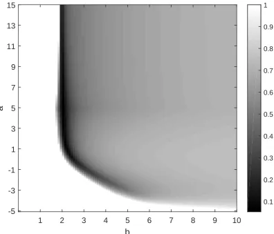
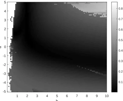
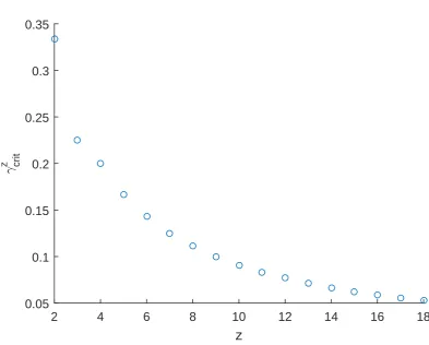
3.6 Critical values γzcrit for various values ofz. . . 74
3.7 Approximation in Konrad et al. [66] with shape parameter c“1. . . . 76
3.8 Approximation in Konrad et al. [66] with shape parameter cą1. . . . 77
3.9 Approximation in Konrad et al. [66] with shape parameter că1. . . . 78
3.10 Average relative difference betweenhTptqand hptq. . . 87
3.11 An example of good performance fittinghptq tohTptq. . . 88
3.12 Numerically minimized average relative difference between hTptq and hptq. . . 89
3.13 An example of poor performance fittinghptq tohTptq. . . 90
3.14 An example of moderate performance fittinghptqtohTptq. . . 91
3.15 Maximum likelihood estimates for γ“ur{uc. . . 94
LIST OF FIGURES 5
4.1 Pseudogenization rate with various rates of neofunctionalization. . . . 118 4.2 Total probability of neofunctionalization. . . 119 4.3 Conditional probability of sub- before neofunctionalization. . . 120
5.1 Repeat number and mismatches for motif-length 3 repeats in lancelet genome. . . 150 5.2 Repeat number and mismatches for motif-length 3 repeats in lizard
genome. . . 151 5.3 Repeat number and mismatches for motif-length 5 repeats in lizard
List of Tables
3.1 Maximum likelihood estimates ande2likelihood intervals for four species. 95
5.1 Genome builds used to generate the TRF datasets for Microsatellite
analysis . . . 144
5.2 Compute-time quartiles to calculate the quasi-stationary distribution. 164 A.1 Results for the full model fitting. . . 189
A.2 Results for the purity-independent model fitting. . . 193
A.3 Results for the constant-bias fitting. . . 196
A.4 Results for the no-bias fitting. . . 199
Chapter 1
Introduction
In this thesis, we construct and analyse several Markov models for processes related to the evolution of duplicate genes, and microsatellites respectively. The evolution of duplicate genes and microsatellites are both areas of significant interest in evolutionary biology, for reasons discussed in Sections 1.2 and 1.3 respectively. We perform both mathematical, and data-driven analysis using whole-genome derived data for both gene duplicates and microsatellites. We focus on the development of mathematical results, which are put into context through discussion of biological interpretations. With this in mind, we start this chapter by putting this work in context with a brief discussion of the importance of Markov models in evolutionary biology as a whole. We then discuss the details of gene duplicate and microsatellite evolution respectively. Finally, we give an overview of the specific contributions presented in this thesis.
1.1
Markov models in evolutionary biology
The theory of evolutionary biology has become increasingly reliant upon the theory of probability, and in particular the theory of Markov processes, since the 1960s. It is easy to see why the theory of probability is so important to evolution — not only are the mutational events underlying practically all evolutionary processes thought to be inherently random, but the complex interactions between different biochemical struc-tures are often not amenable to direct deterministic analysis, and as such statistical models are often required. Pioneering work by Kimura [64], Jukes and Cantor [59], and Felsenstein [39] have enshrined Markov processes at the heart of models for molecular evolution. Since molecular evolution underlies essentially all of evolutionary biology, this has made the theory of Markov processes central to evolutionary analysis. Be-yond just modelling the evolution of proteins or nucleotides, Markov processes have
8 Gene duplication
become a widely used mathematical tool for modelling the evolution of many higher-level genomic processes, including, of particular relevance to this thesis, the evolution of microsatellites.
Despite this, there exists a lot of biological theory which, while amenable, has not been treated with a rigorous Markov-chain based analysis — this is the case for dupli-cate genes. Also, many of the newer or less well-known results from the mathematical theory are rarely applied in evolutionary biology. Non-stationary models are uncom-mon, despite their inherent appeal (with the bigger picture of evolution clearly being a non-stationary process), absorbing processes see little application in the evolutionary biology literature. Likewise, the phase-type and matrix exponential distributions are not often applied.
In this thesis, we discuss our research applying rigorous Markov-chain based analysis to two distinct areas of evolutionary biology. The motivation of this research is two-fold — the primary aim is to analyse the systems and contribute to the understanding of evolutionary biology, and the secondary goal is to introduce some overlooked math-ematical tools to the evolutionary biology literature.
1.2
Gene duplication
Gene duplication has been identified as a key process driving functional change in many genomes. Several biological models exist for the evolution of a pair of duplicates after a duplication event. Gene duplication was first presented as an important process by Ohno [88], who postulated that the emergence of new functions in genomes was enabled by gene duplication. Gene duplication has since been identified as a common occurrence in sequenced genomes [81], and as an important contributor to genome diversification [55; 78].
It is believed that, after duplication, gene duplicates can evolve according to a range of different biological processes. The central process is pseudogenization, where one copy loses its functionality through fixation of deleterious mutations, becoming a so-called pseudogene [56]. In the absence of some pressure to preserve both copies, pseudogenization is thought to be the ultimate fate of any duplicate pair.
Gene duplication 9
ancestral function, and is thus protected from pseudogenization by negative selection. On the other hand, the copy with new functionality could be protected by positive selection, leading to the preservation of both.
Subfunctionalization is a competing hypothesis to explain the preservation of dupli-cates, which was analysed in a series of papers by Force and Lynch [42; 82; 83]. Subfunctionalization is a process of subdividing functions from the ancestral state between the duplicated gene copies, which allows for both copies of the gene to be preserved by selective pressure without the need to invoke positive selection.
To model the evolution of gene duplicates, sub- and neofunctionalization are (usually separately) treated as processes competing with pseudogenization. Thus, under sub-or neofunctionalization models, the ultimate fate of all duplicates is sub- (respectively neofunctionalization) or pseudogenization.
Force et al. [42] described a process which they referred to as duplication-degeneration-complementation (DDC), which is the essential mechanism by which subfunctional-ization is thought to occur. Under the process we have, immediately after some du-plication event, two identical genes, each with a fixed number of mutable regulatory regions. Null mutations occurring in the regulatory regions lead to the complementary degeneration of the pair of genes. Functions which are lost in one copy are retained in the other, and vice versa. While either copy on its own would not be sufficient to retain the functionality of the original duplicated gene, together the two copies can do so. As such there is a selective pressure acting to preserve both copies together in the genome. A side-effect of this is that some redundancy will have developed in the regulatory regions which did not undergo null-mutation in either of the copies, and this could lead to further changes by allowing for mutations which in a single copy would be deleterious, but which will not be selected against due to the redundancy created by subfunctionalization. This could allow for other evolutionary processes to search the space of alleles more freely and lead to subsequent neofunctionalization. Duplicate genes are the subject of Chapters 3 and 4. Our goal was to develop and analyze mechanistically motivated models for the evolution of duplicates after an ini-tial duplication event. Chapter 3 focuses on the analysis of the subfunctionalization process for a pair of duplicates. We build on this work in Chapter 4, where we consider the combined processes of sub- and neofunctionalization for a pair of gene duplicates, and, separately, subfunctionalization for gene families.
10 Microsatellites
convex declining pseudogenization hazard rate most often attributed to neofunction-alization.
1.3
Microsatellites
A microsatellite, or simple sequence repeat, is a strand of DNA which repeats a motif of length 1–6 nucleotides [36]. For example, we may have the string of nucleotides ATATATATAT, which is the motif AT repeated 5 times. Microsatellites undergo a mutation process which leads to a change in the number of repeats, at a rate which is orders of magnitude higher than the rate for other forms of mutation, such as point mutation, insertions and deletions [21]. There is some debate as to how many repeats are required for mutations characteristic of microsatellites to occur. Rose and Falush [99] suggest that the threshold is approximately 8 repeats, however more recently Leclercq et al. found that no such threshold exists [73].
Microsatellites are found in vastly greater density than that which would be implied by random allocation of nucleotides [37]. They are found throughout the genome, in coding and non-coding regions and are ubiquitous in prokaryote and eukaryote genomes [118; 133]. Many microsatellites are thought to evolve neutrally, experiencing no selective pressure [37; 124], and polymerase chain reaction techniques lead to a high availability of microsatellite data by allowing for the production of many copies of DNA sequences.
Neutral evolution, together with high levels of polymorphism resulting from frequent mutation, leads to microsatellites being highly favoured as genetic markers (sequences of DNA occurring at a known locus, used to identify an individual or species) [37; 124]. Hence, microsatellites are of interest in a wide array of population genetics and evolutionary inference applications [101].
Microsatellites 11
Levinson and Gutman [77] proposed that the biological process of slipped-strand spairing was the most likely the dominant process underlying the evolution of mi-crosatellites. Slipped-strand mispairing occurs when, during DNA replication, two strands disassociate and a repeat unit in the nth position of the new strand rehy-bridizes with a complementary repeat unit in some othermthposition of the template strand. A loop of unmatched repeats is formed in one strand and the length of the new strand differs from the template by |n´m|repeats. Whether the new strand is longer or shorter than the template, depends on which of the two the loop was formed in. This biological model is widely accepted as the best description of the underlying process (see e.g. [36; 21; 35]).
A T A T A T A
T A T
A
T A T A T
Loop formed in Template Strand
Template Strand
T A T A T A T A T A T A New Strand
Figure 1.1: Representation of slipped-strand mispairing where the loop is formed in the template strand, shortening the new strand relative to the template.
A T A T A T A T A T A T Template Strand
T A T A T A T
A
T A
T
A T A T A New Strand
Loop formed in New Strand
Figure 1.2: Representation of slipped-strand mispairing where the loop is formed in the new strand, increasing its length relative to the template strand.
Two widely used models in the microsatellite literature are the infinite alleles model [64] and the stepwise mutation model [64]. The infinite alleles model assumes that the num-ber of possible alleles is sufficiently large that any mutation necessarily leads to a state not previously existing in the (finite) population, while the stepwise mutation model is a homogeneous birth and death process taking any integer value. Both models are defined in a more general context than that of microsatellite evolution, and are widely used in a range of evolutionary biology contexts.
12 Microsatellites
observations of microsatellite loci [37], but the model as introduced by Kimura and Ohta [64] is still widely used for population studies.
1.3.1 Time evolution of microsatellites
There are many factors affecting the way a given microsatellite evolves in time. Below we discuss these factors, and the attempts to account for them in existing microsatellite models. The model which we define in Chapter 5 is built upon the general model due to Wu and Drummond [130], which includes a majority of earlier models as submodels. We restrict their model slightly in view of the findings of other analysis, and then extend it to account for the possibility of interruptions in the repeat sequence.
Size of mutation events
Empirical studies of slipped-strand mispairing have been carried out on a variety of species (see for example [58; 43; 15; 119; 14]), and show that the most common mutations are slippage events in which a single repeat unit is gained or lost. Less frequently, slippage events leading to the gain/loss of multiple repeat units are ob-served [33]. There is no general agreement on the distribution of mutation sizes, which it is thought to vary between loci [37], but the consensus is that single repeat unit changes are significantly more frequent that changes involving multiple repeat units.
Microsatellites 13
Length dependence of mutation rate
It has been hypothesised that as the length of a microsatellite increases, there is more opportunity for slippage to occur, and hence that the mutation rate increases. This is confirmed experimentally [127; 14; 75; 15], and Ellegren says in his 2004 review [37] “The single most important factor to affect mutation rate that has so far been discov-ered is microsatellite length.”
Kruglyak et al. [68] proposed a model in which a microsatellite of length i goes to lengthi`1 or i´1 at a rate bpi´1q, where b is a constant. This model provided a good fit for the microsatellites in the yeast genome [67]. Calabrese and Durrett [20] similarly proposed a quadratic model, although Sainudiin [101] found no advantage over the linear model in modelling a Human-Chimpanzee data set. With this in mind, we further restrict the model due to Wu and Drummond [130], upon which we base our model, to allow for only a linear (in repeat number) rate of slipped-strand mispairing.
Contraction vs. expansion — mutational bias
A bias in favour of expansion over contraction for slippage mutations is often ob-served [24; 60; 34; 95]. However, [47; 127] found a bias in favour of contraction. Xu et al. [131] found that the rate of contractions increased exponentially with repeat length while the rate of expansion remained the same. Other studies have similarly shown a change in directional bias with increasing length [51; 43; 47; 91].
14 Microsatellites
Point mutations and microsatellite purity
While slipped-strand mispairing accounts for the majority of microsatellite mutations, all DNA is susceptible to point mutation, whereby a single base nucleotide is replaced with another nucleotide. When a point mutation occurs a microsatellite may become interrupted, for example we might have (AT)30become (AT)12(AC)(AT)17[36]. It has
been observed [57; 38; 129] that mutation rate varies between pure and interrupted repeats. It stands to reason that an interrupted microsatellite may mutate into a pure one, either by the removal of an impure repeat via slipped-strand mispairing, or by a point mutation correcting the impure repeat. Harr et al. [47] showed that purifying mutations do occur. Since microsatellite repeat number was traditionally measured without identifying all nucleotides at the locus in question, point mutations would often go undetected [21] and thus purity data was relatively more difficult to obtain than repeat length data.
A T A T A T A
T
A C
A
T A T A T
Loop forming around an impure repeat.
Template Strand
T A T A T A T A T A T A New Strand
Figure 1.3: Representation of how slipped-strand mispairing might remove an impure repeat.
Microsatellites 15
sequences (in the early days, an extremely costly process) is required.
Due to the repetitive nature of microsatellite sequences, if two appropriate regions flanking the sequence can be identified, primers can be annealed at both ends of the sequence, and the length inferred in a similar manner without identifying the specific nucleotides in the sequence. The length of the sequences can be be inferred directly, along with the size of the repeat unit (since the sequence length would be in integer multiples of the size of the repeat unit, itself in integer multiples of the size of an individual nucleotide). This established the convention in the analysis of microsatellite sequences, which are often still measured in a similar manner, but with the advent of modern DNA sequencing techniques, full sequencing is the norm, and plenty of sequence data is now available.
Attempts to reconcile point mutation and slipped-strand mispairing have led to count-ing schemes that eliminate information about the purity of a sequence in order to maintain both a one dimensional state space in the models, and the convention estab-lished by history of DNA sequencing. For example, Calabrese [20] counts only unin-terrupted repeats, Sibly [106] counts only the left half of an inunin-terrupted repeat and Bell and Jurka [9] tracked either side of an interruption as individual, pure microsatel-lites. Given the effect an impurity has on mutation rate, we expect that accounting for varying levels of purity may improve the models. To that end, in Chapter 5, we extend the model due to Wu and Drummond [130] (with the restrictions mentioned above) to explicitly account for the number of interruptions in the repeat sequence. Aside from those mentioned above, a variety of other factors can influence mutation rate, including sex, the particular repeat motif, and the locus at which it occurs [15; 14; 34]. However, aside from sex, these factors are constant over the life-cycle of a microsatellite. As such, their effects can be accounted for in the choice of parameters of the model, rather than needing to be explicitly accounted for. For example, to account for different mutation rates for varying repeat motifs, a model can be fit to data corresponding to the different motifs.
16 Thesis overview
of the data.
1.4
Thesis overview
In Chapter 2 we provide a summary of some important, well-known results from the theory of Markov processes and statistics, together with some intuitions regarding the interpretation of certain statistical measures. The first part of this summary is used to establish notational conventions and nomenclature for the subsequent chapters, while the later parts highlight some points of particular interest.
In Chapters 3 and 4 we examine gene duplication. The evolution of gene duplicates is a part of the biological theory which has seen relatively little application of Markov processes. We define Markov models for the evolution of the descendents of some gene which has been duplicated by some (unspecified) process. After duplication, the evolution of the resulting copies of the gene is eventually resolved according to one of several competing and/or complementary biological models. Central to this evolution is the process of pseudogenization, whereby copies of the gene can be nonfunctional-ized, and essentially lost to the genome (in the sense that it is no longer functional, and subject to potential deletion, or further degradation). Other processes compete with pseudogenization to fix the copies under selective pressure, ensuring their preser-vation in the genome. We model pseudogenization alongside two different biological models for the preservation of gene duplicates.
In Chapter 3 we consider the evolution of a pair of gene duplicates under the biolog-ical process of subfunctionalization. The duplication-degeneration-complementation (DDC) mechanism, which is detailed by Force et al. [42], describes in precise terms how the mechanics of evolution by subfunctionalization occur for genes after a du-plication event. Early work by Force [42], and Force and Lynch [82; 83] considered subfunctionalization in terms of competing Poisson processes. Subsequent mathemat-ical modelling of the process has been relatively ad hoc [54], employing unjustified approximation where an exact Markov-chain based analysis is possible. We have per-formed such an analysis in our recent paper [109], and we discuss this work and some related unpublished results in Chapter 3. As part of this analysis we introduce a modified-cause-specific hazard rate, and we extend our model for a pair of duplicates to a model for a population of such pairs in order to fit to whole-genome derived count-data.
dupli-Thesis overview 17
cate genes undergoing subfunctionalization by combining an absorbing Markov process describing the evolution of a pair of duplicates with a Poisson duplication process. My contribution to this work included the conception of the model (together with Dr. O’Reilly and Assoc. Prof. Holland), the derivation of a majority of results, coding and data analysis, and writing the majority of the drafts and the final manuscript. Dr. O’Reilly derived the results for ‘Probabilities corresponding to i-th mutational events’ (Section A in Additional file 1 of [109]) as well as ‘Other measures of inter-est’ (Section B.4 in Additional file 1 of [109]), and contributed to the derivation of various other results, wrote part of the initial draft and edited subsequent drafts. As-soc. Prof. Holland contributed to the derivation of various results, edited drafts, and provided biological insights. Assoc. Prof. Liberles edited drafts and provided key bio-logical insights and interpretation of results in the context of gene duplication. These contributions are included in Chapter 3 of this thesis.
In Chapter 4, we introduce some further models related to gene duplication. In par-ticular, we extend the model from Chapter 3 to model gene duplicates evolving under the combined processes of sub- and neofunctionalization. We analyse this model, including extension to the population-level, and fitting to the same dataset consid-ered in Chapter 3. Contrary to previous analysis in the literature, we conclude that subfunctionalization is the dominant mode of preservation of gene duplicates, with ne-ofunctionalization only occurring with any significant probability after earlier subfunc-tionalization. Separately, we extend the model from Chapter 3 to model the evolution of a family of gene duplicates evolving under subfunctionalization. Mechanistically modelling gene families is significantly more complex than pairs of duplicates, and we introduce a procedure for model development which avoids the need to individually consider the many possible transitions the process can undergo. We explicitly consider the problem of evaluating the state space corresponding to gene families of fixed or dynamic size, and outline a procedure to efficiently compute the associated generator matrix.
18 Thesis overview
Existing models are designed to have unique stationary distribution, which is fit to empirical data assumed to be at equilibrium [21]. The prevailing biological the-ory suggests a different picture, with microsatellites thought to undergo finite life-cycles [18; 85; 96; 114; 19]. We extend the individual-level model to a population of microsatellites, and derive a transient distribution with appropriate relative clock to fit to empirical data which is not assumed to be at equilibrium.
Chapter 2
Mathematical Prerequisites
In this chapter, we provide some statements of existing results which will be relied upon throughout the following chapters of the thesis. The main purpose of this chapter is to establish the conventions which we will follow in subsequent chapters, and to provide in-text references for important results. Proofs are not provided for the results stated in this chapter (references to proofs are).
In Section 2.1 we state a selection of key results from the theory of Markov processes. Markov processes are central to this thesis, and readers are assumed to be familiar with the theory. Sections 2.1.1 and 2.1.2 serve primarily to establish notational and nomenclatural conventions which will be followed in the subsequent chapters. As such, throughout Sections 2.1.1 and 2.1.2 statements are given with little exposition. We give some more details in Section 2.1.3 where we discuss absorbing continuous-time Markov chains, which are particularly important to this thesis. For an introduction to the theory of Markov processes, we suggest Ross’s ‘Introduction to Probability Models’ [100], Karlin and Taylor’s ‘An Introduction to Stochastic Modeling’ [115], or Karlkarni’s ‘Modeling and Analysis of Stochastic Systems’ [70]. More advanced topics relevant to this thesis are covered by Neuts’s ‘Matrix-Geometric Solutions in Stochastic Models: An Algorithmic Approach’ [87] and Latouche and Ramaswami’s ‘Introduction to Matrix Analytic Methods in Stochastic Models’ [72]. Further, the review of quasi-stationary distributions provided by van Doorn and Pollett [121] is highly expository for that topic.
In Section 2.2 we discuss the statistical notion of likelihood, and some approaches to the statistical problem of model selection. We employ some results from the theory of model selection at various points in the subsequent chapters, but it is not central to the thesis in the same sense as Markov processes. We assume that readers have a
20 Markov processes
basic familiarity with statistical theory, but we provide some exposition in terms of intutions regarding particular results which we rely upon. For a detailed discussion of likelihood we suggest Rohatgi’s ‘An Introduction to Probability and Statistics’ [98], and for model selection we suggest Burnham and Anderson’s ‘Model Selection and Multimodel Inference’ [17].
2.1
Markov processes
The theory of Markov processes provides a set of powerful probabilistic tools with which to model real world systems, and is ubiquitous in the context of evolutionary biology. Throughout this thesis we will be making frequent use of the theory, and what follows is a summary of a selection of important results.
2.1.1 Discrete-time Markov chains
We are principally interested in the application of continuous-time Markov chains in this thesis. However, Discrete- and Continuous-time Markov chains are closely related, and in keeping with Ross [100], we start by introducing the discrete-time analogue.
Definition 1 (Discrete-time stochastic process).
A discrete-time stochastic process is a sequence X “ tXn : n ě 0u, where Xn is a
random variable for each nPN“ t0,1,2, . . .u. If Xn “i we say that X is in state i
at time n.
The set S of values taken by Xn is called the state space. If S is discrete we say that X is discrete valued.
All of the Markov chains discussed throughout this thesis will be discrete valued.
Definition 2 (Discrete-time Markov chain).
Let tXn : n P Nu be a discrete valued stochastic process in discrete time, with state space S. We say that such a process is a discrete-time Markov chain (DTMC) if it has the property that for any statesi1, ..., in´1, i, jPS and any nPN, we have
PpXn`1 “j |Xn“i, Xn´1 “in´1, . . . , X1 “i1q “PpXn`1 “j |Xn“iq. (2.1)
Markov processes 21
Definition 3 (Time homogeneity).
A time-homogeneous Markov chain is a DTMC for which transition probabilities do not depend on the time n, so we have, for all i, jPS, nPN
PpXn`1“j | Xn“iq “PpX1 “j | X0 “iq.
Definition 4 (One-step transition probability matrix).
In the time-homogeneous case we letPij “PpXn`1“j |Xn“iq and define one-step
transition probability matrix P “ rPijsi,jPS so that
P “
»
— — — — — — — — –
P00 P01 . . . P0j . . .
P10 P11 . . . P1j . . .
..
. ... ...
Pi0 Pi1 . . . Pij . . .
..
. ... ...
fi
ffi ffi ffi ffi ffi ffi ffi ffi fl
.
Definition 5 (n-step transition probability matrix). For any i, jPS and n“0,1,2, . . ., define
Pijpnq“PpXn`k“j |Xk“iq,
interpreted as the probability that a process in state i will be in state j after n transitions (in n steps). Further, define n-step transition probability matrix Ppnq“ rPpnq
ij si,jPS.
The following theorem and corollary are demonstrated in Section 4.2 of Ross [100]. Theorem 1 (Chapman–Kolmogorov equations).
For all n, mPN and i, jPS, we have
Pijpn`mq “
ÿ
kPS
PikpnqPkjpmq,
that is,
Ppn`mq“PpnqPpmq.
Corollary 1.
For all n“1,2, . . . , we have
Ppnq“Pn. (2.2)
Definition 6 (Accessibility).
If Pijn ą 0, for some n ě 0 we say that state j is accessible from state i, and write
22 Markov processes
Definition 7 (Communication).
If states i andj are accessible from each other, they are said to communicate and we denote the relation defined by communication iØj.
The following theorem is demonstrated in Section 4.3 of Ross [100]. Theorem 2 (Communication is an equivalence relation).
The relation defined by Ø is an equivalence relation, and hence partitions the state space.
Definition 8 (Communicating class).
We refer to the equivalence classes of Ø as communicating classes. Definition 9 (Irreducible Markov chain).
We say that a Markov chain is irreducible, if every state in S communicates with all other states in S. That is, iØj for all i, jPS.
Definition 10 (First return time).
We defineτi be the time to first return to state i, given the process started there, i.e.
τi“
$
&
%
8 if Xn‰i,@ně1
mintně1 :Xn“i |X0 “iu otherwise.
(2.3)
Definition 11 (Probability of return).
The probability of ever returning to state i is defined asfi“Ppτiă 8q. Definition 12 (Reccurence and Transience).
We call a state i recurrent if fi “1 and transient if fi ă1. We call a Markov chain recurrent if all its states are recurrent, and transient otherwise.
The following proposition is demonstrated in Section 4.3 of Ross [100]. Proposition 1.
Let C be a communicating class. Then, if iPC is recurrent, so is j for any jPC.
Markov processes 23
Definition 13 (Mean recurrence time).
We define the mean recurrence time to state i by Mi“Epτiq.
Definition 14 (Positive and null recurrence).
We call a recurrent state i positive recurrent if Mi is finite, and null recurrent oth-erwise. We call say a DTMC is positive recurrent if all of its states are positive recurrent.
Definition 15 (Periodicity).
If d is the largest integer such that Piipnq “0 whenever n is not divisible by d, we say state i has period d. If d“1 we say iis aperiodic, and periodic otherwise.
Definition 16 (Ergodicity).
A state iis called ergodic if it is positive recurrent and aperiodic. A DTMC is called ergodic if all of its states are ergodic.
Definition 17 (Stationary distribution). We refer to a vector π such that
πP“π, (2.4)
and
ÿ
jPS
πj “1, (2.5)
as a stationary distribution.
The following proposition appears as Proposition 4.4 in Ross [100]. Proposition 2.
A Markov chaintXnuhas a stationary distribution if and only if it is positive recurrent, and when it exists it is given by
πj “
1
Mj. (2.6)
Definition 18 (Limiting distribution). We refer to π˚ “ rπ˚
jsas the limiting distribution where
πj˚“ lim
nÑ8
1
n n
ÿ
m“0
Pijm, (2.7)
24 Markov processes
When the limiting distribution exists, π˚
j is equal to the long-run proportion of time
the process spends in state j.
The next theorem follows from Theorem 4.1 in Ross [100]. Theorem 3.
For an irreducible ergodic DTMC the limiting distribution exists, and is equal to the unique stationary distribution.
2.1.2 Continuous-time Markov chains
Continuous-time Markov chains are continuous-time analogous to discrete-time Markov chains. Continuous-time Markov chains are of principle interest in this thesis, and we provide a little more exposition of the related theory.
Definition 19 (Continuous-time Markov chain).
We call a stochastic process tXptq :tě 0u with discrete state space S a continuous-time Markov chain (CTMC) if for all tě0, sąuě0, i, j, xpuq PS,
PpXpt`sq “j | Xpsq “i, Xpuq “xpuqq “PpXps`tq “j |Xpsq “iq. (2.8)
Equation (2.8) is the Markov property for continuous-time processes. It is analogous to the Markov property for the discrete-time case in that it defines a system whose future evolution depends on its history only through the present state. In continuous-time the Markov property specifies that transition probabilities do not depend on the time spent in a particular state.
Definition 20 (Time homogeneity).
We call a CTMC time-homogeneous if for all t, sě0, i, j PS, we have
PpXpt`sq “j | Xpsq “iq “PpXptq “j |Xp0q “iq. (2.9)
We will be considering time-homogeneous Markov chains throughout this thesis. Definition 21 (Transition matrix).
In the case of a time-homogeneous CTMC, we define the transition matrix Pptq “ rPijptqsi,jPS,
where for all i, jPS, tě0,
Markov processes 25
Definition 22 (The generator matrix).
We define generator matrix Q“ rqijssuch that
Q“ d dtPptq
ˇ ˇ ˇ
t“0 “P
1
p0q. (2.11)
Definition 23 (Holding time).
Assuming the process is in state iat time 0, we define
Hi “infttą0 :Xptq ‰iu,
referred to as the holding time in state i. Hi is a strictly positive continuous random
variable.
The following proposition is demonstrated in Sections 5.2.2 and 6.2 of Ross [100]. Proposition 3.
For all iPS, Hi „ Expp´qiiq. That is, the holding time for a CTMC is necessarily exponentially distributed with parameter ´qii.
The following three theorems are demonstrated by Lemma 6.3, Theorem 6.1, and Theorem 6.2 of Ross [100] respectively.
Theorem 4 (Chapman–Kolmogorov equations). For all tě0, sě0,
Ppt`sq “PpsqPptq, (2.12) or equivalently, for all tě0, sě0, i, jPS,
Pijpt`sq “
ÿ
kPS
PikpsqPkjptq. (2.13)
Theorem 5 (Kolmogorov backward equations). For all i, jPS, tě0
P1
ijptq “
ÿ
k
qikPkjptq, (2.14)
or equivalently,
P1ptq “QPptq. (2.15)
Theorem 6 (Kolmogorov forward equations).
Under certain regularity conditions (see remark below) we have, for all i, jPS, tě0,
P1
ijptq “
ÿ
k
qkjPikptq, (2.16)
or equivalently
26 Markov processes
Remark 1.
The regularity conditions of Theorem 6 are satisfied whenever the process undergoes at most finitely many transitions in a finite time. This is trivially satisfied when the state space is finite, and will be satisfied for all of the models discussed in this thesis.
Section 6.9 of Ross [100] establishes the following proposition. Proposition 4.
The solution to the Kolmogorov backward and forward equations is Pptq “eQt.
Definition 24 (Accessibility).
If Pijptq ą0 for some tě0, we say thatj is accessible from i.
Definition 25 (Communication).
If i and j are accessible from each other, they are said to communicate. We denote the relation thus defined by iØj.
As in the discrete-time case,Ø is an equivalence relation.
Definition 26 (Communicating class).
We refer to the equivalence classes of Ø as communicating classes. Definition 27 (Irreducible continuous-time Markov chain).
We say that a CTMC is irreducible if iØj for all i, jPS. Definition 28 (Embedded chain).
Let tn denote the time at which the nth transition from some state i to some other
state j occurs and let
Xn“
$
’ &
’ %
Xp0q for n“0
lim
tÑt`n
Xptq for ně1. (2.18)
Then tXn:ně0u is a DTMC tracking the state changes of the CTMC. We refer to
tXn:ně0u as the embedded chain.
Notice that Xn is the value taken byXptqimmediately after thenth change of state.
Markov processes 27
Proposition 5.
The one step transition matrixP“ rPijs of the embedded chain is given by
Pij “
$
’ ’ ’ ’ ’ ’ ’ &
’ ’ ’ ’ ’ ’ ’ %
qij
´qii if qii‰0, i‰j
0 if qii‰0, i“j
0 if qii“0, i‰j
1 if qii“0, i“j.
(2.19)
The following proposition follows from Theorem 6.8 of Kulkarni [70]. Proposition 6.
A CTMC is irreducible if and only if its embedded chain is irreducible. Definition 29 (Time to return).
Define
τi “infttąs:Xptq “i| Xp0q “i, Xpsq ‰iu, (2.20) interpreted as the time taken for the process to return to state i given that it started there.
Definition 30 (Recurrence and Transience).
We call a state recurrent if Ppτiă 8q “1, and transient otherwise. Definition 31 (Positive-recurrence and null-recurrence).
If a state i is recurrent, and Epτiq ă 8, we say the statei is positive-recurrent, and if Epτi “ 8q we say i is null-recurrent.
Theorem 6.9 of Kulkarni [70] proves the following. Proposition 7.
A state iof a CTMC is recurrent (transient) if and only if it is recurrent (transient) in the embedded chain.
The same does not apply for positive- and null-recurrence.
28 Markov processes
Theorem 7.
For a regular irreducible CTMC all states are together transient, positive-recurrent, or null-recurrent.
As in the discrete-time case we call a CTMC positive-recurrent, null-recurrent or transient if it is irreducible and all states are such.
Definition 32 (Stationary distribution).
We call a vector π “ rπjsa stationary distribution if, for all tě0,
πPptq “π, (2.21)
and,
ÿ
jPS
πj “1. (2.22)
The following corollary is established in Section 6.5 of Ross [100]. Corollary 2.
Any stationary distribution satisfies
πQ“0, (2.23)
or equivalently
´qjjπj “ ÿ
kPS
k‰j
πkqkj, (2.24)
where 0 represents a vector of zeros of appropriate size.
We call the system of equations defined by Equation (2.23) the balance equations. Remark 2.
Throughout, we will use 0,1 to denote vectors of zeros and ones of appropriate size respectively. Likewise, we use 0 and 1 to denote matrices full of zeroes and ones of appropriate size respectively. We use ei to represent a vector with a one in the ith
entry and zeros elsewhere.
Definition 33 (Limiting distribution).
Assuming the limits exist and are independent of i, we define limiting distribution
π˚“ rπ˚
js, where the limiting probabilities πj˚ for each jPS are given by πj˚“ lim
Markov processes 29
Definition 34 (Ergodicity).
We say that a CTMC is ergodic when the limiting distribution π˚ exists.
The following proposition is established in Section 6.5 of Ross [100]. Proposition 8.
Given an irreducible, positive recurrent CTMC, the limiting distribution exists, and is equal to the unique stationary distribution.
2.1.3 Absorbing CTMCs
Definition 35 (Closed set).
For any J ĎS, if Pijptq ‰0 for some tě0 implies j PJ for all iPJ then we say the set J is closed.
Definition 36 (Absorbing state).
If for all j‰i, i, jPS, Pijptq “0 for all tě0 then we say that state iis absorbing. Definition 37 (Absorbing set).
We call the collection A of all absorbing states of S the absorbing set, and A is necessarily closed.
Definition 38 (Absorbing CTMC).
We call a CTMC tXptq :t ě0u absorbing if every state is either absorbing or tran-sient.
Not all CTMCs with absorbing states fit our definition of an ‘absorbing CTMC’. The results which follow do not necessarily hold for such processes.
Definition 39 (Transient set).
For an absorbing CTMC with state space S and absorbing set A we call the set of transient statesS˚
“SzAthe transient set. We say that the transient set is irreducible if it is a communicating class.
For the following discussion, suppose that an absorbing CTMC tXptq : t ě 0u has state space S, absorbing set A, transient set S˚ and generator matrix Q “ rq
ijs.
Denote thejth (arbitrarily ordered) absorbing state by a
j, and letvj “ rvijsiPS˚ be a
vector such thatvij “qiaj for alliPS
˚ for eachaj
PA. Further, letV“ rvijsiPS,ajPA
30 Markov processes
Definition 40 (Subgenerator matrix).
We define the subgenerator matrix by Q˚“ rq
ijsi,jPS˚.
The canonical form of the generator matrixQ is given by the block matrix form
Q“
«
Q˚ V
O O
ff
. (2.26)
In the case of a single absorbing state, V is a vector, and we writeV“v so that the canonical form of the generator is given by
Q“
«
Q˚ v
0 0
ff
. (2.27)
The following proposition and theorem are proved by Theorem 2.4.3 in Latouche and Ramaswami [72].
Proposition 9.
The subgenerator matrix Q˚ of an absorbing CTMC is invertible.
Theorem 8.
Given an absorbing CTMC,limtÑ8PpXptq “iq “0for alliPS˚. That is, absorption into some jPA occurs eventually with probability equal to 1.
Definition 41 (Time-to-absorption).
We call random variable T “mintt:Xptq “i, iPAu the time-to-absorption. Definition 42 (Phase-type distribution).
Consider an absorbing CTMC tXptq :tě0u and initial distribution α “ rαis, where
αi “ PpXp0q “ iq for all i P S. The phase-type distribution is the distribution of
time-to-absorption of such a process, and is parameterized by the subgenerator matrix Q˚ together with initial distribution α; we write T
„ P HpQ˚, αq to denote such distribution.
Most often, absorbing CTMCs are considered with only one absorbing state, and the phase-type distribution is usually defined as such. Throughout this thesis we will be particularly interested in absorbing CTMCs with multiple absorbing states. Therefore, we give a corresponding treatment of the phase-type distribution.
Markov processes 31
Theorem 9.
The phase-type distribution P HpQ˚, αq has cumulative distribution function
Fptq “PpT ătq “1´αeQ˚t1. (2.28)
Further, P HpQ˚, αq has probability density function
fptq “F1ptq “ ´αeQ˚t
Q˚1
“αeQ˚tV1. (2.29)
The two alternative forms are due to the property Q1 “ 0 of the generator of the Markov chain, which gives
Q˚1
`V1“0,
Q˚1
“ ´V1. (2.30)
In the case of a single absorbing state V1 is replaced throughout by v. Definition 43 (Hazard function).
The hazard functionλiptq given that the process starts in stateiPS˚ is defined for all
tě0 as,
λiptq “ lim
hÑ0`
PptăT ăt`h | T ąt, Xp0q “iq
h “
fiptq
1´Fiptq, (2.31)
where fiptq is the probability density of absorption occurring at time t given that the process starts in state i, and Fiptq is the corresponding cumulative distribution func-tion.
The hazard function can be interpreted as the conditional (on not having been ab-sorbed before time t) expected exponential rate of absorption at timet.
Definition 44 (Survival function).
The survival function Siptq given that the process starts in state i is defined for all
tě0 as,
Siptq “1´Fiptq. (2.32)
The survival function can be interpreted as the probability that the process has not been absorbed by timet.
The next theorem follows from Theorem 9 (Theorem 2.4.1 in [72]), and the fact that
T „P HpQ˚, e
32 Markov processes
Theorem 10.
For all iPS˚ and all tě0, we have
λiptq “ eie
Q˚t
V1
eieQ˚t
1 , (2.33)
and
Siptq “eieQ˚t1. (2.34) Definition 45 (Time-to-absorption intoj,J).
For each statejPA, we define the time-to-absorption intoj byTj “mintt:Xptq “ju
given that such t exists, and Tj “ 8 otherwise.
The definition for time-to-absorbption into a set J Ď A is analogous, with TJ “
mintt:Xptq PJu, given sucht exists, and TJ “ 8 otherwise. Definition 46 (Cause-specific hazard function).
Suppose that ||A|| ą1 (i.e. suppose that process tXptqu is associated with more than one absorbing state). We define the cause-specific hazard function associated with state (cause) j PA given the process starts in state ias
λijptq “ lim
hÑ0`
PptăT ăt`h, XpTq “j | T ąt, Xp0q “iq
h “
fijptq
1´Fiptq, (2.35)
where fijptq the probability density associated with Tj and Fiptq is the cumulative
distribution function associated with T, each given that the process starts in state i. The definition for the cause-specific hazard rate associated with a set J ĎA is anal-ogous,
λiJptq “ lim
hÑ0`
PptăT ăt`h, XpTq PJ |T ąt, Xp0q “iq
h ““
fiJptq
1´Fiptq, (2.36)
where fiJ is the probability density function associated withTJ given that the process starts in state i.
The cause-specific hazard function is interpreted as the contribution to the hazard function associated with state j conditional on not having been absorbed into any
kPAbefore timet. In Chapter 3 we introduce a modified-cause-specific hazard rate, conditional only on not having been absorbed into some subset ofA, which is relevant to the evolution of gene duplicates.
By the analysis of the Markov chain, applying Proposition 4 we have
fijptq “
”
eieQ
˚t
V
ı
j
Markov processes 33
where vj is the jth column of V. Together with Theorem 9 (Theorem 2.4.1 in [72]), we have the following proposition.
Proposition 10.
For all iPS˚ and jPA
λijptq “
eieQ˚tvj eieQ˚t
1. (2.38)
The following proposition follows from the fact that eventstXptq “iuandtXptq “ju
are disjoint for i‰j. Proposition 11.
For all iPS˚, J ĎA, we have
fiJptq “
ÿ
jPJ
fijptq,
λiJptq “
ÿ
jPJ
λijptq,
fiptq “ ÿ
jPA
fijptq,
λiptq “ ÿ
jPA
λijptq. (2.39)
Definition 47 (Probability given initial distribution).
We denote the probability of an event A given initial distribution α0 by Pα0pAq.
We denote the probability of an eventA conditional on event B given initial distribu-tion distribudistribu-tion α0 by Pα0pA | Bq.
The following proposition follows immediately from the law of total probability Proposition 12.
For any distribution α0 and event A,
Pα0pAq “
ÿ
iPS
α0iPpA|Xp0q “iq. (2.40)
The next proposition establishes thatPα0p.qis analogous toPp.qin terms of conditional probabilities.
Proposition 13.
For any distribution α0 and events A, B Pα0pA |Bq “
Pα0pA, Bq
34 Markov processes
Proof.
Applying the law of total probability (and noting that B and tXp0q “ iu are not necessarily independent) we have
Pα0pA|Bq “
ÿ
iPS
PpA |B, Xp0q “iqPpXp0q “i|Bq
“ÿ
iPS
PpA, B, Xp0q “iqPpXp0q “i, Bq PpB, Xp0q “iqPpBq “
ř
iPSPpA, B, Xp0q “iq PpBq
“
ř
iPSPpA, B |Xp0q “iqPpXp0q “iq
PpBq (2.42)
Applying the law of total probability to the denominator we have
Pα0pA |Bq “
ř
iPSPpA, B |Xp0q “iqPpXp0q “iq
ř
iPSPpB |Xp0q “iqPpXp0q “iq
“
ř
iPSα0iPpA, B |Xp0q “iq
ř
iPSα0iPpB |Xp0q “iq
(2.43) Finally, applying Proposition 12 we have
Pα0pA |Bq “ Pα0pA, Bq
Pα0pBq . (2.44)
The following proposition combines Proposition 4 with the observations from [72; 87] (e.g. the first equation in the proof of Theorem 2.4.1 in [72] is enough).
Proposition 14 (Distribution over transient states).
For an absorbing CTMC, the distribution over the transient statesP˚ptq “ rP
ijptqsi,jPS˚
is given by, for all tě0,
P˚ptq “eQ˚t. (2.45)
Definition 48 (Conditional transient distribution).
We definepiptqto be the distribution over the transient states conditional on the process not having been absorbed, and given start in state iPS˚. That is,p
iptq “ rpijptqsjPS˚
where for all jPS˚ for each iPS˚,
pijptq “PpXptq “j | Xptq RA, Xp0q “iq. (2.46)
When the initial distribution in the transient states is α0 “ rα0jsjPS˚, we denote the
analogous distribution by pα
0
ptq. That is pα
0
ptq “ rpα0jptqs where, for allj PS˚,
Markov processes 35
The following proposition is stated without demonstration in [31]. We provide a proof here.
Proposition 15.
For all tě0, and any initial distribution in the transient states α0,
pα
0
ptq “ α0e
Q˚t
α0eQ˚t
1. (2.48)
Proof.
For eachjPS˚, and alltě0, we have
pα0jptq “Pα0pXptq “j |Xptq RAq. (2.49) Applying Proposition 13 we have
pα0jptq “
Pα0pXptq “j, Xptq RAq
Pα0pXptq RAq
“ Pα0pXptq “jq Pα0pXptq RAq
, (2.50)
since the events tpXptq “juand tpXptq “jq X pXptq RAquare equivalent. Now, applying Proposition 12, and noting that PpXptq P S˚
| Xp0q R S˚q “ 0, we
have
pα0jptq “
ř
iPS˚α0iPpXptq “j |Xp0q “iq
ř
iPS˚α0iPpXptq RA|Xp0q “iq “
ř
iPS˚α0iPijptq
ř
iPS˚α0iPpT ąt |Xp0q “iq
. (2.51)
Now applying Proposition 14 and Theorem 9 we have
pα0jptq “
ř
iPS˚α0ieieQ
˚t
ej
ř
iPS˚α0jeieQ˚t1
“
α0eQ˚tej α0eQ˚t
1, (2.52)
which in vector form is
pα0ptq “
α0eQ˚t α0eQ˚t
1. (2.53)
Corollary 3.
For all tě0,
p iptq “
eieQ
˚t
eieQ˚t
36 Markov processes
Definition 49 (Quasi-stationary distribution).
A distribution α “ rαisiPS˚ is called a quasi-stationary distribution (QSD) if, for all
tě0
pαptq
p
αptq1
“α. (2.55)
As shown by Darroch and Seneta [31], when the set of transient states is irreducible the quasi-stationary distribution is unique. We will be primarily concerned with the case that the QSD is unique. Van Doorn and Pollett [121] provide a comprehensive review of quasi-stationary distributions, including conditions for existence and uniqueness, and a guide for computing QSDs in MATLAB.
Definition 50 (Yaglom Limit).
The Yaglom limit given initial distribution α0 is defined (given the limits exist) by
yα
0
“ ryjsjPS˚, where for all jPS˚,
yj “ lim
tÑ8
Pα0pXptq “jq
Pα0pXptq RAq “tlimÑ8Pα0pXptq “j | Xptq RAq. (2.56)
The following observation (stated here as a proposition) follows immediately from Definitions 48 and 50.
Proposition 16.
For initial distribution α0 we have
y
α0 “tlimÑ8pα0
ptq. (2.57)
Theorems 1 and 2 of Vere Jones [122] prove that the Yaglom limit is a quasi-stationary distribution. Thus, in the case of a unique QSD, the Yaglom limit is also unique, and we denote it by y. We can interpret yi “ αi as the long run probability that the
process is in state igiven that it has not been absorbed [31].
When the Yaglom limit depends on the initial distribution, it remains the case that every Yaglom limit is a QSD, and every QSD is a Yaglom limit for some initial distribu-tion (namely, itself) [121]. We say that a QSDα is associated with initial distribution
α0 when α“y
α0.
Definition 51 (Ratio of means distribution).
We define the ratio of means distributionα1 “ rα1jsjPS˚ associated with initial
distri-bution α0 by, for all jPS˚,
α1j “ Eα0pT
˚
jq
Likelihood and model selection 37
or equivalently
α1 “ Eα0pT
˚
q
Eα0pTq , (2.59)
where T˚
j is a random variable tracking time spent in state j PS˚ before absorption,
and T˚“ rT˚
jsjPS˚.
The ratio of means distribution was introduced by Darroch and Seneta [30], but has received relatively little attention. Darroch and Seneta [30] noted that the ratio of means distribution is dependent on the initial distribution, while (in the context under discussion) the quasi-stationary is not. Artalejo and Lopez-Herrero [3] revived some interest in this distribution by noting that in certain contexts, dependence on the initial distribution is a desirable property. Often the initial distribution is known, and the assumption that the process is at equilibrium is not well justified, but analysis of long term behaviour is still pertinent.
Artalejo and Lopez-Herrero [3] discussed the examples of population biology, and in particular, epidemic models. In Chapter 5 we will see that this distribution also has applications in evolutionary biology.
Our final result for this section follows from Proposition 4, and Theorem 9, and was first shown by Darroch and Seneta [31]. Darroch and Seneta [30] also showed an equivalent result for the discrete-time case.
Theorem 11.
For any initial distribution α0, the ratio of means distribution is given by
α1 “
ş8
0 α0eQ
˚t
ş8
0 α0eQ
˚t
1
“ α0pQ
˚
q´1
α0pQ˚q´11. (2.60)
2.2
Likelihood and model selection
In this section we introduce the likelihood function, and the maximum likelihood esti-mator — a concept which sees a great deal of use in evolutionary biology (for a more detailed discussion see [98] or [17]). We then discuss some concepts from information theory which pertain to model selection in a maximum likelihood framework, partic-ularly the Akaike- (AIC) and Bayesian- Information Criterion (BIC), which we make some use of in Chapter 5.
38 Likelihood and model selection
discrete analogues, where density functions are replaced by probability mass functions, integrals by sums, etc. We have adapted the discussion of [17] for the setting with discrete support here.
Definition 52 (The likelihood function).
Let X “ tX1, X2, . . . , Xnu be a sequence of discrete random variables whose
probabil-ity distribution pθ depends on the parameter θ “ rθ1, θ2, . . . , θms. Then we define a
likelihood function by
Lpθ;xq “pθpxq “PpX “x |θq. (2.61)
We interpret likelihood function as the probability of seeing the data x given that the parameter θ is the underlying parameter set for pθ.
The following proposition follows immediately from the fact thatPpX “x, Y “yq “ PpX “xqPpY “yq for independent and identically distributed (iid) X, Y.
Proposition 17.
If X1, X2, . . . Xn are iid, then
Lpθ |xq “ n
ź
i“1
PpXi “xi | θq. (2.62)
Definition 53 (Maximum likelihood estimator).
The maximum likelihood estimator is a parameter θˆsuch that,
Lpθˆ;xq “sup
θPΘ
Lpθ;xq. (2.63)
In practice it is often easier to compute using the log likelihood function, since taking products over many small terms is likely to result in numerical instability.
Proposition 18.
Sincelog is a monotone function
logLpθˆ;xq “sup
θPΘ
logLpθ;xq. (2.64)
Likelihood and model selection 39
Both the AIC and BIC can be conceptualized in terms of the Kullback–Leibler diver-gence, a measure of divergence from one probability distribution to another.
Definition 54 (Kullback–Leibler (KL) divergence).
For probability mass functionsp,pˆ, both with the underlying spaceS, the KL divergence of pˆfrom p is defined as
DKLpp||pq “ˆ ÿ
xPS1
log
ˆ
ppxq
ˆ
ppxq
˙
ppxq,
where
S1 “ tx
PS:ppxq ‰0u “ txPS : ˆppxq ‰0u.
If the above set equality does not hold, the KL divergence is undefined.
DKLpp||pqˆ can be interpreted as the information lost when distribution ˆp is used to approximate p. Note that DKL is not symmetric, and does not obey the triangle
inequality, and hence is not a metric.
Consider a set of modelsM“ tMj :j“1, ..., kuwhere
Mj “ tpjpx;θq:θPΘju, (2.65)
with pjpx;θq a probability mass function, each with the same support S, and the parameter space for model Mj is Θj.
Suppose that we wish to use a model inMto approximate some distribution f (also with support S), which may or may not be in Mj for some j. Suppose also that
we have some data Y “ tYi : i “ 1, ..., nu drawn from the distribution f we wish
to approximate. Let ˆθjpYq “ θˆj be the maximum likelihood parameter estimate for model j based on dataY.
We can measure the quality of an approximation tof from modelMj with parameter
θPΘj using the KL divergence DKLpf||pjp.;θqq “ ÿ
xPS
log
ˆ
fpxq pjpx;θq
˙
fpxq
“ ÿ
xPS
logpfpxqqfpxq ´ ÿ
xPS
logppjpx;θqqfpxq. (2.66)
Notice that only the second term of Equation (2.66) depends on the model Mj and
parameterθ. Thus, we can choose a best (in the KL sense) model and parameter set to approximate distribution f by maximizing
Kpj, θq “ ÿ
xPS
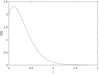
![Figure 3.2: A partial recreation of Hughes and Liberles [53] ‘Fig. 7’ showing theirapproximation to the mean rate of pseudogenization λZtwith Z„ Unip2, 16q,uc “ 1, ur “ 0.5.](https://thumb-us.123doks.com/thumbv2/123dok_us/8402157.325844/69.595.132.518.218.514/figure-recreation-hughes-liberles-showing-theirapproximation-pseudogenization-lztwith.webp)
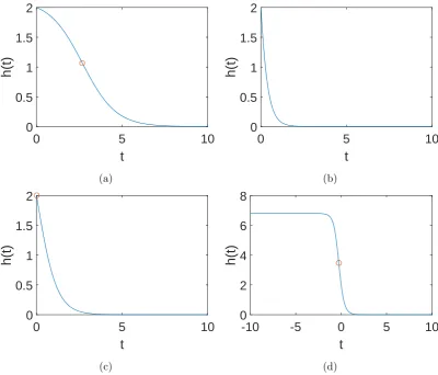
![Figure 3.7: The approximation in Konrad et al. [66] with shape parameter c “ 1. Theremaining parameters were f “ b “ 1, d “ 0.](https://thumb-us.123doks.com/thumbv2/123dok_us/8402157.325844/84.595.79.473.130.430/figure-approximation-konrad-et-shape-parameter-theremaining-parameters.webp)
![Figure 3.8: The approximation in Konrad et al. [66] with shape parameter c “ 3. The](https://thumb-us.123doks.com/thumbv2/123dok_us/8402157.325844/85.595.124.520.129.429/figure-approximation-konrad-et-al-shape-parameter-c.webp)
![Figure 3.9: The approximation in Konrad et al. [66] with shape parameter cThe remaining parameters were “ 0.5](https://thumb-us.123doks.com/thumbv2/123dok_us/8402157.325844/86.595.80.474.129.428/figure-approximation-konrad-shape-parameter-cthe-remaining-parameters.webp)