A mobile ground-based radar sensor for detection and tracking of moving objects

(1)

R E S E A R C H

Open Access

A mobile ground-based radar sensor for

detection and tracking of moving objects

Damien Vivet

1*

, Paul Checchin

1

, Roland Chapuis

1

, Patrice Faure

2

, Raphaël Rouveure

2

and Marie-Odile Monod

2

Abstract

The detection and tracking of moving objects (DATMO) in an outdoor environment from a mobile robot are difficult tasks because of the wide variety of dynamic objects. A reliable discrimination of mobile and static detections without any prior knowledge is often conditioned by a good position estimation obtained using Global Positionning System/Differential Global Positioning System (GPS/DGPS), proprioceptive sensors, inertial sensors or even the use of Simultaneous Localization and Mapping (SLAM) algorithms. In this article a solution of the DATMO problem is presented to perform this task using only a microwave radar sensor. Indeed, this sensor provides images of the environment from which Doppler information can be extracted and interpreted in order to obtain not only velocities of detected objects but also the robot’s own velocity.

Keywords:radar sensor, detection, tracking, moving objects

1 Introduction

The detection and tracking of moving objects (DATMO) are among the most challenging problems concerning autonomous driving in a dynamic environ-ment. Although the DATMO problem has been exten-sively studied for decades [1-6], it is still very difficult to accomplish these tasks from a ground vehicle at high speeds in outdoor environments.

Indeed, the most difficult issue is to separate moving objects from stationary objects. A classical approach in indoor environments is to use appearance-based or fea-ture-based techniques with cameras and laser [7-9]. Both methods rely on prior knowledge of the targets. In an outdoor context, there are many types of mobile objects such as pedestrians, animals, vehicles of different sizes (cars, trucks, etc.), which are all very difficult to detect and identify.

Furthermore, in an outdoor environment DATMO is more complex under various climatic constraints. In this context, classical sensors are limited due to the technol-ogies used: ultrasound is perturbed by wind, optical sen-sors (laser, vision) by rain, fog or the presence of dust or by poor lighting conditions. One of the particularities

of this work is the use of a microwave radar sensor. In our case, the information from this sensor regarding the signal power reflected by the targets with a 360° per sec-ond rotating antenna and a range from 5 to 100 m is used. The long range and the robustness of radar waves to atmospheric conditions make this sensor well suited for extended outdoor SLAM and DATMO applications.

In classical detection and tracking approach, multiple detections of a same object have to be done in order to obtain target velocity. Each potential moving object is tracked and its model representing both position and speed is initialized and updated. In such a method, the large number of false tracks launched, combined with incorrect data association lead to algorithm failures. In this article, based on the radar frequency modulation principle, the sensor is able to provide two simultaneous images of the environment from which Doppler infor-mation can be extracted. Also, both the distance and velocity of the targets can be estimated simultaneously. It allows to create and initialize tracks at the first detec-tion reducing following false data associadetec-tion.

In Section 2 a review of articles related to our research work is carried out. Section 3 briefly presents the microwave radar scanner developed by a Cemagref Institute team working on environmental sciences and technologies. Section 5 gives the principle used in this article in order to estimate the robot’s own velocity.

* Correspondence: [email protected]

1

Clermont Université, Université Blaise Pascal, LASMEA, UMR 6602, CNRS, Aubiere 63177, France

Full list of author information is available at the end of the article

(2)

Sections 6 and 7 present, respectively the DATMO. Finally Section 8 shows experimental results of this work. Section 9 concludes.

2 Related work

In most applications, in order to accomplish DATMO from a mobile platform, an accurate localization systems are essential [10,11]. Unfortunately, inertial measure-ment system is often very expensive and Global Posi-tionning System (GPS) or Differential Global Positioning System (DGPS) often fail in an urban or covered envir-onment such as forests because of the canyon effect. In the past decade, the simultaneous localization and map-ping (SLAM) problem has been intensively studied in robotics because it can provide an accurate estimate of the robot position without expensive inertial sensors or GPS and it allows to build consistent map of the sur-roundings without prior knowledge. For a broad and quick review of the different approaches developed to address this problem, the reader can consult the follow-ing articles [12-15].

Most of the existing SLAM methods assume that the environment is static. If there is a moving object, and the data is erroneously associated with a landmark in the map database, many localization algorithms will fail, and the map will be deteriorated by the data of the moving object. The key point to solve this problem is to isolate the data of moving and static objects. Wang pre-sented an approach to tackle SLAM and DATMO pro-blems and proved that both propro-blems are mutually beneficial [15]. These two research areas are studied jointly under the denotation SLAM and Moving Object Tracking (SLAMMOT).

In order to deal with dynamic objects, Hahnel et al. [16] filtered out moving people, and created a difference map between consecutive laser scans to remove those static but people-like objects. An implicit assumption here is that dynamic objects move all the time during their measurements. However this is not normally true. Wang [15] did on-line calculations of an occupancy map, and detected the objects that entered an object-free space. More recently, Xie et al. [17], developed a SLAMMOT application based on probabilistic occu-pancy grids.

In order to perform outdoor SLAM or SLAMMOT, laser sensors are widely used [15-20]. Research work will continue to use them due to the success story of the Velodyne HDL-64 3D LIDAR [21]. Visual sensors are also used to solve SLAMMOT problems. Ess et al. [22] presented an approach of multiperson tracking using a stereo rig mounted on a mobile platform. Solà et al. [23] described a system based on a framework called BiCamSLAM, that combines the advantages of monocular reconstruction with the advantages of

stereo vision. Marzorati et al. [24] showed that the problem of SLAMMOT can be solved with a single camera.

In the naval field [25], the use of radar sensor for SLAM(MOT) application is self-evident but in ground mobile robotics few works use such a kind of sensor. In [26], we described a trajectory-oriented SLAM. It is based on radar information over important distances using Fourier-Mellin transform for scan matching con-sidering a static environment. Radar is an interesting sensor because not only range and bearing can be obtained but also Doppler information can be used to extract velocities. This Doppler information allows to relax the assumption of static environment and to extend Radar SLAM to a SLAMMOT algorithm. In clas-sical applications, successive acquisitions are compared knowing the localization (or computing it) in order to have an idea of the movements in the surroundings of the vehicle. In our proposition, as Doppler information is measured, we do not have to wait for two successive observations to obtain detection velocities. As a result, the estimation of ego-motion from different sensor acquisitions or proprioceptive sensors is not needed. In our case, the DATMO problem can be solved without SLAM information considering moving objects in the radar frame due to the fact that Doppler is measured directly. In this article a DATMO algorithm based on Doppler information is described using the IMPALA radar sensor.

3 The IMPALA radar

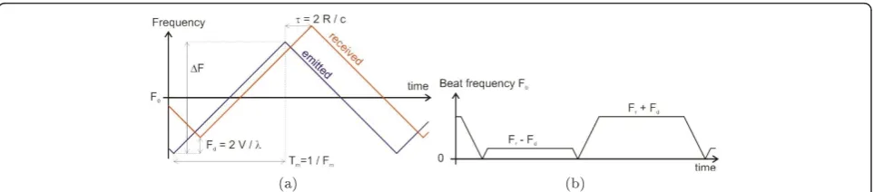
The IMPALA radar was developed by the Cemagref Institute in Clermont-Ferrand, France, for applications in the environmental monitoring domain and robotics. It is a Linear Frequency Modulated Continuous Wave (LFMCW) radar [27]. The principle of a LFMCW radar consists in transmitting a continuous frequency modu-lated signal, and measuring the frequency difference (called beat frequency Fb) between the transmitted and

the received signals. One can show thatFbcan be

writ-ten as:

Fb=

4FFmR

c

Fr

+ 2V

λ

Fd

(1)

where ΔFis the frequency excursion, Fmthe

modula-tion frequency,cthe light velocity, lthe wavelength,R

the radar-target distance (R <Rmax) and V the radial velocity of the target. The first partFr of Equation (1)

only depends on the range R, and the second partFdis

the Doppler frequency introduced by the radial velocity

(3)

1a). Considering the modulation slope, the shift intro-duced by the Doppler effect is added (negative slope) or subtracted (positive slope). Thus the sum and the differ-ence of Fb allow to determine without ambiguity the

distance and velocity of the target (see Figure 1b). An example of radar power spectra obtained with the IMPALA radar is presented in Figure 2. Four targets are detected within the radar beam: three stationary targets and a moving one. This figure illustrates a well known problem of LFMCW radar: under certain conditions, the frequency matching step may lead to target mismatch-ing, and thus may result in the creation of ghost targets [28]. One objective of the tracking step is to identify and eliminate these ghost targets.

3.1 Range resolution

Considering a zero radial velocity, the radar-target range is easily estimated from (1) with

R=Fb

c

4FFm (2)

The range resolution δR is obtained by substituting the beat frequencyFbby the frequency resolutionδFb:

δR=δFb

c

4FFm (3)

Considering a triangular modulation of duration Tm, δFbcan be expressed as

δFb=

2

Tm

= 2Fm (4)

(the signal is observed twice during the modulation period, up-slope and down-slope). Substituting (4) into (3), the well-known relationship between the signal bandwidth and the range resolution is obtained:

δR= c

2F (5)

This expression of the range resolution is a theoretical relationship, it assumes a perfect linear modulation of the transmitted signal.

3.2 Velocity resolution

Two spectra are computed within the triangular fre-quency modulation: one for the up-slope part of the modulation, the other one for the down-slope part. The radial velocity of a target is computed by measuring the frequency shift δFbetween the corresponding peaks in the up and down spectra (see mark D in Figure 2).δFis expressed as:

δF= 2Fd=

4V

λ (6)

Figure 1Triangular modulation function.(a)The time delayτis the time of flight between the radar and the target. The vertical shift is the Doppler frequency introduced by the radial velocity.(b)Frequency difference between transmitted and received signals. The sum and the difference ofFballow to estimate the distanceRand the radial velocityVof the target.

(4)

The velocity resolution δVcorresponds to the mini-mum value ofδF:

min(δF) = Fs

N (7)

with Fsthe sampling frequency and Nthe number of

frequency points. Substituting (7) into (6), the expres-sion of the velocity resolution is obtained:

δV= λFs

4N (8)

3.3 IMPALA radar characteristics

The IMPALA radar is panoramic. It is a monostatic radar, i.e., a common antenna is used for both transmit-ting and receiving. The rotatransmit-ting antenna achieves a complete 360° scan around the vehicle in 1 s, and a sig-nal acquisition is realized at each degree. The maximum range of the radar is 100 m. The radar includes micro-wave components, electronic devices for emission and reception, data acquisition and signal processing unit (see Figure 3b). An example of radar image is presented in Figure 4. The radar is positioned at the center of the image (red cross). The gray scale level indicates the amplitude of the backscattered signal. Each element of the image is positioned through its polar coordinates (d, θ). Data acquisition and signal processing units are based on an embedded Pentium Dual Core 1.6 GHz PC/104 processor. Computed data is transmitted using an Ethernet link for visualization and further processing. Main characteristics of the radar are described in Table 1.

4 Issues of DATMO using a mobile ground-based radar sensor

In order to tackle the DATMO problem with our ground-based radar sensor, different problems have to be analyzed and solved. Before detecting moving objects and estimating their speed, the Doppler effect created by the vehicle’s own velocity has to be estimated. In this

step, the Doppler disturbance created by the vehicle itself has to be removed from the radar data. Next, in order to extract non coherent entities, both corrected images obtained from the up and down modulations are compared. Differences between the scans indicate poten-tial moving objects. As the radar is subjected to impor-tant noises detected as differences between up and down images, false detections occur and have to be fil-tered out. Once moving objects are detected, a tracking process can be launched. Each moving object detection is compared and associated to the list of existing moving objects in order to update or create a new track. The approach that is used here is based on a classical Kal-man process. The choice of KalKal-man filter does not affect the reliability of our solution, even though we are aware that better alternatives could be used, especially when dealing with the problem of data association [2,29,30]. But our goal in this article was to focus our study on the behavior of a DATMO algorithm based on the Dop-pler information in a ground-based radar environment, using a well-known filter to make correct conclusions.

In the remaining part of this article we detail the pro-cess of vehicule’s own velocity estimation (cf. Section 5). In Section 6, extraction and filtering steps of

non-Figure 3 Vehicle and sensor.(a)LASMEA lab’s experimental vehicle: Vélac.(b)General view of the IMPALA radar. Overall dimensions: 24 × 27 × 30 cm (L×l×H).

Figure 4Example of a panoramic radar image. The radar is positioned at the center of the image (red cross).

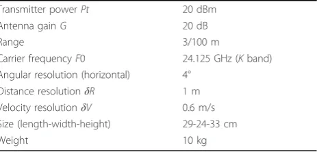
Table 1 Characteristics of the IMPALA radar

Transmitter powerPt 20 dBm

Antenna gainG 20 dB

Range 3/100 m

Carrier frequencyF0 24.125 GHz (Kband)

Angular resolution (horizontal) 4°

Distance resolutionδR 1 m

Velocity resolutionδV 0.6 m/s

Size (length-width-height) 29-24-33 cm

(5)

coherent entities considered as mobile objects are explained. Finally Section 7 presents the tracking metho-dology and all the experimental results are discussed in Section 8.

5 Robot velocity estimation

The Doppler effect is the frequency shift between the emitted and received signals when the distance between emitter and receiver is modified during the acquisition time. It is easy to demonstrate that for an emitter (or receiver) moving at velocity Vin the direction of the receiver (emitter respectively), emitting at frequency F, the frequency modification Fdis given by (1). In case

the movement is not in the direction of the receiver, radial velocity has to be considered, so:

Fd= 2×

V×cos(θ)

λ with θ ∈[0, 2π]

By measuring thisFd for different directionsθ, radial

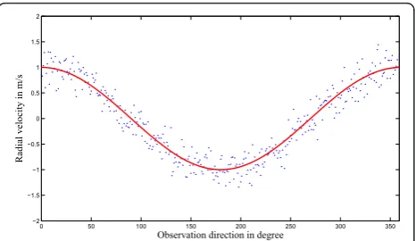
velocity can be estimated. It is reminded that Doppler effect is produced from the vehicle’s own displacement and also from the moving objects in the surroundings. In order to extract the robot’s own velocity, we use the global coherence of the surroundings. The required assumption is that more than 50% of the environment is static. For each radar beam, both the up and down modulations are compared in order to extract the Dop-pler shift using a correlation of each spectrum. From this shift, radial velocity is obtained for each ray of the observation. As radial velocity is a projection of global velocity in each observed direction, velocity profile looks like a cosine function from which parameters have to be estimated.

VDoppler=V(t)×cos(θ)

V(t) is the velocity of the radar bearing robot during the panoramic acquisition. Let us denote the robot’s velocity profileV(t) with a polynomial function of the timet:

V(t) =X(1)×tm+X(2)×tm−1+· · ·+X(m+ 1)

⎡ ⎢ ⎣

VDoppler 1

.. .

VDopplern

⎤ ⎥

⎦=tm. . .1X◦

⎡ ⎢ ⎣

cos(θ1)

.. . cos(θn)

⎤ ⎥

⎦ (9)

where○is the Hadamard product function.

Median least square algorithm [31] is applied to esti-mate the parameters of Xof the functionV(t) based on Doppler estimates for each radar beam. This principle is illustrated in Figure 5.

Each measurement of Doppler velocityVDoppler ihas an uncertaintysDoppler. As a result, parameters of X of

the function V(t) are estimated with their own uncer-tainty. Vehicle’s own velocity profile V(t) and uncer-taintysV(t)can be known during the radar acquisition.

6 Search of non coherent entities

A Doppler image representing the Doppler effect cre-ated by the vehicle is obtained based on the previous estimated robot’s velocity profile and (9). This result is presented in Figure 6.

If no mobile object is present in the scan, no differ-ence of velocity should be detected. In order to correct radar images, each power spectrumSupand Sdwof the up and down acquisitions is modified based on the expected Doppler effectΔfiin the observed directionθi

to obtain the corrected dataScupand Scdw.

Scup_θ_i(fc) =Sup_θ_i(f −fi) Scdwθi(fc) =Sdwθi(f −fi)

0 50 100 150 200 250 300 350

−2

−1.5

−1

−0.5 0 0.5 1 1.5 2

Observation direction in degree

Radial velocity in m/s

Figure 5 Doppler velocity profile estimation during the

acquisition.

(6)

Corrected images and spectrum comparison allow to extract the area not conforming to the Doppler profile. The differenceis given by:

ε= Scup_θ_1:_n(fc)−Scdwθ1:n(fc)

In each area, entities are extracted with a local descriptor created from original up and down radar images. Examples of local descriptors are given in Figure 7. The correlation score in the depth direction (direction where the Doppler effect is visible) gives the global coherence of the extracted object and so its own Dop-pler velocity.

As radar is subjected to important noises detected as differences between up and down images, false detec-tions occur. A correlation score is used in order to filter some of false detections. Other false detections will be filtered out by the temporal moving object tracking pro-cess and the probabilistic approach (see Section 7).

In order to characterize the detections, a probabilistic study of this moving object detector has been done. As radar response varies as a function of the distance, the probabilities of correct and false detection knowing the presence of mobile objects have been computed as a function of the distance and are presented in Figure 8. The experiment was conducted in a complex and uncontrolled environment. Only known mobile objects were considered as good detections whereas pedestrians

or uncontrolled parasite vehicles were treated as noise. As a consequence the probabilistic study is a pessimistic evaluation.

In order to explain these true positive (TP) and false negative (FN) rates, radar and Doppler characteristics need to be considered. Doppler represents the radial velocity of objects. When an object is moving perpendi-cularly to the sensor, Doppler is null and so there is no detection. This explains the 20% FN rates at low range. Moreover, because of radar signal properties, detections at a high range are less powerful and much more noised than detections at a short distance. So the longer the range of the detection is, the lower the TP rates of mov-ing object detection are.

At the end of this detection step, each potential mov-ing object detected (notedO) is initialized as follows:O

= [Xo, Vo, po] where Xo = (xo,yo) is the position of the

object in the radar frame,Vo= (Vox,Voy)is the object’s

velocities and po is the probability of being a mobile

object. This probability is obtained based on the detec-tor characterization and varies according to the distance from the radar.

7 Tracking of moving objects

Each moving object detection is compared and asso-ciated to the list of existing moving objects in order to update or create a new track. This Detection association is based on the classical Mahalanobis distance taking into account both position and Doppler measurement along with their uncertainties. For each potential mobile object, tracking is done with a classical Kalman approach based on a constant velocity model. Other tracking methods using Interacting Multiple Model (IMM) and Multiple Hypothesis Tracking (MHT) tech-niques could be used to refine detection and data asso-ciation [3]. Additional difficulty with radar sensor is the absence of shape information.

At each detection and association step, position and velocity of moving objects are estimated by the Kalman process and a concurrent process updates the probabil-ity of each track according to the detection or not of the moving object (see (10) and (11), respectively). Pos-terior probability p(O|d) and p(O|¯d)are processed as follows:

p(O|d) = p(O)p(d|O)

p(d|O)p(O) +p(d| ¯O))(1−p(O)) (10)

p(O|¯d) = p(O)p(d¯|O)

p(d¯|O)p(O) + (1−p(d| ¯O)(1−p(O)) (11)

with p(O) the prior probability of the track, p(d|O) and p(d¯|O) the TP and FN rates of the detector

Frequency indices

Angle indices

Up modulation

0 20 40 60

−10 0 10 20 Frequency indices Angle indices Down modulation

0 20 40 60

−10 0 10 20 Frequency indices Angle indices Up modulation

0 20 40 60

−10 0 10 20 Frequency indices Angle indices Down modulation

0 20 40 60

−10

0

10

20

Figure 7Local polar descriptor of entities detected as moving

(7)

respectively. These rates are linked to the distance of the detected object (cf. Figure 8). Then posterior probability

p(O|d) or(p(O|¯d))becomes the new object existence probabilityp(O).

Track management is done based on different criteria: in case of out of range moving objects (> 100 m) or low probability of existence (po< 0.05).

8 Experimental results

For these experiments, two experimental vehicles have been used. One was equipped with proprioceptive sen-sors, D-GPS for ground truth estimation and IMPALA FMCW panoramic radar imager. The other one called Vélac acts as the target (cf. Figure 3), and was equipped with proprioceptive sensors and D-GPS as well to have ground truth for moving object detection and tracking. Experiments were conducted in Clermont-Ferrand, France, on Blaise Pascal University campus, at variable speeds (with maximum 30 km/h).

8.1 Robot’s own velocity estimation

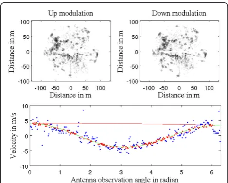
As a first step, the robot’s own velocity has been esti-mated with different data sets acquired from the IMPALA radar sensor. Ground truth for velocity was taken from odometer and D-GPS. Speed estimation has been done on different kinds of displacements, i.e., recti-linear displacement and also classical road traffic displa-cement with different curves. Results of velocity profile extraction based on the method described in Section 5 are presented in Figure 9: on top, the two radar images obtained with the up and down modulation. For each acquired radar beam, velocity is estimated (in blue dots) based on correlation techniques. The median least square method using covariance of the extracted

Doppler is used to select inliers Doppler detection (in red dots) and to process the robot’s velocity profile dur-ing the acquisition (in red line). The Doppler velocity profile is estimated in green line.

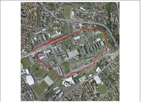
The robot’s velocity obtained during a 10 min, 2 km, travel is presented in Figure 10. Maximum speed during this travel was approximately 30 km/h. Trajectory is presented on aerial image in Figure 11. Ground truth for velocity is taken from filtered odometer data and DGPS. The acquisition system encountered a problem at the end of the experiment, so no reference is available for the last few meters.

Doppler velocity estimation with correlation presents a standard deviation of 0.3 m/s which corresponds to the correlation resolution. The estimated speed with its respective uncertainty is presented in Figure 10. A sta-tistical evaluation of our Doppler odometry has been done. The linear velocity estimate errorV has a

stan-dard deviation σεV = 0.76 m/s and a mean εV= 0.27 m/s. An error during the classical odometer recording occurred at the end of the trajectory, which explains the 0 values on the red data while Doppler is still estimating the velocity.

8.2 Detection and tracking of moving objects

Different experiments have been conducted with a GPS referenced vehicle in complex and noisy environment resulting in several false detections. During this experi-ment, the vehicle equipped with the radar is static. Each potential mobile object is tracked and updated based on Doppler observations. The evolution of the existence probability of each detection and their respective

0 10 20 30 40 50 60 70 80 90 100

0 0.1 0.2 0.3 0.4 0.5 0.6 0.7 0.8 0.9 1

Distance in meter

Probability

True positives rate False negatives rate

Figure 8 Rate of TP and FN detections as a function of the

range. Figure 9Robot’s velocity profile estimation step: top left, up

radar image, top right, down radar image. Bottom, extracted

(8)

trajectories are presented in Figures 12 and 13. Among the false detections, we can observe that their probabilities decrease quickly and then their tracks are deleted. Real mobile objects are tracked for a longer time and their probability increases at each new detection. We can see two moving objects in the data: one at timet= 25 to 50 represented in red, the other one at timet= 58 to 78 in blue. Respective trajectories are represented in Figure 13. Each track is plotted with the same color used in Figure 12. The trajectories of the two real moving objects are the two vertical straight lines. The accuracy of these tracks,

both on position and velocity, has been processed based on D-GPS and proprioceptive sensor ground truth. The longest track (in red in Figure 12) is analyzed in Figure 14. The tracking error of the moving object has a mean of 4 m in position and a mean error of 0.3 m/s in velocity.

Trajectories presented in Figure 13 represent all the launched tracks. Two of them are due to real moving objects, while the remaining tracks are due to noises. Nevertheless, even if noise is important, their probability of existence is always decreasing and after five acquisi-tions (indeed 5 s) the majority of them are deleted as

0 100 200 300 400 500 600

−1 0 1 2 3 4 5 6 7 8

Time in seconde

Linear velocity in m/s

Figure 10Robot’s velocity profile estimation during the entire acquisition based on Doppler effect analysis. In red, ground truth velocity is obtained with filtered odometer data. In blue the estimates given by the method with the associated 1suncertainty in green.

(9)

considered disturbances, while the remaining are con-firmed as real mobile objects.

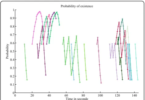
Tracking of multiple objects has been done in differ-ent formations (cf. Figure 15): with vehicles in a convoy and also with vehicles crossing one another near the radar sensor. A total of four vehicles moved in the sur-roundings of the IMPALA sensor at various speeds. In the presented experiment, a convoy of three vehicles started from time 20 to 30 s (cf. Figure 16a,c,e) and crossed a vehicle coming from the opposite direction at time 55 s (cf. Figure 17a). Then the three vehicles returned from time 110 to 140 s (Figure 17c,e,g). Trajec-tories and probabilities of moving objects from the first part of the experiment are given in Figure 16. Results concerning the vehicles coming from the opposite direc-tion are presented in Figure 17. For each mobile object, a discontinuity in the track is observed due to (1) its proximity to the radar sensor and (2) to the fact that the Doppler effect of the mobile object becomes too

0 10 20 30 40 50 60 70 80 90

0 0.1 0.2 0.3 0.4 0.5 0.6 0.7 0.8 0.9 1

Time in second

Probability

Mobile objects probabilities

Figure 12 Evolution of moving object tracks and of their

existence probability: each track has got a different color.

−100 −80 −60 −40 −20 0 20 40 60 80 100

−100

−80

−60

−40

−20 0 20 40 60 80 100

Distance in meter

j j

Figure 13Trajectory of moving objects: each track has got a different color, the green hashed line is the reference

trajectory. In red dot the radar position.

0 5 10 15 20 25

−10

−5 0 5 10

Time in second

Distance in mete

r

0 5 10 15 20 25

−10

−5 0 5 10

Time in second

Distance in meter

0 5 10 15 20 25

−10

−5 0 5 10

Time in second

Distance in meter

0 5 10 15 20 25

−10 0 10

Time in second

Velocity in m/s

0 5 10 15 20 25

−10 0 10

Time in second

Velocity in m/s

0 5 10 15 20 25

−10 0 10

Time in second

Velocity in m/s

Figure 14Localization and velocity evaluations.(a)Localization and(b)velocity errors of the D-GPS referenced moving object. From top to bottom error on(a)x, y and distance(b)x velocity, y velocity and linear velocity with their 3_sbound.

(10)

small to be detected (as a function of radial velocity). This explains as to why two different tracks are initia-lized for the same mobile object.

All trajectories and all probabilities including false tracks and detection are super-imposed in Figures 18 and 19.

(11)

9 Conclusion

A method based on Doppler measurements for com-puting position and instantaneous velocity of moving objects in the surroundings of a robot using an original

(12)

extraction and processing of landmarks remain a chal-lenge because of detection ambiguity, false detection, Doppler Speckle effect and the absence of detection descriptors. Moreover, the data is affected by the Dop-pler effect created by the vehicle’s own velocity. Cor-rection based on a Doppler velocimetry has been applied in order to globally correct radar data. Once data is free from radar movement disturbances, non-coherent radar echoes are extracted and supposed as new moving objects. The probabilistic evaluation of our detector has been done and used to confirm or invalidate launched tracks at each new detection. Tracking of each entity is based on a classical extended

Kalman filter. This approach was evaluated on real radar data, first, showing exteroceptive Doppler veloci-metry feasibility and reliability at high speed (≈ 30 km/ h), then detecting a D-GPS referenced moving object in a very noisy environment. A comparison between radar DATMO results and ground truth has been done. The main novelties of the proposed approach are the use of a panoramic LFMCW radar sensor and Doppler information for a ground mobile robotic application for DATMO purpose. Future work will include improving our radar SLAM (SLAM) process [26] by adding consideration of distortion due to non instantaneous data acquisition, Doppler information, and, as a consequence, a DATMO algorithm to tackle radar SLAMMOT problems in an extended outdoor environment. Moreover implementation of other filter techniques such as GM-CPHD (Gaussian mixture car-dinalized probability hypothesis density) [32] will be compared with the actual Kalman method.

Acknowledgements

This study was supported by the Agence Nationale de la Recherche (ANR_– the French national research agency) (ANR Impala PsiRob– ANR-06-ROBO-0012).

Author details

1

Clermont Université, Université Blaise Pascal, LASMEA, UMR 6602, CNRS, Aubiere 63177, France2_{Cemagref, Technologies and Information Systems}

Research Unit, Aubiere 63172, France

Competing interests

The authors declare that they have no competing interests.

Received: 14 May 2011 Accepted: 23 February 2012 Published: 23 February 2012

References

1. Y Bar-Shalom, Tracking methods in a multitarget environment. IEEE Trans Automat Control.23, 4 (1978)

2. Y Bar-Shalom, XR Li,Multitarget-Multisensor Tracking: Principles and Techniques, (YBS, Dan-vers, MA, 1995)

3. S Blackman, R Popoli,Design and Analysis of Modern Tracking Systems, (Artech House, MA, 1999)

4. H Blom, Y Bar-Shalom, The interacting multiple model algorithm for systems with Markovian switching coefficients. IEEE Trans Automat Control. 33(8), 780–783 (1988). doi:10.1109/9.1299

5. DB Reid, An algorithm for tracking multiple targets. IEEE Trans Automat Control.24(6), 843_–854 (1979). doi:10.1109/TAC.1979.1102177

6. D Schulz, W Burgard, D Fox, AB Cremers, Tracking multiple moving targets with a mobile robot using particle filters and statistical data association, in IEEE Int Conf on Robotics and Automation, Seoul, Korea, pp. 1665–70 (21-26 May 2001)

7. B Kluge, C Kohler, E Prassler, Fast and robust tracking of multiple objects with a laser range finder, inIEEE Int Conf on Robotics and Automation, Seoul, Korea, pp. 1683–88 (21-26 May 2001)

8. M Lindstrom, JO Eklundh, Detecting and tracking moving objects from a mobile platform using a laser range scanner, inProc Int Conf On Intelligent Robots and Systems, Maui, HI, USA, pp. 1364–69 (2001)

9. S Gidel, P Checchin, C Blanc, T Chateau, L Trassoudaine, Pedestrian detection and tracking in an urban environment using a multilayer laser scanner. IEEE Trans Intell Trans Syst.11(3), 579_–588 (2010)

10. E Prassler, J Scholz, P Fiorini, A Robotic Wheelchair for crowded public environments. Robot Automat Mag.8, 38–45 (2001). doi:10.1109/100.924358 Figure 18Trajectories of all moving objects detected: each

track has got a different color, the green hashed line is the

reference trajectory. In red dot the radar position.

0 20 40 60 80 100 120 140

0 0.1 0.2 0.3 0.4 0.5 0.6 0.7 0.8 0.9

1 Probability of existence

Time in seconde

Probability

Figure 19Evolution of all moving object tracks and of their

(13)

11. L Zhao, C Thorpe, Qualitative and quantitative car tracking from a range image sequence, inIEEE Conf on Computer Vision and Pattern Recognition, Santa Barbara, CA, USA, pp. 496–501 (1998)

12. T Bailey, H Durrant-Whyte, Simultaneous localization and mapping: part II_– state of the art. Robot Aut Mag.13, 108–117 (2006)

13. G Dissanayake, P Newman, H Durrant-Whyte, S Clark, M Csobra, A solution to the simultaneous localization and map building problem. IEEE Trans Robot Autom.17(3), 229_–241 (2001). doi:10.1109/70.938381

14. H Durrant-Whyte, T Bailey, Simultaneous localization and mapping: part I– the essential algorithms. Robot Autom Mag.9, 99–108 (2006)

15. CC Wang, Simultaneous Localization, Mapping and Moving Object Tracking, Ph.D. thesis, (Carnegie Mellon Univ, 2004)

16. D Hahnel, W Burgard, D Fox, S Thrun, An efficient FastSLAM algorithm for generating maps of large-scale cyclic environments from raw laser range measurements, inProc Conf on Intelligent Robots and Systems, 2003, Las Vegas, USA, pp. 206–211. (2003)

17. J Xie, F Nashashibi, M Parent, O Garcia Favrot, A real-time robust SLAM for large-scale outdoor environments, in17th ITS World Congress(2010) 18. P Pfaff, R Triebel, C Stachniss, P Lamon, W Burgard, R Siegwart, Towards

mapping of cities, inProc of the IEEE Int Conf on Robotics and Automation (ICRA), Rome, Italy, pp. 4807–4813 (Apr 2007)

19. A Howard, D Wolf, G Sukhatme, Towards 3D mapping in large urban environments, inProc IEEE/RSJ Int Conf on Intelligent Robots and Systems (IROS), Sendai, Japan, pp. 419_–424 (Sep 2004)

20. M Bosse, R Zlot, Map matching and data association for large-scale two-dimensional laser scan-based SLAM. Int J Robot Res.27, 667_–691 (2008). doi:10.1177/0278364908091366

21. J Leonard, J How, S Teller, M Berger, S Campbell, G Fiore, L Fletcher, E Frazzoli, A Huang, S Karaman, O Koch, Y Kuwata, D Moore, E Olson, S Peters, J Teo, R Truax, M Walter, D Barrett, A Epstein, K Maheloni, K Moyer, T Jones, R Buckley, M Antone, R Galejs, S Krishnamurthy, J Williams, A Perception Driven Autonomous Urban Vehicle. J Field Robot.25(10), 727_–774 (2008). doi:10.1002/rob.20262

22. A Ess, B Leibe, K Schindler, LV Gool, Robust multi-person tracking from a mobile platform. IEEE Trans Pattern Anal Mac Intell.31(10), 1831_–1846 (2009)

23. J Solà, A Monin, M Devy, Bicamslam: Two times mono is more a than stereo, inProc of the IEEE Int Conf on Robotics and Automation (ICRA), Roma, Italy, pp. 4795–4800 (2007)

24. D Marzorati, M Matteucci, D Migliore, R Rigamonti, G Sorrenti, Use a single camera for simultaneous localization and mapping with mobile object tracking in dynamic environments, inICRA09 Workshop on Safe navigation in open and dynamic environments Application to autonomous vehicles, (Kobe, Japan, 2009)

25. C Bibby, I Reid, A hybrid SLAM representation for dynamic marine environments, inIEEE Int Conf on Robotics and Automation ICRA, Anchorage, Alaska, USA, pp. 257–264 (3-7 May 2010)

26. F Gérossier, P Checchin, C Blanc, R Chapuis, L Trassoudaine, Trajectory-oriented EKF-SLAM using the Fourier-Mellin transform applied to microwave radar images, inIEEE/RSJ Int Conf on Intellig Robots and Systems (IROS), St. Louis, USA, pp. 4925–4930 (2009)

27. M Skolnik,Introduction to Radar Systems, (McGraw Hill, New York, 1980) 28. M Reiher, B Yang, Derivation of the frequency mismatch probability in

linear FMCW radar based on target distribution, inIEEE RadarCon 2009, Pasadena, USA, pp. 1_–6 (2009)

29. M Ulmke, O Erdinc, P Willett, GMTI tracking via the gaussian mixture cardinalized probability hypothesis density filter. IEEE Trans Aerosp Electron Syst.46, 1821–1833 (2010)

30. R Mahler, PHD filters of higher order in target number. IEEE Trans Aerosp Electron Syst.43, 1523–1543 (2007)

31. WH Press, SA Teukolsky, WT Vetterling, BP Flannery, inNumerical Recipes 3rd Edition: The Art of Scientific Computing, 3rd edn. (Cambridge University Press, New York, 2007)

32. M Ulmke, O Erdinc, P Willett, GMTI tracking via the gaussian mixture cardinalized probability hypothesis density filter. IEEE Trans Aerosp Electron Syst.46, 1821_–1833 (2010)

doi:10.1186/1687-6180-2012-45

Cite this article as:Vivetet al.:A mobile ground-based radar sensor for

detection and tracking of moving objects.EURASIP Journal on Advances

in Signal Processing20122012:45.