Study of transient indoor temperature for a HVAC room using a modified CFD method

(1)

ScienceDirect

Available online at Available online at www.sciencedirect.comwww.sciencedirect.com

ScienceDirect

Energy Procedia 00 (2017) 000–000

www.elsevier.com/locate/procedia

Peer-review under responsibility of the Scientific Committee of The 15th International Symposium on District Heating and Cooling.

The 15th International Symposium on District Heating and Cooling

Assessing the feasibility of using the heat demand-outdoor

temperature function for a long-term district heat demand forecast

I. Andri

ć

a,b,c

_{*, A. Pina}

a

_{, P. Ferrão}

a

_{, J. Fournier}

b

_{., B. Lacarrière}

c

_{, O. Le Corre}

c a_{IN+ Center for Innovation, Technology and Policy Research - Instituto Superior Técnico, Av. Rovisco Pais 1, 1049-001 Lisbon, Portugal}

b_{Veolia Recherche & Innovation, 291 Avenue Dreyfous Daniel, 78520 Limay, France}

c_{Département Systèmes Énergétiques et Environnement - IMT Atlantique, 4 rue Alfred Kastler, 44300 Nantes, France}

Abstract

District heating networks are commonly addressed in the literature as one of the most effective solutions for decreasing the greenhouse gas emissions from the building sector. These systems require high investments which are returned through the heat sales. Due to the changed climate conditions and building renovation policies, heat demand in the future could decrease, prolonging the investment return period.

The main scope of this paper is to assess the feasibility of using the heat demand – outdoor temperature function for heat demand forecast. The district of Alvalade, located in Lisbon (Portugal), was used as a case study. The district is consisted of 665 buildings that vary in both construction period and typology. Three weather scenarios (low, medium, high) and three district renovation scenarios were developed (shallow, intermediate, deep). To estimate the error, obtained heat demand values were compared with results from a dynamic heat demand model, previously developed and validated by the authors.

The results showed that when only weather change is considered, the margin of error could be acceptable for some applications (the error in annual demand was lower than 20% for all weather scenarios considered). However, after introducing renovation scenarios, the error value increased up to 59.5% (depending on the weather and renovation scenarios combination considered). The value of slope coefficient increased on average within the range of 3.8% up to 8% per decade, that corresponds to the decrease in the number of heating hours of 22-139h during the heating season (depending on the combination of weather and renovation scenarios considered). On the other hand, function intercept increased for 7.8-12.7% per decade (depending on the coupled scenarios). The values suggested could be used to modify the function parameters for the scenarios considered, and improve the accuracy of heat demand estimations.

Peer-review under responsibility of the Scientific Committee of The 15th International Symposium on District Heating and Cooling.

Keywords:Heat demand; Forecast; Climate change

This is an open access article under the CC BY-NC-ND license (https://creativecommons.org/licenses/by-nc-nd/4.0/)

Selection and peer-review under responsibility of the scientific committee of the 2nd International Conference on Energy and Power, ICEP2018. 10.1016/j.egypro.2019.02.176

10.1016/j.egypro.2019.02.176

Selection and peer-review under responsibility of the scientific committee of the 2nd International Conference on Energy and Power, ICEP2018.

1876-6102 Available online at www.sciencedirect.com

ScienceDirect

2nd International Conference on Energy and Power, ICEP2018, 13–15 December 2018,

Sydney, Australia

Study of transient indoor temperature for a HVAC room using a

modified CFD method

Lu Zhang

a

_{, Xiaoling Yu}

a*

_{, Qian Lv}

a

_{, Feng Cao}

a

_{, Xiaolin Wang}

a,b_*

a_{School of Energy and Power Engineering, Xi’an Jiaotong University, Xi’an, 710049, China.} b_{School of Engineering, University of Tasmania, Hobart, TAS 7001, Australia.}

Abstract

The change of the transient indoor temperature is crucial to evaluate electrical power consumption of a heat pump and thermal comfort of the room. Computational Fluid Dynamics (CFD) model can provide the most comprehensive information in transient indoor temperature simulations. In CFD models, the transient flow and temperature fields are fully coupled. This coupling leads to high computation cost and time, which limits the CFD application in practice. A segregated CFD model was then proposed to speed up the computation. However, such model is not very accurate during the transient analysis. In this paper, a semi-coupled CFD model combining advantages of the fully-coupled CFD model and the segregated CFD model was proposed. In this CFD model, the flow and the temperature fields are firstly solved by fully coupled simulation during the transient start up period and then the segregated CFD is used for the transient temperature rising simulation. This method can reduce the computation time without losing the simulation accuracy. The transient indoor temperature is studied using the proposed method and the results are compared with those obtained from both fully-coupled and segregated CFD models. The hot air temperature is first calculated using a lumped-parameter method, and then it is applied as an initial boundary condition in the CFD models. The comparison results show that the proposed semi-coupled CFD model shows a promising capability of capturing the critical transient thermal responses for the air-conditioning room, and it can effectively reduce the computing time with an acceptable accuracy.

Keywords: Heat pump, Energy consumption, HVAC room, Computational fluid dynamics

* Corresponding author. Xiaoling Yu. Tel.:86-29-82664844.

E-mail address: [email protected]

Available online at www.sciencedirect.com

ScienceDirect

2nd International Conference on Energy and Power, ICEP2018, 13–15 December 2018,

Sydney, Australia

Study of transient indoor temperature for a HVAC room using a

modified CFD method

Lu Zhang

a

_{, Xiaoling Yu}

a*

_{, Qian Lv}

a

_{, Feng Cao}

a

_{, Xiaolin Wang}

a,b_*

Abstract

2 Lu Zhang / Energy Procedia 00 (2018) 000–000

1.Introduction

In recent years, clean electric heating is required to replace coal-based heating by the Chinese government to solve severe environmental problems caused by coal combustion in winter. Heat pump is a popular electric heating technology used for space heating due to its high energy conversion efficiency. However, the heat pump power consumption and the room thermal comfort are heavily affected by the room air temperature during the start-up period. Thus, it is important to study the transient room air temperature during this period.

Many researchers have applied different simulation methods to investigate the transient indoor air temperature.

Bozkır et al. [1] proposed a lumped parameter model (LPM) to study heat transfer in a room heated by finned radiators. The results were validated by experimental data. Romano et al. [2] used the LPM to simulate the indoor air temperature and humidity behavior inside a showcase under different conditions of the museum indoor air. A re-configurable freestanding showcase was experimentally tested to prove that the LPM is a useful tool for new showcase design and optimization. These researches showed that the LPM can achieve good results in a room or a small space with natural convection, but it was unsuitable for a space with forced convection since the air in the room was treated as a whole with a uniform temperature and a static state in the LPM.

Computational Fluid Dynamics (CFD) models are versatile and can provide more comprehensive information for transient indoor temperature simulations. Popovici [3] studied a Heating Ventilation and Air-Conditioning (HVAC) system in summer and winter times using ANSYS-Fluent. A two-Dimensional model was developed to investigate the indoor air temperature and air velocity under different conditions. Fang et al. [4] used the combined CFD and network model to calculate the air temperature distribution in an air-conditioned office room under four working conditions, and the model was validated using the experimental data under both steady and transient conditions. In CFD models, the velocity and the temperature fields are fully-coupled at each time step, which leads to high computational cost and time. To speed up CFD, Wang et al. [5] systematically examined coarse-grid CFD to reduce computing time within acceptable accuracy. Zuo et al. [6] used the FFD (Fast Fluid Dynamics) method with and without turbulence treatments to study systematically four basic flows in buildings, the results showed that, the FFD was less accurate than CFD, but it was 50 times faster than CFD. Wang et al. [7] proposed a discrete state-space method, called state-space fluid dynamics (SFD) to handle transient velocity and temperature fields. In SFD, the flow field was fixed, and the velocity field and turbulence viscosity was pre-calculated using CFD. Thereafter, the discretized energy conservation equations were transformed into the state-space model and solved. Great amount of computing time was saved since the momentum conservation equations did not need to be solved. In this method, the velocity fields were assumed to be segregated with the temperature fields. SFD could generally produce better results than FFD when the time step size is larger, which allowed SFD run faster than FFD. W Tian et al. [8] proposed a coupled ISAT (in situ adaptive tabulation) and FFD (fast fluid dynamics) method to solve stratified indoor airflow. In the mothed, the ISAT would retrieve the solutions from an existing data set if the estimated prediction error was within a pre-defined tolerance, otherwise, the ISAT would execute the FFD simulation. The result showed the ISAT was able to answer query points both inside and close to training domain using retrieve actions within a time less than 0.001 s for each query.

This paper proposed a semi-coupled CFD model combining advantages of the fully-coupled CFD model and the segregated CFD model. In the semi-coupled CFD model, the flow fields and the temperature fields are firstly solved by fully-coupled CFD simulation before the flow fields were developed to a steady state. At the steady flow fields, the temperature fields were only needed to be solved by an uncoupled simulation. The transient room air temperature of a HVAC bedroom was simulated using the semi-coupled CFD model, and the simulation results were compared with those obtained from the fully-coupled CFD model and the segregated CFD model.

2.The semi-coupled CFD model

2.1.Description of the HVAC room

(2)

Lu Zhang et al. / Energy Procedia 160 (2019) 420–427 421 Available online at www.sciencedirect.com

ScienceDirect

2nd International Conference on Energy and Power, ICEP2018, 13–15 December 2018,

Sydney, Australia

Study of transient indoor temperature for a HVAC room using a

modified CFD method

Lu Zhang

a

_{, Xiaoling Yu}

a*

_{, Qian Lv}

a

_{, Feng Cao}

a

_{, Xiaolin Wang}

a,b_*

Abstract

Available online at www.sciencedirect.com

ScienceDirect

2nd International Conference on Energy and Power, ICEP2018, 13–15 December 2018,

Sydney, Australia

Study of transient indoor temperature for a HVAC room using a

modified CFD method

Lu Zhang

a

_{, Xiaoling Yu}

a*

_{, Qian Lv}

a

_{, Feng Cao}

a

_{, Xiaolin Wang}

a,b_*

Abstract

1.Introduction

In recent years, clean electric heating is required to replace coal-based heating by the Chinese government to solve severe environmental problems caused by coal combustion in winter. Heat pump is a popular electric heating technology used for space heating due to its high energy conversion efficiency. However, the heat pump power consumption and the room thermal comfort are heavily affected by the room air temperature during the start-up period. Thus, it is important to study the transient room air temperature during this period.

Many researchers have applied different simulation methods to investigate the transient indoor air temperature.

Bozkır et al. [1] proposed a lumped parameter model (LPM) to study heat transfer in a room heated by finned radiators. The results were validated by experimental data. Romano et al. [2] used the LPM to simulate the indoor air temperature and humidity behavior inside a showcase under different conditions of the museum indoor air. A re-configurable freestanding showcase was experimentally tested to prove that the LPM is a useful tool for new showcase design and optimization. These researches showed that the LPM can achieve good results in a room or a small space with natural convection, but it was unsuitable for a space with forced convection since the air in the room was treated as a whole with a uniform temperature and a static state in the LPM.

Computational Fluid Dynamics (CFD) models are versatile and can provide more comprehensive information for transient indoor temperature simulations. Popovici [3] studied a Heating Ventilation and Air-Conditioning (HVAC) system in summer and winter times using ANSYS-Fluent. A two-Dimensional model was developed to investigate the indoor air temperature and air velocity under different conditions. Fang et al. [4] used the combined CFD and network model to calculate the air temperature distribution in an air-conditioned office room under four working conditions, and the model was validated using the experimental data under both steady and transient conditions. In CFD models, the velocity and the temperature fields are fully-coupled at each time step, which leads to high computational cost and time. To speed up CFD, Wang et al. [5] systematically examined coarse-grid CFD to reduce computing time within acceptable accuracy. Zuo et al. [6] used the FFD (Fast Fluid Dynamics) method with and without turbulence treatments to study systematically four basic flows in buildings, the results showed that, the FFD was less accurate than CFD, but it was 50 times faster than CFD. Wang et al. [7] proposed a discrete state-space method, called state-space fluid dynamics (SFD) to handle transient velocity and temperature fields. In SFD, the flow field was fixed, and the velocity field and turbulence viscosity was pre-calculated using CFD. Thereafter, the discretized energy conservation equations were transformed into the state-space model and solved. Great amount of computing time was saved since the momentum conservation equations did not need to be solved. In this method, the velocity fields were assumed to be segregated with the temperature fields. SFD could generally produce better results than FFD when the time step size is larger, which allowed SFD run faster than FFD. W Tian et al. [8] proposed a coupled ISAT (in situ adaptive tabulation) and FFD (fast fluid dynamics) method to solve stratified indoor airflow. In the mothed, the ISAT would retrieve the solutions from an existing data set if the estimated prediction error was within a pre-defined tolerance, otherwise, the ISAT would execute the FFD simulation. The result showed the ISAT was able to answer query points both inside and close to training domain using retrieve actions within a time less than 0.001 s for each query.

This paper proposed a semi-coupled CFD model combining advantages of the fully-coupled CFD model and the segregated CFD model. In the semi-coupled CFD model, the flow fields and the temperature fields are firstly solved by fully-coupled CFD simulation before the flow fields were developed to a steady state. At the steady flow fields, the temperature fields were only needed to be solved by an uncoupled simulation. The transient room air temperature of a HVAC bedroom was simulated using the semi-coupled CFD model, and the simulation results were compared with those obtained from the fully-coupled CFD model and the segregated CFD model.

2.The semi-coupled CFD model

2.1.Description of the HVAC room

(3)

422 Lu Zhang et al. / Energy Procedia 160 (2019) 420–427

Lu Zhang / Energy Procedia 00 (2018) 000–000 3

[image:3.544.180.365.176.311.2]

operation state. This paper aims to simulate the transient room air temperature rising from the start to steady operation of the heat pump. The air is closed and circulated in the room. It is inhaled, heated, and then blown off by the fan coil. In the model, the velocity of the hot air blown off by the fan coil is assumed to be constant, but its temperature is changed with time. It is obvious that the velocity fields are largely unsynchronized with the temperature field changes, with velocity fields changing in seconds whereas temperature changing in minutes or even longer. Thus, the flow and the temperature fields are firstly solved by the fully coupled CFD simulation during the start-up period. Then the velocity fields are fixed and the discretized energy conservation equations are transformed into the fixed velocity fields to solve the transient air temperatures.

Fig. 1. The model of a HVAC bedroom

2.2.The three-dimensional transient indoor air temperature mathematical model

The three-dimensional transient room air temperature model can be described by mass conservation equation, momentum conservation equation, and energy equation.

Mass conservation equation (continuity equation):

0 u

v

w

x

y

z

ρ

τ

∂

₊

∂

₊

∂

₊

∂

₌

∂

(1)

Where ρ is density, kg/m3_;_u_,_v_,_w_{are components of velocity vector in}_x_,_y_,_z_{direction, respectively, m/s.}

N-S equation (momentum conservation equation):

2

x

y

z

u

_u

u

_v

u

_w

u

p

_g

_u

x

y

z

x

v

_u

v

_v

v

_w

v

p

_g

_v

x

y

z

y

w

_u

w

_v

w

_w

w

p

_g

_w

x

y

z

ρ

µ

τ

ρ

µ

τ

ρ

µ

τ



∂



∂

+

= −

+

+ ∇



_∂



_∂







∂

₊

∂

₊

∂

₊

∂



_{= −}

∂

₊

_{+ ∇}



_∂



_∂







∂

₊

∂

₊

∂

₊

∂



_{= −}

∂

₊

_{+ ∇}



_∂



_∂





(2)

Where ρis pressure, Pa; u is dynamic viscosity, Pa·s; g is acceleration of gravity, m/s2_;_{𝛻𝛻𝛻𝛻}2_{is Laplacian.}

Energy equation:

p

T

c

u

v

w

S

x

y

z

x

y

z

ρ

λ

τ



∂

₊

∂

₊

∂

₊

∂



₌

∂



∂



₊

∂



∂



₊

∂



∂



₊



_∂



_∂



_

_∂

_



_∂



_∂



_∂



_

_∂



_









(3)

Where S is internal heat source of the fluid, J; λ is thermal conductivity, W/(m·K).

For the HVAC bed-room, the indoor air flow is turbulent, and k-ε model is used to deal with the turbulent flow. The equations are discretized using the first order implicit scheme. In the semi-coupled CFD model, the transient continuity equation and N-S equation are solved firstly, and the stability time of the flow field is obtained. Secondly, the continuity equation, N-S equations, and energy equation are solved using the fully-coupled CFD method before the flow field is fixed. Thereafter, only the energy equation needs to be solved, and the transient indoor air temperature is obtained.

2.3.The boundary conditions and flowchart of the semi-coupled CFD model

The supply air temperature of the fan coil is used as a boundary condition in the model. The initial supply air temperature 𝑡𝑡𝑡𝑡𝑜𝑜𝑜𝑜𝑜𝑜𝑜𝑜𝑜𝑜𝑜𝑜is calculated by LPM. Heat transfer equation of the air in the fan coil is

(

)

2

in out

m p out in h

t

q c t

−

t

=

K A t



_

−

+



_



′



′

(4)

where is flowrate of the supply air from the fan coil, kg/s; cp is specific heat capacity of air, J/(kg·K); tout is the

supply air temperature, and it is changed with time; tin is the indoor air temperature and it is also the temperature of

the cold air inhaled by the fan coil, K; K’_A’_{is heat transfer performance of the fan coil, W/K, and it is acquired by}

parameters of the selected fan coil; th is the average wall temperature of the heat exchanger in the fan coil.

For the room air, the heat transfer is expressed according to energy conservation:

(

)

(

)

in

p

dt

m p out in chu o

mc

q c t

t

KA t

t

d

τ

=

−

(5)

Where m is mass of the indoor air, kg; τ is time, s; KA is the heat transfer performance of wall, W/K; to is ambient

temperature, K; tchu is initial indoor temperature before the heat pump starts, K.

The room air temperature history tin can be calculated through simultaneous equations (4) and (5), and then the

supply air temperature of the fan coil tout can be solved by equation (4). tout is a function of time, and it is the initial

boundary condition of the transient CFD model of the indoor air temperature.

The other boundary conditions of the transient indoor air temperature model are shown in Table. 1.

Table. 1. Boundary Condition

Boundary Interior wall / _floor Exterior wall Window Heat transfer

coefficient λ =0 W/(m2·K) λ =23 W/(m2·K) [9] λ =12 W/(m2·K) [9]

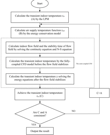
The flowchart of the semi-coupled CFD simulation of the transient indoor air temperature is described in Fig. 2. The three-dimensional transient indoor air temperature CFD model is built and solved in a commercial software Fluent. The supply air temperature of the fan coil is the boundary condition of the model. First, the initial time history of the supply air temperature is calculated by the LPM using equations (4) and (5). Second, the initial time history of the supply air temperature toutis input into a UDF (User Defined Function) as the initial boundary

(4)

Lu Zhang et al. / Energy Procedia 160 (2019) 420–427 423

[image:4.544.65.425.76.110.2]

operation state. This paper aims to simulate the transient room air temperature rising from the start to steady operation of the heat pump. The air is closed and circulated in the room. It is inhaled, heated, and then blown off by the fan coil. In the model, the velocity of the hot air blown off by the fan coil is assumed to be constant, but its temperature is changed with time. It is obvious that the velocity fields are largely unsynchronized with the temperature field changes, with velocity fields changing in seconds whereas temperature changing in minutes or even longer. Thus, the flow and the temperature fields are firstly solved by the fully coupled CFD simulation during the start-up period. Then the velocity fields are fixed and the discretized energy conservation equations are transformed into the fixed velocity fields to solve the transient air temperatures.

Fig. 1. The model of a HVAC bedroom

2.2.The three-dimensional transient indoor air temperature mathematical model

The three-dimensional transient room air temperature model can be described by mass conservation equation, momentum conservation equation, and energy equation.

Mass conservation equation (continuity equation):

0 u

v

w

x

y

z

ρ

τ

∂

₊

∂

₊

∂

₊

∂

₌

∂

(1)

Where ρ is density, kg/m3_;_u_,_v_,_w_{are components of velocity vector in}_x_,_y_,_z_{direction, respectively, m/s.}

N-S equation (momentum conservation equation):

2

x

y

z

u

_u

u

_v

u

_w

u

p

_g

_u

x

y

z

x

v

_u

v

_v

v

_w

v

p

_g

_v

x

y

z

y

w

_u

w

_v

w

_w

w

p

_g

_w

x

y

z

ρ

µ

τ

ρ

µ

τ

ρ

µ

τ



∂



∂

+

= −

+

+ ∇



_∂



_∂







∂

₊

∂

₊

∂

₊

∂



_{= −}

∂

₊

_{+ ∇}



_∂



_∂







∂

₊

∂

₊

∂

₊

∂



_{= −}

∂

₊

_{+ ∇}



_∂



_∂





(2)

Where ρis pressure, Pa; u is dynamic viscosity, Pa·s; g is acceleration of gravity, m/s2_;_{𝛻𝛻𝛻𝛻}2_{is Laplacian.}

Energy equation:

p

T

c

u

v

w

S

x

y

z

x

y

z

ρ

λ

τ



∂

₊

∂

₊

∂

₊

∂



₌

∂



∂



₊

∂



∂



₊

∂



∂



₊



_∂



_∂



_

_∂

_



_∂



_∂



_∂



_

_∂



_









(3)

Where S is internal heat source of the fluid, J; λ is thermal conductivity, W/(m·K).

For the HVAC bed-room, the indoor air flow is turbulent, and k-ε model is used to deal with the turbulent flow. The equations are discretized using the first order implicit scheme. In the semi-coupled CFD model, the transient continuity equation and N-S equation are solved firstly, and the stability time of the flow field is obtained. Secondly, the continuity equation, N-S equations, and energy equation are solved using the fully-coupled CFD method before the flow field is fixed. Thereafter, only the energy equation needs to be solved, and the transient indoor air temperature is obtained.

2.3.The boundary conditions and flowchart of the semi-coupled CFD model

The supply air temperature of the fan coil is used as a boundary condition in the model. The initial supply air temperature 𝑡𝑡𝑡𝑡𝑜𝑜𝑜𝑜𝑜𝑜𝑜𝑜𝑜𝑜𝑜𝑜is calculated by LPM. Heat transfer equation of the air in the fan coil is

(

)

2

in out

m p out in h

t

q c t

−

t

=

K A t



_

−

+



_



′



′

(4)

where is flowrate of the supply air from the fan coil, kg/s; cp is specific heat capacity of air, J/(kg·K); tout is the

supply air temperature, and it is changed with time; tin is the indoor air temperature and it is also the temperature of

the cold air inhaled by the fan coil, K; K’_A’_{is heat transfer performance of the fan coil, W/K, and it is acquired by}

parameters of the selected fan coil; th is the average wall temperature of the heat exchanger in the fan coil.

For the room air, the heat transfer is expressed according to energy conservation:

(

)

(

)

in

p

dt

m p out in chu o

mc

q c t

t

KA t

t

d

τ

=

−

(5)

Where m is mass of the indoor air, kg; τ is time, s; KA is the heat transfer performance of wall, W/K; to is ambient

temperature, K; tchu is initial indoor temperature before the heat pump starts, K.

The room air temperature history tin can be calculated through simultaneous equations (4) and (5), and then the

supply air temperature of the fan coil tout can be solved by equation (4). tout is a function of time, and it is the initial

boundary condition of the transient CFD model of the indoor air temperature.

The other boundary conditions of the transient indoor air temperature model are shown in Table. 1.

Table. 1. Boundary Condition

Boundary Interior wall / _floor Exterior wall Window Heat transfer

coefficient λ =0 W/(m2·K) λ =23 W/(m2·K) [9] λ =12 W/(m2·K) [9]

The flowchart of the semi-coupled CFD simulation of the transient indoor air temperature is described in Fig. 2. The three-dimensional transient indoor air temperature CFD model is built and solved in a commercial software Fluent. The supply air temperature of the fan coil is the boundary condition of the model. First, the initial time history of the supply air temperature is calculated by the LPM using equations (4) and (5). Second, the initial time history of the supply air temperature toutis input into a UDF (User Defined Function) as the initial boundary

(5)

424 Lu Zhang et al. / Energy Procedia 160 (2019) 420–427

is solved at the first iteration. Third, the time history of the supply air temperature tout is calculated using equation

[image:5.544.89.447.150.586.2]

(4), and the next iteration begins. If the indoor air temperature history calculated from one iteration matches with that of the next iteration within a defined tolerance, the simulation is considered converged. Otherwise, iterations will continue. For each iteration, the air velocity field and temperature field are solved using the fully-coupled CFD method at the first several time steps until the velocity field is stabilized, and then the flow field and the temperature field are segregated, and only the temperature field is solved based on the fixed velocity field.

Fig. 2. The flowchart of the simulation

3.Results and discussion

The transient indoor air temperature model is solved using the three different CFD models (the fully-coupled CFD model, the segregated CFD model, and the semi-coupled CFD model). The central point of the room is chosen as the monitoring point in the solving process. The temperature-time curves of the monitoring point at all iterations

The semi-coupled CFD

NO

YES Start

Calculate the transient indoor temperature tin (A) by the LPM

Calculate air supply temperature function tout (B) by the energy conservation model

Calculate indoor flow field and the stability time of flow field by solving the continuity equation and N-S equation

Calculate the transient indoor temperature by the fully-coupled CFD model before the flow field stabilizes

Calculate the transient indoor temperature y solving the energy equations after the flow field stabilizes

Achieve the transient indoor temperature tin (C)

Are C and A consistent?

Output the result

(6)

is solved at the first iteration. Third, the time history of the supply air temperature tout is calculated using equation

(4), and the next iteration begins. If the indoor air temperature history calculated from one iteration matches with that of the next iteration within a defined tolerance, the simulation is considered converged. Otherwise, iterations will continue. For each iteration, the air velocity field and temperature field are solved using the fully-coupled CFD method at the first several time steps until the velocity field is stabilized, and then the flow field and the temperature field are segregated, and only the temperature field is solved based on the fixed velocity field.

Fig. 2. The flowchart of the simulation

3.Results and discussion

The transient indoor air temperature model is solved using the three different CFD models (the fully-coupled CFD model, the segregated CFD model, and the semi-coupled CFD model). The central point of the room is chosen as the monitoring point in the solving process. The temperature-time curves of the monitoring point at all iterations

The semi-coupled CFD

NO

YES Start

Calculate the transient indoor temperature tin (A) by the LPM

Calculate air supply temperature function tout (B) by the energy conservation model

Calculate indoor flow field and the stability time of flow field by solving the continuity equation and N-S equation

Calculate the transient indoor temperature by the fully-coupled CFD model before the flow field stabilizes

Calculate the transient indoor temperature y solving the energy equations after the flow field stabilizes

Achieve the transient indoor temperature tin (C)

Are C and A consistent?

Output the result

C=A

are shown in Fig.3. The curve tin(0) is the temperature-time curve calculated using LPM described by equations (4)

and (5). Then the supply air temperature tout(1) is calculated from tin(0), and is applied as the initial boundary

condition of the transient room air temperature model for the first iteration. The curve tin (1) is the result of the first

iteration. A new supply air temperature tout(2) is calculated according to the curve tin (1) and it is the boundary

condition of the second iteration. And so on, if the temperature-time curve of tin (n) calculated from the nth iteration

matches with that of the (n+1)th_{iteration within a defined tolerance, the results are considered converge. The}

calculation results of the three CFD models are shown in Fig. 3. Fig. 3 (a), (b), and (c) represent the results of the coupled CFD model, the segregated CFD model and the semi-coupled CFD model respectively. For the fully-coupled CFD model, the velocity and the temperature fields are fully-fully-coupled at each time step for each an iteration. It is expected to simulate the real temperature rising process best, and have the most accurate simulation results in the three CFD models. It was found that the simulations were converged after 3 iterations for each CFD model. The converged results of the three CFD models are shown in Fig. 4. It revealed that temperature-time curve of tin of the

semi-coupled CFD model has a good agreement with that obtained from the fully-coupled CFD model.But for the segregated CFD model, the results had great differences from that of the fully-coupled CFD model at the early stage of temperature rising, and then they matched well at the late stage.

0 10 20 30 40 50 60 70 80 90 100

0 2 4 6 8 10 12 14 16 18 20 22 24 26

Tin

(

oC)

Flow time (s) tin(1)

tin(2)

tin(3)

tin(4)

a

0 10 20 30 40 50 60 70 80 90 100

0 2 4 6 8 10 12 14 16 18 20 22 24 26

Tin

(

oC)

time (s) tin(1)

tin(2) tin(3) tin(4) b

0 10 20 30 40 50 60 70 80 90 100

0 2 4 6 8 10 12 14 16 18 20 22 24 26

Tin

(

oC)

time (s) tin(1)

[image:6.544.82.462.276.554.2]

tin(2) tin(3) tin(4) c

(7)

426 Lu Zhang / Energy Procedia 00 (2018) 000–000 Lu Zhang et al. / Energy Procedia 160 (2019) 420–427 7

0 10 20 30 40 50 60 70 80 90 100

0 2 4 6 8 10 12 14 16 18 20 22 24 26

Tin

(

oC)

[image:7.544.187.359.78.202.2]

time (s) the fully-coupled CFD model the segregated CFD model the semi-coupled CFD model

Fig. 4. The final transient indoor temperature iteration curves of three different CFD models

The indoor air temperature is expected to be kept at 20 °C in winter, so the heat pump steps into the stable operation state when the indoor temperature reaches 20 °C. The computational time of three different CFD models is defined as the time when tin reaches 20 °C, and the results are summarized in Table. 2. It was found that the

fully-coupled CFD model had the longest computational time of 6 hours, and the segregated CFD model and the semi-coupled CFD model have much shorter computation time of 2 hours and 3 hours respectively.

Table. 2. Computation time and results of three different CFD models

Three different CFD models The computation time the stability time of flow field Results time for the indoor air temperature reaches to 20℃

the fully-coupled CFD model about 6 hours / 82 s

the segregated CFD model about 2 hours / 77 s

the semi-coupled CFD model about 3 hours 13 s 75 s

4.Conclusions

This paper proposed a semi-coupled CFD model combining advantages of the fully-coupled CFD model and the segregated CFD model to simulate transient air temperature rising of a HVAC room from a start temperature to a pre-set room temperature. The efficiency of the proposed model was compared with the fully-coupled CFD model and the segregated CFD model. The results showed that all three simulation models could converge within three iterations. The comparison results showed that the proposed model had the similar simulation accuracy as the fully-coupled CFD model. However, the computational time was only half of the fully-fully-coupled model. Although the segregated CFD model showed the shortest computational time, the computational accuracy was far lower than those from the fully-coupled and the proposed model at the beginning stage. These analyses demonstrated that the proposed model can be reliably used to investigate the indoor air temperature with a sound simulation accuracy and reasonable computational time.

Acknowledgements

This work is supported by the National Science Foundation of China [No.51676150]. The authors are grateful for the support by the project named of "Heating load analyses of typical suburban residential buildings of Chinese different regions (5202011600U4)" in China State Grid Corp.

References

(8)

0 10 20 30 40 50 60 70 80 90 100

0 2 4 6 8 10 12 14 16 18 20 22 24 26

Tin

(

oC)

time (s) the fully-coupled CFD model the segregated CFD model the semi-coupled CFD model

Fig. 4. The final transient indoor temperature iteration curves of three different CFD models

The indoor air temperature is expected to be kept at 20 °C in winter, so the heat pump steps into the stable operation state when the indoor temperature reaches 20 °C. The computational time of three different CFD models is defined as the time when tin reaches 20 °C, and the results are summarized in Table. 2. It was found that the

fully-coupled CFD model had the longest computational time of 6 hours, and the segregated CFD model and the semi-coupled CFD model have much shorter computation time of 2 hours and 3 hours respectively.

Table. 2. Computation time and results of three different CFD models

Three different CFD models The computation time the stability time of flow field Results time for the indoor air temperature reaches to 20℃

the fully-coupled CFD model about 6 hours / 82 s

the segregated CFD model about 2 hours / 77 s

the semi-coupled CFD model about 3 hours 13 s 75 s

4.Conclusions

This paper proposed a semi-coupled CFD model combining advantages of the fully-coupled CFD model and the segregated CFD model to simulate transient air temperature rising of a HVAC room from a start temperature to a pre-set room temperature. The efficiency of the proposed model was compared with the fully-coupled CFD model and the segregated CFD model. The results showed that all three simulation models could converge within three iterations. The comparison results showed that the proposed model had the similar simulation accuracy as the fully-coupled CFD model. However, the computational time was only half of the fully-fully-coupled model. Although the segregated CFD model showed the shortest computational time, the computational accuracy was far lower than those from the fully-coupled and the proposed model at the beginning stage. These analyses demonstrated that the proposed model can be reliably used to investigate the indoor air temperature with a sound simulation accuracy and reasonable computational time.

Acknowledgements

This work is supported by the National Science Foundation of China [No.51676150]. The authors are grateful for the support by the project named of "Heating load analyses of typical suburban residential buildings of Chinese different regions (5202011600U4)" in China State Grid Corp.

References

[1] Bozkır O, Canbazoğlu S. Unsteady thermal performance analysis of a room with serial and parallel duct radiant floor heating system using hot airflow[J]. Energy & Buildings, 2004, 36(6):579-586.

[2] Romano F, Colombo L P M, Gaudenzi M, et al. Passive control of microclimate in museum display cases: A lumped parameter model and experimental tests [J]. Journal of Cultural Heritage, 2015, 16(4):413-418.

[3] Popovici C G. HVAC System Functionality Simulation Using ANSYS-Fluent [J]. Energy Procedia, 2017, 112:360-365.

[4] Fang P, Liu T, Liu K, et al. A Simulation Model to Calculate Temperature Distribution of an Air-Conditioned Room[C]// International Conference on Intelligent Human-Machine Systems and Cybernetics. IEEE, 2016.

[5] HaidongWang, Zhiqiang(John)Zhai. Application of coarse-grid computational fluid dynamics on indoor environment modeling: Optimizing the trade-off between grid resolution and simulation accuracy [J]. Hvac & R Research, 2012, 18(5):915-933.

[6] Zuo W, Chen Q. Real‐time or faster‐than‐real‐time simulation of airflow in buildings [J]. Indoor Air, 2009, 19(1):33-44.

[7] Wang Q, Pan Y, Zhu M, et al. A state-space method for real-time transient simulation of indoor airflow [J].Building & Environment, 2017, 126.

[8] Tian W, Sevilla T A, Li D, et al. Fast and self-learning indoor airflow simulation based on in situ adaptive tabulation[J]. Journal of Building Performance Simulation, 2018.