The first planetary microlensing event with two microlensed source stars

The First Planetary Microlensing Event with Two Microlensed Source Stars

D. P. Bennett1,2,40,41 , A. Udalski3,42, C. Han4,43 , I. A. Bond5,40, J.-P. Beaulieu6,41 , J. Skowron3,42 , B. S. Gaudi7,43 , N. Koshimoto1,8,40 , F. Abe9, Y. Asakura9, R. K. Barry1, A. Bhattacharya1,2, M. Donachie10, P. Evans10, A. Fukui11 , Y. Hirao8,

Y. Itow9 , M. C. A. Li10, C. H. Ling5, K. Masuda9, Y. Matsubara9, Y. Muraki9, M. Nagakane8, K. Ohnishi12, H. Oyokawa9, C. Ranc1, N. J. Rattenbury10 , M. M. Rosenthal13, To. Saito14, A. Sharan10, D. J. Sullivan15, T. Sumi8, D. Suzuki16 ,

P. J. Tristram17, A. Yonehara9 (The MOA Collaboration),

M. K. Szymański3, R. Poleski3,7, I. Soszyński3, K. Ulaczyk3,Ł. Wyrzykowski3 (The OGLE Collaboration),

D. DePoy18, A. Gould7,19,20, R. W. Pogge7 , J. C. Yee21 (TheμFUN Collaboration),

and

M. D. Albrow22 , E. Bachelet23 , V. Batista6 , R. Bowens-Rubin24, S. Brillant25, J. A. R. Caldwell26 , A. Cole27, C. Coutures6, S. Dieters27, D. Dominis Prester28, J. Donatowicz29, P. Fouqué30,31, K. Horne32 , M. Hundertmark32,33 , N. Kains34 , S. R. Kane35 , J.-B. Marquette6, J. Menzies36, K. R. Pollard22, C. Ranc1, K. C. Sahu34 , J. Wambsganss37 ,

A. Williams38,39, and M. Zub37 (The PLANET Collaboration)

1

Code 667, NASA Goddard Space Flight Center, Greenbelt, MD 20771, USA;[email protected] 2

Department of Astronomy, University of Maryland, College Park, MD 20742, USA

3

Warsaw University Observatory, Al.Ujazdowskie4, 00-478Warszawa, Poland

4

Department of Physics, Chungbuk National University, Cheongju 361-763, Republic of Korea

5

Institute of Natural and Mathematical Sciences, Massey University, Auckland 0745, New Zealand

6_{Institut d’Astrophysique de Paris, 98 bis bd Arago, F-75014 Paris, France} 7

Department of Astronomy, Ohio State University, 140 West 18th Avenue, Columbus, OH 43210, USA

8

Department of Earth and Space Science, Graduate School of Science, Osaka University, Toyonaka, Osaka 560-0043, Japan

9

Institute for Space-Earth Environmental Research, Nagoya University, Nagoya 464-8601, Japan

10

Department of Physics, University of Auckland, Private Bag 92019, Auckland, New Zealand

11

Okayama Astrophysical Observatory, National Astronomical Observatory of Japan, 3037-5 Honjo, Kamogata, Asakuchi, Okayama 719-0232, Japan

12

Nagano National College of Technology, Nagano 381-8550, Japan

13

Department of Astronomy and Astrophysics, University of California, Santa Cruz, CA 95064, USA

14

Tokyo Metropolitan College of Aeronautics, Tokyo 116-8523, Japan

15_{School of Chemical and Physical Sciences, Victoria University, Wellington, New Zealand} 16

Institute of Space and Astronautical Science, Japan Aerospace Exploration Agency, Kanagawa 252-5210, Japan

17

University of Canterbury Mt. John Observatory, P.O. Box 56, Lake Tekapo 8770, New Zealand

18

Department of Physics, Texas A&M University, 4242 TAMU, College Station, TX 77843-4242, USA

19

Max-Planck-Institute for Astronomy, Königstuhl 17, D-69117 Heidelberg, Germany

20

Korea Astronomy and Space Science Institute, Daejon 34055, Republic of Korea

21

Harvard-Smithsonian Center for Astrophysics, 60 Garden Street, Cambridge, MA 02138, USA

22

University of Canterbury, Department of Physics and Astronomy, Private Bag 4800, 8020 Christchurch, New Zealand

23

Las Cumbres Observatory Global Telescope Network, 6740 Cortona Drive, suite 102, Goleta, CA 93117, USA

24

Department of Earth, Atmospheric and Planetary Sciences, Massachusetts Institute of Technology, 77 Massachusetts Ave., Cambridge, MA 02139, USA

25

ESO Vitacura, Alonso de Crdova 3107. Vitacura, Casilla 19001, Santiago 19, Chile

26_{McDonald Observatory, 82 Mt Locke Road, TX 79734, USA} 27

School of Math and Physics, University of Tasmania, Private Bag 37, GPO Hobart, 7001 Tasmania, Australia

28

Department of Physics, University of Rijeka, Radmile Matej vcić2, 51000 Rijeka, Croatia

29

Technical University of Vienna, Department of Computing, Wiedner Hauptstrasse 10, A-1040 Wien, Austria

30

CFHT Corporation, 65-1238 Mamalahoa Hwy, Kamuela, Hawaii 96743, USA

31

IRAP, CNRS—Université de Toulouse, 14 av. E. Belin, F-31400 Toulouse, France

32

SUPA, School of Physics & Astronomy, University of St Andrews, North Haugh, St Andrews KY16 9SS, UK

33

Niels Bohr Institutet, Københavns Universitet, Juliane Maries Vej 30, DK-2100 København Ø, Denmark

34

Space Telescope Science Institute, 3700 San Martin Drive, Baltimore, MD 21218, USA

35_{Department of Earth Sciences, University of California, Riverside, CA 92521, USA} 36

South African Astronomical Observatory, PO Box 9, Observatory 7935, South Africa

37

Astronomisches Rechen-Institut, Zentrum für Astronomie der Universität Heidelberg(ZAH), Mönchhofstraße 12-14, D-69120 Heidelberg, Germany

38

Perth Observatory, Walnut Road, Bickley, Perth 6076, Australia

39

International Centre for Radio Astronomy Research, Curtin University, Bentley, WA 6102, Australia Received 2017 July 27; revised 2018 February 2; accepted 2018 February 6; published 2018 March 7

© 2018. The American Astronomical Society. All rights reserved.

40

MOA Collaboration.

41

PLANET Collaboration.

42

OGLE Collaboration.

43

Abstract

We present the analysis of the microlensing event MOA-2010-BLG-117, and show that the light curve can only be explained by the gravitational lensing of a binary source star system by a star with a Jupiter-mass ratio planet. It was necessary to modify standard microlensing modeling methods tofind the correct light curve solution for this binary source, binary-lens event. We are able to measure a strong microlensing parallax signal, which yields the masses of the host star, M_*=0.58±0.11 Me, and planet, mp=0.54±0.10MJup, at a projected star–planet

separation of a⊥=2.42±0.26 au, corresponding to a semimajor axis of a =2.9+_-1.6_0.6 au. Thus, the system resembles a half-scale model of the Sun–Jupiter system with a half-Jupiter0mass planet orbiting a half-solar-mass star at very roughly half of Jupiter’s orbital distance from the Sun. The source stars are slightly evolved, and by requiring them to lie on the same isochrone, we can constrain the source to lie in the near side of the bulge at a distance ofDS=6.9±0.7 kpc, which implies a distance to the planetary lens system ofDL=3.5±0.4 kpc. The

ability to model unusual planetary microlensing events, like this one, will be necessary to extract precise statistical information from the planned large exoplanet microlensing surveys, such as theWFIRSTmicrolensing survey.

Key words:gravitational lensing: micro– planetary systems

1. Introduction

Gravitational microlensing has a unique niche among planet discovery methods(Bennett2008; Gaudi2012)because of its sensitivity to planets with masses extending to below an Earth mass (Bennett & Rhie 1996) orbiting beyond the snow line (Mao & Paczyński1991; Gould & Loeb1992), where planet formation is thought to be the most efficient, according to the leading core accretion theory of planet formation (Lissauer

1993; Pollack et al.1996). While radial velocity and planetary transit surveys (Ida & Lin 2005; Kennedy et al. 2006; Lecar et al. 2006; Kennedy & Kenyon 2008; Thommes et al. 2008; Wright & Gaudi 2013; Twicken et al. 2016) have found hundreds and thousands of planets, respectively, these methods have much higher sensitivity to planets that orbit very close to their host stars. Their sensitivity to planets like those in our own solar system is quite limited. Our knowledge of these wide-orbit planets extending down to low masses depends on the results of microlensing surveys(Gould et al.2010b; Cassan et al.2012; Suzuki et al.2016). This is the main reason for the selection of the space-based exoplanet microlensing survey (Bennett & Rhie 2002) to be a part of the WFIRST mission (Spergel et al. 2015), which was the top-rated large space mission in the 2010 New Worlds, New Horizons decadal survey.

Like the Kepler transit survey (Borucki et al. 2011), the

WFIRST exoplanet microlensing survey will primarily be a statistical survey with thousands of expected exoplanet discoveries. However, a large number of planet discoveries does not automatically translate into good statistics if a large fraction of the planet candidates do not allow precise interpretations (Burke et al. 2015; Mullally et al. 2016). Fortunately, the microlensing method predicts a relatively small number of low signal-to-noise planet candidates (Gould et al. 2004) compared to the transit method. Nevertheless, microlensing does have the potential problem of microlensing events that defy interpretation, and these could also add to the statistical uncertainty in the properties of the exoplanet population that can be studied by microlensing.

In the past two years, the analysis of several complicated microlensing events potentially involving planets has been completed. The lens system for OGLE-2007-BLG-349 was revealed to be a circumbinary planet, rather than a two-planet system with a single host star (Bennett et al. 2016). This removed a significant uncertainty from the Gould et al. (2010b), Cassan et al. (2012), and Suzuki et al. (2016)

statistical analyses, which included this event. (If the two-planet model for OGLE-2007-BLG-349 had been correct, the second planet would have been the lowest mass ratio planet discovered by microlensing.) Another complicated event was OGLE-2013-BLG-0723, which was originally claimed to be a planet in a binary star system that was unusually close to the Sun for a microlensing event(Udalski et al.2015a). This small distance to the lens system was due to a large microlensing parallax signal. However, a more careful analysis of the data (Han et al. 2016) indicated that the light curve was better explained by a binary star system without a planet and a much smaller microlensing parallax signal. Most recently, Han et al. (2017)analyzed a planet in a binary star system and found a somewhat ambiguous result, with solutions consisting of a planet and stellar (or brown dwarf) hosts with mass ratios ranging from 0.95 to 0.03.

In this paper, we present the analysis of the microlensing event MOA-2010-BLG-117, an event that has eluded precise interpretation for several years after it was observed and identified as a planetary microlensing event. It has a strong planetary signal, so it must be included in the statistical analysis of MOA data (Suzuki et al. 2016). In fact, the basic character of the light curve was obvious by inspection to many of the authors of this paper. There was a clear planetary signal due to the crossing of two minor image caustics, but detailed models did not provide a good fit. The region between these two minor image caustics is an area of strong demagnification because the minor image is largely destroyed in this region, but the magnification between MOA-2010-BLG-117 was simply too large. It could only befit with the addition of a fourth body to increase the magnification between the minor image caustics. This fourth body could be a second source star that would not pass between the minor image caustics and would therefore not suffer the demagnification experienced by the first source. Or the fourth body could be a third lens that could provide additional magnification between the minor image caustics. We found that the only viable triple-lens systems were ones the with two stars orbited by one planet, and that two-planet models could not match the observed light curve. The early modeling could not decide between the binary source and circumbinary planet possibilities.

This paper is organized as follows. In Section2, we describe the light curve data, photometry, and real-time modeling that influenced some of the data collection strategy. In Section3, we describe the systematic light curve modeling of the final data set, which shows that the binary source model must be

correct. We also show that we can constrain the distance to the source by requiring that the two source stars have magnitudes and colors that lie on the same isochrone. We describe the photometric calibration and the determination of the primary source star radius in Section 4, and then we derive the lens system properties in Section5. In Section6, we consider high angular resolution adaptive optics (AO) observations of the MOA-2010-BLG-117 target, and we present a proper motion measurement of the MOA-2010-BLG-117 target that indicates that the source star system lies in the Galactic bulge. Our conclusions are presented in Section 7.

2. Light Curve Data, Photometry and Real Time Modeling

The microlensing event MOA-2010-BLG-117, at R.A.= 18:07:49.67, decl.=−25:20:40.7, and Galactic coordinates (l,b)=(5.5875,−2.4680), was identified and announced as a microlensing candidate by the Microlensing Observations in Astrophysics (MOA) Collaboration Alert system (Bond et al. 2001) on 2010 April 7. The MOA team subsequently identified the light curve as anomalous at UT 10:19 am, 2010 August 2, and this announcement triggered follow-up observa-tions by the Probing Lensing Anomalies NETwork(PLANET) and the MICROlensing Follow-up Network (μFUN). The PLANET group observed this event using the 1.0 m telescope at the South African Astronomical Observatory (SAAO), and theμFUN group used the 1.3 SMARTS telescope at the Cerro Tololo Interamerican Observatory (CTIO). The Optical Grav-itational Lensing Experiment (OGLE) Collaboration had just updated to their wide field of view OGLE-4 system(Udalski et al.2015b), and their Early Warning System(EWS)was not yet in operation with the new camera(Udalski et al.1994). So, the OGLE photometry was not produced automatically by the EWS system, but once it became clear that this event had a likely planetary signal, OGLE began to reduce and circulate their data.

After some systematic trends with airmass were removed from the MOA data and the OGLE data was released, it became clear by inspection that the light curve of this event resembled the case of a source that crossed the region of the triangular minor image caustics, hitting both caustics. This configuration is somewhat similar to that of OGLE-2007-BLG-368 (Sumi et al. 2010) and MOA-2009-BLG-266 (Muraki et al. 2011), except that the source for OGLE-2007-BLG-368 only crossed one of the minor image caustics and the source for MOA-2009-BLG-266 was almost as large as the minor image caustics. However, attempts to model this event did not yield good fits with this geometry.

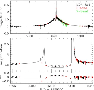
The problem with this minor image caustic-crossing model is that the magnification deficit between the two caustic(or cusp) crossings at t=5402 and 5411 is too small. (Note that t≡

HJD−2450000). This is evident in Figure1, which shows the best-fit binary-lens light curve for MOA-2010-BLG-2010. This light curve has the obvious problem that the magnification between the two caustic/cusp features is higher than the model can accommodate. In fact, the problem is more severe than this

figure indicates. In order to minimize this discrepancy between the model and the data, the event is driven to have a very bright source, so that the minor image will be kept at relatively low magnification, which reduces the magnification deficit between the two caustic/cusp features. However, in this case, the source brightness is driven to be1.5´brighter than the apparent source star in the OGLE images. This means that negative blending is

required, since a negative “blend flux” must be added to the source flux to achieve the relatively faint “star” seen in the unmagnified images. Negative blending is quite possible at low levels due to the variations in the apparent“sky”background due to unresolved stars, but in this case, the level of negative blending is too large for such a physical explanation. So, it implies that this model is likely to be incorrect.

Because of these difficulties with the minor image perturba-tion model and unrelated difficulties with the real-time photometry, early attempts at modeling this event predicted that the relatively bright, well-observed feature att≈5411 was the interior of a caustic entrance, where the caustic crossing itself was not observed. But, a subsequent caustic exit never occurred. This made it clear that some version of a planetary minor caustic-crossing event was correct, but that an additional lens or source was needed to explain the higher-than-expected brightness between the two caustic/cusp crossings. This possibility was recognized relatively early after the discovery of the light curve anomaly, so we obtained more frequent CTIO

V-band observations than usual in the hopes that they might help reveal a color difference between the two sources of a binary source model.

It was necessary to wait until mid-2011 before the magnification was back at baseline because of the long duration of this microlensing event. After that, the OGLE Collaboration provided optimal centroid photometry using the OGLE difference imaging pipeline(Udalski2003). Photometry of the MOA data was performed with the MOA pipeline(Bond et al.2001), which also employs the difference imaging method (Tomaney & Crotts 1996). The PLANET collaboration’s SAAO data were reduced with a version of the Pysis difference imaging code (Albrow et al. 2009), and the CTIO data were reduced with DoPHOT(Schechter et al. 1993). Thefinal data set consists of 4966 MOA observations in the custom MOA-Red passband(roughly equivalent to the sum of CousinsR+I), 398 and 48 OGLE observations in the I and V bands, respectively, 150 I-band and 88 V-band observations from the SMARTS telescope in CTIO, 119I-band observations from SAAO, and 10 K-band observations from the VVV survey (Minniti et al. 2010) using the VISTA telescope at Paranal, which happened to be doing a low-cadence survey of the Galactic bulge in 2010.

3. Light Curve Models

Our light curve modeling was done using the image-centered ray-shooting method (Bennett & Rhie 1996; Bennett 2010), supplemented with the hexadecapole approximation (Gould

2008; Pejcha & Heyrovský2009)that is employed as a test for accuracy. For triple-lens modeling, we used the code developed for OGLE-2006-BLG-109 (Bennett et al. 2010) and OGLE-2007-BLG-349(Bennett et al. 2016). Triple-lens models have some parameters in common with single- and binary-lens models. These are the Einstein radius crossing time,tE, and the

time,t0, and distance,u0, of closest approach between the lens’ center of mass and the source star. For a binary lens, there is also the mass ratio of the secondary to the primary lens,q, the angle between the lens axis and the source trajectory,θ, and the separation between the lens masses,s.

The length parameters, u0 and s, are normalized by the Einstein radius of this total system mass, RE =

GM c D x x

4 2 S 1

-( ) ( ), where x=DL/DS, and DL and DS

the gravitational constant and speed of light, as usual.) For triple-lens models, there are additional separation, mass ratio, and angle to describe the position and mass ratio of the third lens, but we will not explore these models in detail in this paper.

For every passband, there are two parameters to describe the unlensed source brightness and the combined brightness of any unlensed “blend” stars that are superimposed on the source. Such“blend”stars are quite common because microlensing is only seen if the lens–source alignment isθ_E∼1 mas, while stars are unresolved in ground-based images if their separation is 1″. However, with ground-based seeing, the background contains many unresolved stars, and this makes the background uneven. As a result, it is possible to have realistic cases of

“negative blending”if the“negative”brightness of the blend is consistent with the fluctuations in the unresolved stellar background. Artificial negative blending can occur with difference imaging photometry, which does not attempt to identify a source star in the reference image, but this is just an artifact of the photometry method. In any case, these source and blend fluxes are treated differently from the other parameters because the observed brightness has a linear dependence on them, so for each set of nonlinear parameters, we canfind the source and blend fluxes that minimize the χ2 exactly, using standard linear algebra methods (Rhie et al.1999).

For the binary source models for MOA-2010-BLG-117, we add a second source to the binary-lens model, allowing for a different brightness and color for the second source. The second source has its ownt0andu0values, which we denote as

t0 2s and u0 2s . If the two source stars have exactly the same velocity, then the tE and θ values for the two sources would

also be the same, but due to orbital motion, thetEandθvalues

are slightly different. However, the orbital motion of the source stars is much smaller than the orbital motion of the source star system in the Galaxy, so we use parameters to describe the difference in thetEand θ values. The parameters we use are

dtEs2=tEs2-tEs1 and dθs2=θs2−θs1, where tE=tEs1 and

θ=θs1.

Our initial attempts to model this event favored the circumbinary models, and the model shown in Figure 2 was the best fit. However, there are several problems with this model. First, although the data are sparse, the model does not provide a goodfit to thefirst cusp approach att=5402–5403. However, there is a more serious problem with this model that is demonstrated by Figure 3, which shows how the orbital motion of the binary host stars affects the caustic configuration. The central caustic rotates quite rapidly, such that the angle between the direction of the right-pointing cusp and the source position remains nearly constant throughout the interval between the cusp crossings. This is apparently necessary to avoid having a local light curve peak in the middle of the long minimum at 5403.5<t<5410 at a location where the cusp would be pointing directly at the source. With the rapid orbital motion implied by this model, the source can remain at the same angle with respect to the cusp direction throughout the passage of this light curve minimum.

The rapid orbital motion presents a problem, however. The probability of lensing by two stars that are not bound to each other is quite small (∼10−12), so we can assume that the two lens stars are bound. If so, then their relative velocity cannot be above the escape velocity of the system. As a result, the high relative velocity implies that the lens must be close to either the

Figure 1.Best binary-lens model for the MOA-2010-BLG-117 light curve. MOA-Red band data are shown in black.I-band data from OGLE, CTIO, and SAAO are shown in red, light red, and dark red, respectively, while the OGLE and CTIOV-band data are shown in green and light green.

lens or the observer, because both of these possibilities allow higher lens orbital velocities when measured in units of Einstein radii per unit time. With the angular source radius,q_*, derived below in Section4, we can derive the angular Einstein radius, θ_E=θ_* tE/t*, and this yields the following relation

(Bennett2008; Gaudi2012)

M c

G

D D

D D M

x x

D

4 0.9823

1 mas 1 8 kpc , 1

L E

S L

S L

E S

2 2

2

q

q =

- =

´

-

⎜ ⎟ ⎜ ⎟

⎛

⎝ ⎞⎠ ⎛⎝ ⎞⎠ ⎛ ⎝

⎜ ⎞

⎠

⎟ ( )

wherex=DL DSandθE∼0.8 mas for this event. This allows

us to determine the lens system mass and convert the measured transverse separation and velocity to physical units at every possible distance for the lens. This exercise tells us that the two stars would be unbound for 0.93 kpc<DL<7.5 kpc and

0.05Me<ML<26Me. However, the microlensing parallax

parameters for this model imply a lens system mass of

ML=0.218Me. We can conclude that the lens orbital velocity

parameters are too large for a physically reasonable model, and so the binary source model is favored.

Although the best circumbinary model implied unphysical parameters, in our initial modeling, the best circumbinary model had a better χ2than the best binary source models that we found, by Δχ2>130. However, the best binary source models from ourfirst round offitting had an unphysical feature as well. As with the models with a single source, we had been considering the source brightnesses in each passband as independent parameters. But, this allowed the models to move

into unphysical regions of the parameter space, in which the

flux ratio between the two sources was very different for passbands that were nearly identical, like the OGLE, CTIO, and SAAOIbands. In order to avoid these unphysical models, we have modified our modeling code tofix the sourceflux ratio to be the same for each of theI-band data sets and each of the

V-band data sets. Theflux ratio of source 2 to source 1 is given by the parameters f_{s V2} and f_{s I2} in the V and I bands, respectively. Source 1 is defined to be the source that crosses the planetary caustics. For the MOA-Red band, we do not use a independentflux ratio parameter. Instead, we derive the MOA-Red band flux ratio parameter from the I- and V-band parameters, f_{s Rm2} =f_{s I}0.837₂ f_{s V}0.163₂ . This follows from the color transformation that we have derived from the bright stars in this

field(Gould et al.2010a; Bennett et al.2012),

Rmoa -IO4=0.1630(VO4-IO4)+const, ( )2

where VO4and IO4 refer to the OGLE-IV V-band and I-band magnitudes that have been used for the OGLE light curve data. Note that these restrictions are more restrictive than those used for some previous non-planetary binary source events that only constrained data sets using the same passband with the same

flux ratio(Hwang et al.2013; Jung et al. 2017).

With these limitations on the source brightness ratios, we found that the binary source models quickly converged to a solution that was better than the previous best binary source model by _Dc2_~200_{. It was also better than the best}

circumbinary model byΔχ2=68.9, even though we allowed some of the parameters of the best circumbinary model to take unphysical values.

The best-fit light curve model is shown in Figure4, with the parameters listed in the third column of Table 1.(The best-fit solution withu0<0 is listed in the fourth column.)Because the sources have different colors, the light curves in the different passbands are different. The green, red, and black curves represent the model light curves in the V, I, and Rmoa

passbands, respectively. The data are plotted with a similar color scheme. We use green and light green for the OGLE and CTIOV-band data, black for theRmoadata, and dark red, red, and light red for the SAAO, OGLE, and μFUN I-band data, respectively. The caustic configuration for the best-fit model is shown in Figure 5. We define the source that crosses the planetary caustic to be source number 1 and the other to be source 2. Although both sources have similar∣ ∣u0 ~0.3and

u0 2s ~0.3

∣ ∣ values, we know that only one source comes close to the planetary caustics since we see no evidence of a second encounter of the planetary caustics. This implies that the two sources must pass on different sides of the planetary host star so that the signs of u0andu0 2s must be different.

The model parameters for the best-fit models with u0>0 and u0<0 are given in Table 1. Table 2 gives the Markov Chain Monte Carlo (MCMC) averages for the model parameters. This table also includes some derived parameters of physical interest: the angular Einstein radius, qE, the microlensing parallax amplitude, pE = pE E2, +pE N2, , and

the lens–source relative proper motion, m_rel,G, in an inertial geocentric frame that moves with the Earth at time

tfix=5411 days. The source–lens relative velocities for the two sources should be approximately equal because the orbital

velocity of two stars separated by approximately an Einstein radius in the Galactic bulge is typically about an order of magnitude smaller than the orbital velocity of stars in the inner Galaxy. So, we expect the lens–source relative velocity vectors for the two sources to differ by no more than∼10%. However, a ∼10% difference between the tE and θ values for the two

sources will have a significant effect on the light curve shape, so we must include parameters to describe tE and θ for the

second source. We chose the parameters dtEs2ºtEs2-tEs1,

wheretEs1ºtE,and tEs2are thetEvalues for the two sources.

The different source trajectory angles are described by

dqs2ºqs2-qs1, whereqs1ºqandqs2 are the angles between

the source trajectories and the lens axis. We also allow for orbital acceleration of the two source stars. We assume a circular orbit for these stars with an orbital period ofTSorband

projected velocities at time tfix=5411 days implied by the

dtEs2 and dqs2 values. These are circular orbits in three

dimensions following the parameterization of Bennett et al. (2010).

The orbital velocities in the lens system are also important, but since the planetary features in the light curve are detectable for only ∼10 days, we do not need to include the orbital acceleration of the source. We describe the lens orbital velocities with a rotation of the lens system with angular frequencyωand a velocity ofs˙in the separation direction.

This event has a significant orbital microlensing parallax signal (Gould 1992; Alcock et al. 1995), with a χ2 improvement ofΔχ2=43.93 with nearly equal contributions from the MOA and OGLE data sets. The microlensing parallax is defined by a two-dimensional vector,pE,with the north and

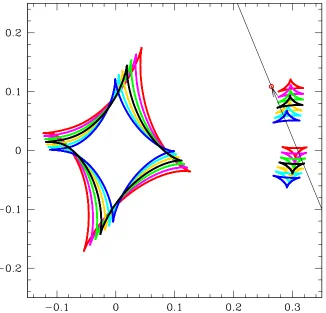
Figure 3.Caustic configuration, shown at an interval of two days for the best circumbinary-lens model for the MOA-2010-BLG-117 light curve. The caustics are shown att=5401, 5403, 5405, 5407, 5409, 5411, and 5413 in red, magenta, green, black, gold, cyan, and blue, respectively. The source trajectory is given by the black line with the red circle indicating the source size.

east components of π_E,N and πE,E in a geocentric coordinate

system moving with the velocity of the Earth measured at time

tfix=5411 days. The parameter tfix is also the reference time for the source and lens positions.

We should note that there are upper limits on the relative velocities between the two sources and between the lens star

and planet since they must(almost certainly)be gravitationally bound systems. We assume that the source stars each have a solar mass and compare the two-dimensional kinetic energy to the maximum binding energy of the source stars (using their separation on the plane of the sky). Then, following Muraki et al.(2011), we apply a constraint on thedtEs2anddqs2values.

For the lens system, we know the lens mass from the microlensing parallax parameters and the angular Einstein radius, θ_E(Gould 1992; Bennett 2008; Gaudi 2012), and we use this to apply the same constraint. In both cases, the orbital semimajor axis is proportional toθ_E.

These lens and source orbital motion constraints are sensitive to the source radius crossing time throughqE =tEq_{* *}t , but the

light curve constraint on t_* is relatively weak because the caustic crossings are only partially covered. The initialfits to this event with no microlensing parallax, no lens orbital motion, anddtEs2º0 anddqs2º0had a large variation in t*

values ranging from 0.24 to 0.40 days. When we allowed the

dtEs2anddqs2values to vary, subject only to the constraint on

the maximum orbital motion of the source stars, we found that large values of these parameters were preferred. However, the semimajor axis of the orbit of the source stars is proportional to θE=tE θ*/t*. Thus, a larger t* implies a smaller θE and

therefore a smaller semimajor axis. The smaller semimajor axis implies a higher gravitational binding energy, which allows larger lens star velocities, implying larger values fordtEs2and dqs2. Since the data apparently prefer larger values fordtEs2and dqs2, the constraint ont*becomes tighter when we include

non-zero values of dtEs2 and dqs2, and apply the orbital motion

constraint. This can be seen from Figure 6. Values of

t_*<0.26 days are excluded, and the 2σ lower limit on t_* is

Figure 4.Best binary source model for the MOA-2010-BLG-117 light curve. TheI-band light curves are plotted in different shades of red, with SAAO as dark red, OGLE as red, and CTIO as light red. The OGLE and CTIOV-band light curves are plotted in green and light green, respectively. The MOA-Red band light curve is plotted in black. The model curves for MOA-Red,Iband, andVband are plotted in black, red, and green, respectively.

Table 1

Best-fit Model Parameters

Parameter Units u0>0 u0<0

tE days 124.57 116.64

t0 HJD–2455400 19.6850 19.8235

u0 L 0.26539 −0.29109

s L 0.86614 0.85531

θ radians 1.95765 −1.96029

q 10−3 _{0.8100 0.9451}

t_* days 0.3184 0.3511

πE,N L −0.1759 0.1916

πE,E L −0.0196 −0.0394

t0 2s HJD–2455400 0.0189 0.0228

u0 2s L −0.27603 0.31192

fs I2 L 0.7620 0.7631

fs V2 L 0.8583 0.8364

dtEs2 days −9.16 −11.80

dqs2 radians 0.32205 −0.23631

ω 10−3days−1 −0.401 −1.401

s˙ 10−3days−1 −1.862 −1.607

T

1 Sorb 10−3days−1 0.5126 0.2016

E

q mas 0.885 0.781

t_*>0.30 days. Also, large values of ∣dtEs2∣ and ∣dqs2∣ are

excluded for the smallest t_*values. The microlensing parallax amplitude,π_E, is not strongly correlated with any of the source or lens orbital motion parameters. It does have a strong anti-correlation with the Einstein radius crossing time, but this is just a well-known feature of the blending degeneracy that is responsible for the uncertainty intE.

The_c2_{difference between the u0>0 andu0<0 solutions}

is small, as indicated in the bottom row of Table1. Theu0>0 solution is best, with the best u0 <0 solution disfavored by

Δχ2_{=4.21. This small χ}2_{differences imply that all of these}

solutions will contribute to the physical parameter probability distributions, but theu0>0 solutions will dominate.

An unusual feature of this event is that the source system consists of two stars that have both left the main sequence. In contrast to the situation for main-sequence stars, the fainter star is bluer than the brighter star for most of the solutions that comprise our Markov chains. This can be seen from Table 2

and even more clearly in the color–magnitude diagram(CMD) shown in Figure7. This will allow us to constrain the source distance by requiring that the source stars lie on the same isochrone in Section5.

4. Photometric Calibration and Primary Source Radius

In order to measure the angular Einstein radius, qE=

tE t

* *

q , we must determine the angular radius of the source star,θ_*, from the dereddened brightness and color of the source star(Kervella et al.2004; Boyajian et al.2014). We determine the calibrated source brightness in the V and I bands by calibrating the IV light curve photometry to the OGLE-III catalog(Szymański et al.2011). This gives

VO3cal=0.2643 +VO4-0.0855(VO4-IO4), ( )3

IO3cal=0.0403+IO4+0.0032(VO4-IO4), ( )4

whereVO4and IO4are the OGLE-IV light curve magnitudes, andVO3cal and IO3cal are the calibrated OGLE-III magnitudes.

In order to estimate the source radius, we need extinction-corrected magnitudes, and we determine these from the magnitudes and colors of the centroid of the red clump giant feature in the OGLE-III CMD, as indicated in Figure7. Using the red clump centroid-finding method of Bennett et al.(2010), wefind the red clump centroid to be located atIO3rc=15.868

and VO3rc-IO3rc=2.475. We compare this to the predicted

extinction-corrected red clump centroid magnitude and color of

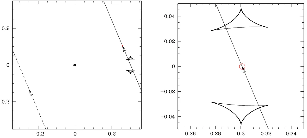
Figure 5.MOA-2010-BLG-117 caustic configuration with the source trajectories shown as the solid and dashed curves for sources 1 and 2, respectively. The arrows give the direction of motion for the sources with respect to the lens system, and the red circle indicates source star 1.

Table 2

MCMC Parameter Distributions

Parameter Units u0>0 u0<0

tE days 120.6(5.2) 116.4(4.3)

t0 HJD−2455400 19.80(30) 19.77(28)

u0 L 0.279(15) −0.287(13)

s L 0.8601(60) 0.8566(51)

θ radians 1.963(11) −1.964(10)

q 10−3 _{0.950(33) 0.952(33)}

t_* days 0.361(30) 0.372(29)

πE,N L −0.171(20) 0.188(22)

πE,E L −0.022(8) −0.040(10)

πE L 0.172(21) 0.192(23)

t0 2s HJD−2455400 −0.08(60) 0.22(9)

u0 2s L −0.267(19) 0.301(19)

fs I2 L 0.663(96) 0.731(92)

fs V2 L 0.801(117) 0.877(113)

dtEs2 days −1.2(11.6) −8.2(8.5)

dqs2 radians 0.305(35) −0.300(39)

ω 10−3days−1 0.79(1.21) −1.17(1.17)

s˙ 10−3days−1 −1.76(30) −1.76(30)

T

1 Sorb 10−3days−1 0.50(13) 0.49(12)

E

q mas 0.805(100) 0.777(95)

rel,G

m mas yr−1 2.46(31) 2.44(31)

Vs1 L 20.43(7) 20.38(6)

Is1 L 17.95(7) 17.90(6)

Ks1 L 14.90(8) 14.85(7)

Vs2 L 20.69(11) 20.53(10)

Is2 L 18.41(11) 18.25(10)

Ks2 L 15.58(14) 15.42(14)

Ks12 L 14.43(4) 14.34(4)

Irc0=14.288 and Vrc0-Irc0=1.06, which is appropriate

(Bensby et al. 2013; Nataf et al. 2013) for the Galactic coordinates of this event, (l, b)=(5.5875,−2.4680). This yields extinction values ofAI=1.580 andAV=2.995, which

implies an extinction-corrected primary source magnitude and colors ofIs1,0=16.421andVs1,0-Is1,0=1.052for the best-fit

model.

These dereddened magnitudes can be used to determine the angular source radius,θ_*. We use the relation from the analysis of Boyajian et al.(2014), but with a restricted range of colors corresponding to 3900<Teff<7000 K (T. Boyajian 2014,

private communication). We use

V I I

log 2 1mas

0.501414 0.419685 s 0.2 s , 5

10

1,0 1,0

* q

= + -

-[ ( )]

( ) ( )

and this givesθ_*=2.20μas for the best-fit model. Now, there is some indication of differential reddening in the CMD (Figure 7), so this can add some uncertainty to our determination of θ_*. Fortunately, the effect of this uncertainty in the extinction tends to cancel contributions from(V-I)s1,0

and Is1,0 in Equation(5). To account for this uncertainty, we

add a 13% uncertainty to our extinction estimates, which translates into a 9% uncertainty in θ_*, according to

Equation (5), to be used in our MCMC calculations. As Figure7indicates, the uncertainty in the magnitude and color of source 1 is larger than the uncertainty for most events. This is because flux can be traded between the two sources. However, this source radius determination is correlated with the other microlens model parameters, particularly the Einstein radius crossing time, tE, which occurs in the qE =q_*tE t_* formula. Therefore, we determine θE for each model in our

MCMC, and this yields the qE values listed in Table 2: θE=0.805±0.100 mas for the u0>0 solutions and

θE=0.777±0.095 mas for theu0<0solutions.

5. Lens System Properties

When both the angular Einstein radius, qE, and the microlensing parallax, pE, are measured, we can use the following relation (Gould 1992; An et al. 2002; Gould et al.2004),

M c

G M

au

4 8.1439 mas , 6

L E

E

E

E

2

q p

q p

= = 

( ) ( )

to determine the mass of the lens system, but in our case, we have degenerate solutions to consider. The degeneracy

Figure 6.Correlations from our MCMC runs between lens velocity parameters(vsepandω)and the parameters that affect the inferred host star mass:dq,t*,tE,πE, and

dtE21, from our MCMC runs. Smallert*values imply largerθEvalues, which imply tighter constraints on the parameters that describe the source velocities,dθ, and

dtE21. Black, red, green, blue, magenta, and cyan indicate models that haveχ2values larger than the best-fit model byΔχ2<1, 1<Δχ2<4, 4<Δχ2<9,

allowing differentt_*values is probably unique to the specific circumstances of this event. However, the degeneracy between theu0>0andu0<0 solutions is a very common degeneracy

due to the reflection of the lens plane with respect to the orientation of the Earth’s orbit, which allows us to measure the parallax effect with ground-based data. For high-magnification events, the lens–source system has an approximate reflection symmetry, so this u0>0«u0 <0 degeneracy has little

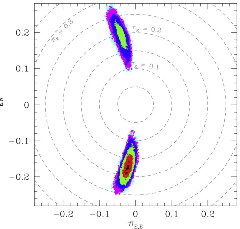
effect on pEº∣pE∣. Because the binary source system for MOA-2010-BLG-117 has u0» -u0 2s and source 2 is only ∼0.3 mag fainter than source 1, the lens-and-source system in this event also has an approximate symmetry(assuming that the planetary feature has little influence on the microlensing parallax signal). This could be the reason why the distributions of thepEvector, shown in Figure8, also show this approximate reflection symmetry. This figure shows the distributions from both degenerate solutions with best-fit parameters listed in Table1and Markov chain distributions listed in Table 2. The

u0>0 and u0<0 solutions are widely separated with

opposite signs for the π_E,Nvalues. These opposite signs mean

that the∣pE N, ∣values are very similar for all solutions. TheπE,E

values are also similar and much smaller than∣pE N, ∣, so theπE

values for all the degenerate solutions are similar. This means that there is overlap in the mass distributions predicted by all four degenerate solutions.

As mentioned in Section 3, we impose a requirement that both sources lie on the same isochrone. This requirement is not

imposed during the light curve modeling, but it is imposed in our Bayesian analysis that uses all of the models from our Markov chains to determine the physical parameters of the lens system. Each light curve model in our Markov chains is weighted by the _c2 _{of the best fit of the model source}

magnitudes and colors to the isochrones. Thus, the location of the source magnitudes and colors in Figure7does not depend on these isochrones, but the color-coding of the source magnitudes and colors does depend on the depend on the fit to the isochrones. We use isochrones from the PAdova and TRieste Stellar Evolution Code (PARSEC) project (Bressan et al.2012; Chen et al.2014,2015; Tang et al.2014). Wefind that our modeling results are consistent with isochrones with ages in the range of 4–10 Gyr and metallicity in the range of −0.04„[Fe/H]„0.58. These values are quite typical of Galactic bulge stars, as indicated by the microlens source stars with high-resolution spectra taken at high magnification by Bensby et al.(2013,2017). However, it is also possible that the source might have a slightly higher extinction than the average of the red clump stars. In that case, the range of allowed source star metallicities might extend to subsolar metallicities.

The main practical effect of this isochrone constraint is to force the source star system to be located on the near side of the bulge. The isochrones prefer a source distance of DS=

6.21.1 kpc, but when these priors on the source density

and microlensing probability are included, this shifts to

DS=6.9±0.7 kpc, as given in Table3.

We determine the physical parameters of this lens system with a Bayesian analysis marginalized over the Galactic model used by Bennett et al. (2014), and the results are summarized in Figures9and10, as well as in Table3. The host star and planet masses(Mhand mp) are determined directly from Equation(6)

with theπ_E,q, source magnitude, and color values determined for each model in our MCMC. Theθ_*andθ_Evalues are determined

Figure 7. (V-I I, ) color–magnitude diagram (CMD) of the stars in the OGLE-III catalog(Szymański et al.2011)within 90″of MOA-2010-BLG-117. The red spot indicates the red clump giant centroid, and the smaller spots of different colors indicate the magnitude and colors of the two sources from our MCMC calculations. Red, green, blue, magenta, and cyan indicate models that have χ2 values larger than the best-fit model by Δχ2<1, 1<Δχ2<4, 4<Δχ2_{<9, 9<Δχ}2_{<16, and 16<Δχ}2_{, respectively. Source 1 is}

brighter and redder than source 2 for most models. The gray line indicates the isochrone that best matches the source magnitudes and colors of the best-fit model. This isochrone has an age of 4.0 Gyr and a metallicity of [Fe/H]=0.28.

Figure 8.Values of the microlensing parallax vector,pE, from our MCMC runs are shown. Theu0>0 solutions haveπE,N<0 and are preferred over the

u0<0 solutions(withπE,N>0)byΔχ

2

=9.17. The MCMC points are color-coded. The points within Δχ2_{<1 are black, and the points within}

1_{< Dc}2_<4_{, 4<Δχ}2

<9, 9<Δχ2<16, 16<Δχ2<25, and 25<Δχ2_{are red, green, blue, magenta, and cyan, respectively. The dashed}

circles indicate curves of constantπE.

directly from Equations (5), (3), and (4) for each model. The

u0<0 solutions are weighted bye_-Dc2 2₌0.122

with respect to theu0>0 solutions, whereΔχ2=4.21 is the χ2difference between the best-fit solutions with the parameters listed in Table1. There is no appreciable difference in the parameter space volume covered by the two solutions, so this approach is adequate. The Galactic model prior has little influence on the lens mass determination because the prior has little variation over the parameter values that are consistent with the MCMC light curve models. The Galactic model has a larger influence on the distance to the lens, because the stellar density has a strong dependence on the distance to the source star, DS. The relation between the

distances to the lens and source stars is given by

DL au , 7

E E S

p q p =

+ ( )

where π_S is the parallax of the source star, π_S=au/DS. As

Table3 indicates, these calculations indicate that the host star has a mass ofMh=0.58±0.10Meand the planet has a mass

of Mp=0.51±0.07MJup, whereMJupis the mass of Jupiter.

Assuming a random orientation, their three-dimensional separation isa3d 2.9

1.6 0.5

= +_- au. The planet mass uncertainty is smaller than the host mass uncertainty because the high host star mass(t_*<0.34 days),u0>0 solutions have a lower mass ratio than the other solutions, as indicated in Tables 1and 2.

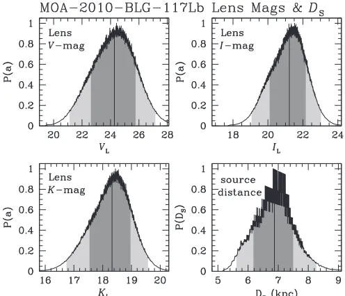
The predicted host(and lens)starV,I, andKmagnitudes are shown in Figure 10, along with the source distance,DS. The

distribution ofDSfavors a large number of discrete values. This

is due to our requirement that the two source stars lie on the same isochrone and the discrete values of the metallicity, [Fe/H], andlog Age( )at intervals of 0.04 and 0.05, respectively. The additional source star also increases our odds of detecting planets orbiting the lens star because the second source provides a second probe of the lens plane. This can be seen in Figure11, which shows the two cases from our recent exoplanet mass ratio function paper(Suzuki et al.2016). Over much of the parameter range, the second source star approximately doubles the planet detection efficiency. How-ever, this is a much smaller increase than is provided by high-magnification events.

6. Keck Follow-up Observations

In an attempt to identify the lens and planetary host star, we have obtained high angular resolution AO observations from the Keck II telescope. Unfortunately, the seeing conditions

were relatively poor compared to some of our other Keck observations(Batista et al.2015)that achieved a point-spread function(PSF)FWHM of 60 mas. Our stackedK-band image

of the MOA-2010-BLG-117 field has a PSF FWHM of

220 mas, and it is shown in Figure12. The Keck images were taken in 2012, two years after the event. With a lens–source relative proper motion ofmrel,G=2.450.31 mas yr-1, there

is no chance to detect the lens–source separation either through image elongation (Bennett et al. 2007, 2015) or a color-dependent image centroid shift(Bennett et al.2006). However, there is still a chance to detect the unresolved lens starflux on top of theflux from the source stars. In this case, the source stars are relatively bright subgiants, so it would be difficult to detect a host star as faint as the star indicated by the finite

Table 3

Physical Parameters

Parameter Units Value 2-σrange

DS kpc 6.9±0.7 5.6–8.3

DL kpc 3.5±0.4 2.9–4.3

Mh Me 0.58±0.11 0.39–0.83

mp MJup 0.54±0.10 0.38–0.77

a⊥ au 2.42±0.26 1.93–2.97

a3d au 2.9

1.6 0.6

+

- 2.1–10.3

VL mag 24.3-+1.71.5 21.1–27.2

IL mag 21.2-+1.11.0 19.1–23.0

KL mag 18.3-+0.80.6 16.7–19.6

Note.Uncertainties are 1σparameter ranges.

Figure 9.Probability distributions of the planet and host star mass, three-dimensional separation and lens system distance based on a Bayesian analysis using mass and distance determinations from the MCMC light curve distributions along with prior probabilities from a standard Galactic model.

source and microlensing parallax measurements, as discussed in Section5.

The “star” detected in the Keck AO images is indeed significantly brighter, KKeck=13.97±0.04, than the com-bined flux of the source stars, which is Ks12=14.43±0.04.

However, this excess blendflux atKb=15.12±0.15 does not

match the lens mass and distance derived in Section 5. The

predicted host star brightness is KL 18.3 0.8 0.6

= _-+ _{, and as can be}

seen from Figure10, the probability of the lens(and host)star being brighter thanKL<16 is negligible. Figure13compares

the constraints from the microlensing parallax, angular Einstein

Figure 11.Planetary detection efficiency for MOA-2010-BLG-117. The left panel shows the detection efficiency due to the source star that led to the real planet detection, and the right panel shows the planet detection efficiency for the actual event with both source stars. In both cases, the black spots indicate the position of the planet.

Figure 12. Co-added Keck AO image of the target star indicated by the crosshairs. The target consists of the combinedflux of the source stars, the lens

(and planetary host star), any bound companions to either the source or lens system, and possibly an unrelated star that happens to be located0 2 from the source.

Figure 13.Constraints on the host star mass and distance from the microlensing parallax,πE(in blue), the angular Einstein radius,θE(in red), and the host star

flux(in green), under the assumption that the excessflux observed in the Keck AO images is due to the host star. The dashed line indicates the approximate 1σ uncertainty contours(which ignore the correlations between the parameters). For the excessK-bandflux, the solid green line is from a 5 Gyr isochrone and the dashed green lines represent 3 and 7 Gyr isochrones(Bressan et al.2012; Chen et al.2014,2015; Tang et al.2014).

radius, and lensflux constraints, assuming that the excessflux is due to the lens star. Obviously, these constraints are not consistent with each other. The most likely solution to this inconsistency is simply that the excess flux is not due to the lens. The other possibilities that could explain this excessflux at the position of the source star are a binary companion to the lens, a tertiary companion to the source stars, or an unrelated star. A Bayesian analysis using the measured bulge luminosity function and measured frequencies of multiple star systems (N. Koshimoto et al. 2017, in preparation) gives similar probabilities for each of these possibilities, with slightly larger probabilities for lens and source companions than for an unrelated star.

Although we believe that the result from the π_E and θ_E measurements is very likely to be the correct interpretation, we will briefly consider that one of these measurements is wrong. From Figure13, we see that a host star mass ofMh∼1Meat a

distance ofDL∼2.6 kpc would be favored if the blendflux is

due to the lens star and the π_E measurement is correct. Alternatively, if thepE measurement were incorrect, while the θEmeasurement were correct and the blendflux were due to the

lens star, then the lens star would have to be an evolved star above a solar mass. The green isochrone curves in Figure 13

are nearly horizontal where they cross the red qE=const.

curve. This is due to the fact that stars evolve very quickly through these evolved phases, and this implies that this solution is particularly unlikely.

A final possibility is that the π_E and θ_E measurements are correct, and that the excessflux comes from the planetary host star. This would imply that the assumption made for the red and blueθ_Eandπ_Ecurves in Figure13that the source is in the Galactic bulge (at DS =6.80.6 kpc) is not correct. From

Equation (7), we have DS=DL (1-p qE EDL au), and this

tells us that if the lens system is located atDL≈0.9 where the

green lens flux curve crosses the Mh=0.580.10 value

indicated by the θE and πE measurements (according to

Equation (6)), then the source would be at a distance of

DS=1.04 kpc. This is highly unlikely or at least ruled out for

two reasons. First, the rate that stars at this distance are microlensed is more than two orders of magnitude lower than the rate that bulge stars are microlensed. Second, the two source stars appear to reside on the Galactic bulge subgiant branch of the CMD, shown in Figure7. Very few foreground disk stars lie on this portion of the CMD, and there is virtually no way to arrange for the fainter star in a binary pair to be bluer than the brighter star.

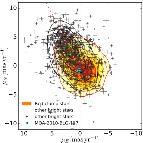
Another indication that the source stars must reside in the Galactic bulge comes from the proper motion of the source star system. Skowron et al. (2014) has developed a method to determine the proper motion of microlens source stars in the presence of a modest amount of blending with other stars. We have used this method to measure the proper motions of stars brighter than I<17.87, for just over five years of OGLE-IV data. (This magnitude cut is two magnitudes below the red clump centroid.)Figure14shows that the proper motion of the target, consisting of the two source stars and a blend star with a magnitude of about the average of the two source stars. If the blend star were the lens, it would be in the Galactic disk, so we would expect the average proper motion of the two source stars and the blend to be shifted slightly in the direction of the disk rotation(given by the dashed white line in the NNE direction). Instead, we find the proper motion of the target to be

, 0.15 0.34, 0.81 0.36 mas yr

E E, E N, 1

m m =  - 

-( ) ( ) .This

clearly indicates that the target is unlikely to be in the disk. Of course, it could be that the blend star and the two source stars are not in the same population, and their proper motions could partially cancel. However, our light curve modeling indicates that the lens–source relative proper motion is in the range of 2–3 mas yr−1, so if the blend star were the lens, its proper motion could be at most∼1 mas yr−1in the direction of disk rotation. Thus, it would not have disk kinematics. This tends to confirm our conclusion that the blend star cannot be the lens. So, we conclude that the source star system resides in the Galactic bulge and that the host star mass and the lens system distance are determined by the π_E and θ_E measurements, as described in Section5.

7. Discussion and Conclusions

We have presented the first planetary microlensing event with two magnified source stars. This event has an obvious planetary feature, but it could not be modeled with a single source star microlensed by a lens system consisting of one star and one planet. The basic properties of the planetary feature could be explained by models with two source stars or else a circumbinary planet. The choice between these two options was delayed by early difficulties in modeling the event. These difficulties were overcome by adding the requirement that the

flux ratio between the two sources be consistent with different passbands to allow the best light curve model to be found much more easily. Thefinite source effects and microlensing parallax

signal indicate that the planet and host have masses of

mp=0.58±0.10MJupand Mh=0.51±0.07 Me at a two-dimensional separation ofa⊥=2.44±0.26 au and a distance

of DL=3.40.2 kpc. This is a Jupiter-mass-ratio planet

orbiting at about twice the distance of the snow line, which is similar to Jupiter’s orbit.

One complication in the interpretation of this event is the

K-band Keck AO images that indicate an excess of flux at the location of the source. This excessflux is much brighter than the brightness expected from the lens star, based on the mass determined from theθ_Eandπ_Emeasurements. We consider the possibility that this excessflux could be due to the lens, but we

find that the excessflux is more likely to be due to a companion to the lens star, the source stars, or an unrelated star. This is not thefirst planetary microlensing event with a binary source star, as the planetary event OGLE-2007-BLG-368(Sumi et al.2010)

has a binary source star that was revealed via the xallarap effect. (Xallarap is the effect of source orbital motion on the microlensing light curve.)

This event was as challenging to model as events with an additional lens mass, either a second star (Gould et al. 2014; Poleski et al. 2014; Bennett et al. 2016) or a second planet (Gaudi et al. 2008; Bennett et al. 2010; Han et al. 2013; Beaulieu et al.2016). However, events with an additional lens mass have interesting implications regarding the properties of exoplanet systems, while events with two source stars do not. The only advantage of a second source star is a modest increase in the exoplanet detection efficiency. Nevertheless, microlen-sing is currently our best method for understanding the population of exoplanets that orbit beyond the snow line, and the statistical analysis of the planet populations probed by the microlensing method requires that the correct microlensing model be found for all planetary microlensing events. The new method that we have presented in this paper aids in this effort, and it has enabled the MOA Collaboration analysis that has discovered a break in the exoplanet mass ratio function(Suzuki et al.2016).

D.P.B., A.B., and D.S. were supported by NASA through grant NASA-NNX12AF54G. This work was partially sup-ported by a NASA Keck PI Data Award, administered by the NASA Exoplanet Science Institute. Data presented herein were obtained at the W. M. Keck Observatory from telescope time allocated to the National Aeronautics and Space Administration through the agency’s scientific partnership with the California Institute of Technology and the University of California. The Observatory was made possible by the generous financial support of the W. M. Keck Foundation. The OGLE Team thanks Profs. M. Kubiak and G. Pietrzyński for their contribution to the collection of OGLE photometric data. The OGLE project has received funding from the National Science Centre, Poland, grant MAESTRO 2014/14/A/ST9/00121 to A.U. The work by C.R. was supported by an appointment to the NASA Postdoctoral Program at the Goddard Space Flight Center, administered by USRA through a contract with NASA. The work by N.K. is supported by JSPS KAKENHI Grant Number JP15J01676. A.G. and B.S.G. were supported by NSF grant AST 110347 and by NASA grant NNX12AB99G.

ORCID iDs

D. P. Bennett https://orcid.org/0000-0001-8043-8413

C. Han https://orcid.org/0000-0002-2641-9964

J.-P. Beaulieu https://orcid.org/0000-0003-0014-3354

J. Skowron https://orcid.org/0000-0002-2335-1730

B. S. Gaudi https://orcid.org/0000-0003-0395-9869

N. Koshimoto https://orcid.org/0000-0003-2302-9562

A. Fukui https://orcid.org/0000-0002-4909-5763

Y. Itow https://orcid.org/0000-0002-8198-1968

N. J. Rattenbury https://orcid.org/0000-0001-5069-319X

D. Suzuki https://orcid.org/0000-0002-5843-9433

R. W. Pogge https://orcid.org/0000-0003-1435-3053

J. C. Yee https://orcid.org/0000-0001-9481-7123

M. D. Albrow https://orcid.org/0000-0003-3316-4012

E. Bachelet https://orcid.org/0000-0002-6578-5078

V. Batista https://orcid.org/0000-0002-9782-0333

J. A. R. Caldwell https://orcid.org/0000-0002-3861-5241

K. Horne https://orcid.org/0000-0003-1728-0304

M. Hundertmark https://orcid.org/0000-0003-0961-5231

N. Kains https://orcid.org/0000-0001-8803-6769

S. R. Kane https://orcid.org/0000-0002-7084-0529

K. C. Sahu https://orcid.org/0000-0001-6008-1955

J. Wambsganss https://orcid.org/0000-0002-8365-7619

References

Albrow, M. D., et al. 2009,MNRAS,397, 2099

Alcock, C., Allsman, R. A., Alves, D., et al. 1995,ApJL,454, L125

An, J. H., Albrow, M. D., Beaulieu, J.-P., et al. 2002,ApJ,572, 521

Batista, V., Beaulieu, J.-P., Bennett, D. P., et al. 2015,ApJ,808, 170

Beaulieu, J.-P., Bennett, D. P., Batista, V., et al. 2016,ApJ,824, 83

Bennett, D. P. 2008, in Exoplanets, ed. J. Mason (Berlin: Springer)

(arXiv:0902.1761)

Bennett, D. P. 2010,ApJ,716, 1408

Bennett, D. P., Anderson, J., Bond, I. A., Udalski, A., & Gould, A. 2006,

ApJL,647, L171

Bennett, D. P., Anderson, J., & Gaudi, B. S. 2007,ApJ,660, 781

Bennett, D. P., Batista, V., Bond, I. A., et al. 2014,ApJ,785, 155

Bennett, D. P., Bhattacharya, A., Anderson, J., et al. 2015,ApJ,808, 169

Bennett, D. P., Bond, I. A., Udalski, A., et al. 2008,ApJ,684, 663

Bennett, D. P., & Rhie, S. H. 1996,ApJ,472, 660

Bennett, D. P., & Rhie, S. H. 2002,ApJ,574, 985

Bennett, D. P., Rhie, S. H., Nikolaev, S., et al. 2010,ApJ,713, 837

Bennett, D. P., Rhie, S. H., Udalski, A., et al. 2016,AJ,152, 125

Bennett, D. P., Sumi, T., Bond, I. A., et al. 2012,ApJ,757, 119

Bensby, T., Feltzing, S., Gould, A., et al. 2017, arXiv:1702.02971

Bensby, T., Yee, J. C., Feltzing, S., et al. 2013,A&A,549, A147

Bertelli, G., Girardi, L., Marigo, P., & Nasi, E. 2008,A&A,484, 815

Bond, I. A., Abe, F., Dodd, R. J., et al. 2001,MNRAS,327, 868

Borucki, W. J., Koch, D. G., Basri, G., et al. 2011,ApJ,736, 19

Boyajian, T. S., van Belle, G., & von Braun, K. 2014,AJ,147, 47

Bressan, A., Marigo, P., Girardi, L., et al. 2012,MNRAS,427, 127

Burke, C. J., Christiansen, J. L., Mullally, F., et al. 2015,ApJ,809, 8

Cassan, A., Kubas, D., Beaulieu, J.-P., et al. 2012,Natur,481, 167

Chen, Y., Bressan, A., Girardi, L., et al. 2015,MNRAS,452, 1068

Chen, Y., Girardi, L., Bressan, A., et al. 2014,MNRAS,444, 2525

Gaudi, B. S. 2012,ARA&A,50, 411

Gaudi, B. S., Bennett, D. P., Udalski, A., et al. 2008,Sci,319, 927

Gould, A. 1992,ApJ,392, 442

Gould, A. 2008,ApJ,681, 1593

Gould, A., Bennett, D. P., & Alves, D. R. 2004,ApJ,614, 404

Gould, A., Dong, S., Bennett, D. P., et al. 2010a,ApJ,710, 1800

Gould, A., Dong, S., Gaudi, B. S., et al. 2010b,ApJ,720, 1073

Gould, A., Gaudi, B. S., & Han, C. 2004, arXiv:astro-ph/0405217

Gould, A., & Loeb, A. 1992,ApJ,396, 104

Gould, A., Udalski, A., Shin, I.-G., et al. 2014,Sci,345, 46

Han, C., Bennett, D. P., Udalski, A., et al. 2016,ApJ,825, 8

Han, C., Udalski, A., Choi, J.-Y., et al. 2013,ApJL,762, L28

Han, C., Udalski, A., Gould, A., et al. 2017,AJ,154, 223

Hwang, K.-H., Choi, J.-Y., Bond, I. A., et al. 2013,ApJ,778, 55

Ida, S., & Lin, D. N. C. 2005,ApJ,626, 1045

Jung, Y. K., Udalski, A., Yee, J. C., et al. 2017,AJ,153, 129

Kennedy, G. M., & Kenyon, S. J. 2008,ApJ,673, 502

Kennedy, G. M., Kenyon, S. J., & Bromley, B. C. 2006,ApJL,650, L139

Kervella, P., Thévenin, F., Di Folco, E., & Ségransan, D. 2004,A&A,426, 297

Lecar, M., Podolak, M., Sasselov, D., & Chiang, E. 2006,ApJ,640, 1115

Lissauer, J. J. 1993,ARA&A,31, 129

Mao, S., & Paczyński, B. 1991,ApJL,374, L37

Minniti, D., Lucas, P. W., Emerson, J. P., et al. 2010,NewA,15, 433

Mullally, F., Coughlin, J. L., Thompson, S. E., et al. 2016, arXiv:1602.03204

Muraki, Y., Han, C., Bennett, D. P., et al. 2011,ApJ,741, 22

Nataf, D. M., Gould, A., Fouqué, P., et al. 2013,ApJ,769, 88

Pejcha, O., & Heyrovský, D. 2009,ApJ,690, 1772

Poleski, R., Skowron, J., Udalski, A., et al. 2014,ApJ,795, 42

Pollack, J. B., Hubickyj, O., Bodenheimer, P., et al. 1996,Icar,124, 62

Rhie, S. H., Becker, A. C., Bennett, D. P., et al. 1999,ApJ,522, 1037

Schechter, P. L., Mateo, M., & Saha, A. 1993,PASP,105, 1342

Skowron, J., Udalski, A., Szymański, M. K., et al. 2014,ApJ,785, 156

Spergel, D., Gehrels, N., Baltay, C., et al. 2015, arXiv:1503.03757

Sumi, T., Bennett, D. P., Bond, I. A., et al. 2010,ApJ,710, 1641

Suzuki, D., Bennett, D. P., Sumi, T., et al. 2016,ApJ,833, 145

Szymański, M. K., Udalski, A., Soszyński, I., et al. 2011, AcA,61, 83

Tang, J., Bressan, A., Rosenfield, P., et al. 2014,MNRAS,445, 4287

Thommes, E. W., Matsumura, S., & Rasio, F. A. 2008,Sci,321, 814

Tomaney, A. B., & Crotts, A. P. S. 1996,AJ,112, 2872

Twicken, J. D., Jenkins, J. M., Seader, S. E., et al. 2016,AJ,152, 158

Udalski, A. 2003, AcA,53, 291

Udalski, A., Jung, Y. K., Han, C., et al. 2015a,ApJ,812, 47

Udalski, A., Szymański, M., Kałużny, J., et al. 1994, AcA,44, 227

Udalski, A., Szymański, M. K., & Szymański, G. 2015b, AcA,65, 1