Traveltime and conversion-point computations and parameter estimation in layered, anisotropic media by tau-p transform

This is a repository copy of

Traveltime and conversion-point computations and parameter

estimation in layered, anisotropic media by tau-p transform

.

White Rose Research Online URL for this paper:

http://eprints.whiterose.ac.uk/327/

Article:

Van der Baan, M. and Kendall, M.J. (2003) Traveltime and conversion-point computations

and parameter estimation in layered, anisotropic media by tau-p transform. Geophysics,

68 (1). pp. 210-224. ISSN 0016-8033

https://doi.org/10.1190/1.1543208

[email protected]

https://eprints.whiterose.ac.uk/

Reuse

See Attached

Takedown

If you consider content in White Rose Research Online to be in breach of UK law, please notify us by

GEOPHYSICS, VOL. 68, NO. 1 (JANUARY-FEBRUARY 2003); P. 210–224, 8 FIGS., 2 TABLES. 10.1190/1.1543208

Traveltime and conversion-point computations and parameter

estimation in layered, anisotropic media by

τ

-

p

transform

Mirko van der Baan

and J.-Michael Kendall

ABSTRACT

Anisotropy influences many aspects of seismic wave propagation and, therefore, has implications for con-ventional processing schemes. It also holds information about the nature of the medium. To estimate anisotropy, we need both forward modeling and inversion tools. For-ward modeling in anisotropic media is generally done by ray tracing. We present a new and fast method using theτ-ptransform to calculate exact reflection-moveout curves in stratified, laterally homogeneous, anisotropic media for all pumode and converted phases which re-quires no conventional ray tracing. Moreover, we obtain the common conversion points for both P-SV and P-SH converted waves. Results are exact for arbitrary strength of anisotropy in both HTI and VTI media (transverse isotropy with a horizontal or vertical symmetry axis, respectively).

Since inversion for anisotropic parameters is a highly nonunique problem, we also develop expressions de-scribing the phase velocities that require only a reduced number of parameters for both types of anisotropy. Nev-ertheless, resulting predictions for traveltimes and con-version points are generally more accurate than those obtained using the conventional Taylor-series expan-sions. In addition, the reduced-parameter expressions are also able to handle kinks or cusps in the SV trav-eltime curves for either VTI or HTI symmetry.

INTRODUCTION AND MOTIVATION

In anisotropic media, many wave phenomena occur which are counterintuitive to our conception of isotropic wave mo-tion. To account for these effects, successful data processing requires a high level of knowledge concerning the way partic-ular anisotropy parameters affect the data. To a certain extent,

Published on Geophysics Online July 19, 2002, Manuscript received by the Editor August 22, 2001; revised manuscript received May 24, 2002. ∗_{University of Leeds, School of Earth Sciences, Woodhouse Lane, Leeds LS2 9JT, United Kingdom. E-mail: [email protected];}

[email protected]. c

°2003 Society of Exploration Geophysicists. All rights reserved.

insights can be gained through analytical treatments and for-ward modeling tools (e.g., by means of ray tracing). However, ultimately we need to assess the actual anisotropy parameters in a certain region. We therefore require accurate inversion tools. Furthermore, given the ever increasing size of data vol-umes, any modeling and inversion tools should be both fast and easy to implement.

In this paper, we extend the results of Van der Baan and Kendall (2002; hereafter, paper I), who demonstrated how the

τ-ptransform can be used both as a forward modeling tool to compute exact moveout curves of pure-mode data (e.g., P-P reflections) and as an inversion tool to extract the anisotropy parameters in transversely isotropic media with a vertical sym-metry axis (VTI). We extend these results to also incorporate transversely isotropic media with a horizontal symmetry axis (HTI) and converted waves (e.g., P-SV reflections). In addi-tion, this method can be used to calculate exact common con-version points in both symmetries for all offsets and azimuths. Finally, approximate solutions for the conversion points using a reduced set of parameters are also determined which are more suitable for inversion.

Conventionally, within the limit of ray theory, exact trav-eltimes and conversion points are calculated by means of ray-tracing methods (Gajewski and Pˇsenˇc´ık, 1987; Kendall and Thomson, 1989). Unfortunately, their implementation is rather involved, even for simple laterally homogeneous media. Fur-thermore, their extension to a complete anisotropic tomogra-phy approach in 3D is also rather prohibitive [see, for instance, Chapman and Pratt (1992) for a 2D approach].

Another method for solving the forward problem is to use Taylor-series expansions (Tsvankin and Thomsen, 1994; Alkhalifah and Tsvankin, 1995; Al-Dajani and Tsvankin, 1998; Thomsen, 1999). However, this does not yield exact results, and their applicability is currently limited to VTI media for converted-wave phases (Tsvankin and Thomsen, 1994). For pure-mode data, expressions for orthorhombic media exist (Al-Dajani et al., 1998; Al-Dajani and Toks ¨oz, 1999). In paper I, we demonstrated that the traveltime predictions of the τ-p method using reduced-parameter

expressions are more accurate than those of the conven-tional Taylor-series approach for VTI media. In this paper, we show that this is even more true for the predictions of the conversion points of P-SV converted waves in VTI me-dia. Furthermore, contrary to the Taylor-series approach, our method is easily extended to also handle converted-wave trav-eltimes and common conversion points in, for instance, HTI media.

As an introduction, we illustrate the effects of anisotropy on traveltimes and conversion points using a simple model comprised of two layers over a half space. The upper layer is 500-m thick, isotropic, and hasα0=1.8 km/s andβ0=1.0 km/s

for the P- and S-wave velocities, respectively. The second layer is also 500 m thick and has isotropic background ve-locities of α0=2.5 km/s and β0=1.4 km/s. Four models of

anisotropy in the second layer are considered: (1) isotropy, (2) VTI anisotropy with Thomsen (1986) parameters ǫ, γ,

δ=0.05 (elliptic anisotropy), (3) fluid (water)-filled fractures, and (4) gas-filled fractures. The fractures are vertically aligned

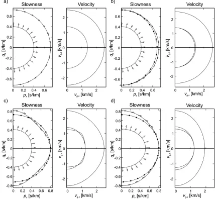
FIG.1. Vertical slices of the slowness surfaces (left side) and wave surfaces (right side) for the second layer in four models. The particle motion for each wavesheet is indicated by vectors on the slowness surfaces. (a) Isotropic model, (b) transversely isotropic with a vertical symmetry axis (VTI), (c) vertically aligned fluid-filled fractures, (d) vertically aligned gas-filled fractures. The fracture density is 0.1, the aspect ratio is 0.001, and the normal to fracture plane is in the offset directionx. The anisotropic models display rotational symmetry around, respectively, the vertical (b) and horizontal axis [(c) and (d)].

(HTI media) with the normal to the crack face oriented in the offset direction. The crack density is 0.1, the crack aspect ratio is 0.001, and the theory of Hudson (1981) is used to con-struct effective-medium models. The traveltimes and raypaths in these media have been computed using the exact ray tracer ATRAK (Guest and Kendall, 1993). Figure 1 shows the slow-ness and wave surfaces for the four cases. Note that the P-wave velocity surfaces show a 180◦_{periodicity in the gas-filled case} and a 90◦_{periodicity in the fluid-filled case.}

Large differences occur in the converted-wave raypaths and therefore the conversion-point distributions. Figure 3 shows raypaths for P-wave reflections from the base of layer 2 at offsets of 200 and 900 m, and the associated P-SV converted waves. The four cases show large variations in converted-wave raypaths for constant P-wave emergence offset. In the fracture cases, there is little variation between the P- and SV-wave ray-paths through the anisotropic layer which leads to converted-wave offsets which are very near the P-converted-wave emergence offsets. Although the wavefront normals (i.e., the plane-wave propaga-tion direcpropaga-tions) are very different for the P- and SV-waves, the group velocities and therefore the raypaths are nearly aligned, especially in the fluid-filled fracture case. The large differences in converted-wave emergence offsets suggest that the actual location of the conversion point is very sensitive to the under-lying cause of anisotropy. Therefore, accurately assessing the anisotropy parameters in a particular area is very important be-fore data can be successfully sorted into common-conversion-point gathers.

In this paper, we first review the equations describing the form of theτ(pr) curves. Next, we develop the required

ex-pressions for the phase velocities as a function of horizontal slowness in both HTI and VTI media, and we show how exact traveltime curves and conversion points can be computed in lat-erally homogeneous, layered media. We then derive reduced-parameter expressions which can be used in inversions for anisotropy parameters. Finally, a general inversion strategy is put forward, and we conclude with a numerical example using the elastic coefficients of a strongly anisotropic shale.

THEORY

Traveltimes and the slant stack

For an anisotropic earth composed of a stack of horizon-tal layers, Hake (1986) showed that there exists a direct link

FIG.2. Traveltimes for the four models: isotropic model (solid line), (elliptic) VTI model (long dashes), fluid-filled fractures (short dashes) and gas-filled fractures (dotted line).

between theτ-p transform and the traveltime curves of re-flections. Namely, the traveltimet(x,y) can be linearly decom-posed into

t= pxx+pyy+

X

i

zi( `qz,i+q´z,i)= pxx+pyy+τ, (1)

wherepxandpyrepresent the horizontal slowness in thex- and

y-directions, respectively;zithe thickness of layeri; `qz,iand ´qz,i the absolute vertical slowness of, respectively, the down- and upgoing plane waves in that layer; andτthe total intercept time.

Snell’s law, which states that the horizontal slowness compo-nents px andpyremain constant for horizontal layering, has been used to derive this exact equation. Theτ-ptransform can be identified in equation (1) sinceziq`z,i equals1τ`i, the one-way intercept time of the downgoing plane wave in layerifor a given slowness, and the two-way intercept times1τi add up linearly. That is,

X

i

zi( `qz,i+q´z,i)=

X

i

(1τ`i+1τ´i)=

X

i

1τi=τ. (2)

Hake’s (1986) result was originally formulated for a 2D medium. However, Diebold (1987) showed for the isotropic case that the relation between the traveltimes and theτ-p trans-form can be extended to three dimensions. This remains true for 3D anisotropic media.

To simplify the mathematical notation, we introduce the ra-dial slowness in the horizontal planepr=(px,py,0)twith mag-nitude|pr| =pr, and the emergence offsetr=(x,y,0)t at dis-tance |r| =r from the source. Hence, equation (1) simplifies to

t =pr·r+

X

i

zi( `qz,i+q´z,i)= prr+τ. (3)

Formulas (1)–(3) for theτ-ptransform remain valid regardless of the type of anisotropy and the type of waves (i.e., P, SV, SH). In order to calculate traveltime curves in layered anisotropic media using equation (3), we need a mathematical descrip-tion of theτ(pr) curves. For the downgoing waves, such an

expression can be derived using the fact that the one-way in-terval zero-offset traveltime,1t0`,i, equals the interval inter-cept time of the vertically downgoing wave, 1τ`0,i. That is,

1τ`0,i=1t`0,i=zi/v`0,i with `v0,i the phase velocity of the verti-cally downgoing wave. Hence,

1τ`i/1τ`0,i =

ziq`z,i

zi/v`0,i

=v`0,iq`z,i =v`0,i

£

`

v−_ph,i2 −p_r2¤1/2, (4)

with `vph,ithe phase velocity in layeri. A similar expression ex-ists for the upgoing waves. Therefore, the two-wayτ(pr) curves

are expressed by

1τi/1τ0,i=

(1τ`i+1τ´i)

(1τ`0,i+1τ´0,i)

= v`0,iv´0,i `

v0,i+v´0,i

[ `qz,i+q´z,i]

= v`0,iv´0,i `

v0,i+v´0,i

£¡

`

v−_ph,i2 −p_r2¢1/2

+¡v´−_ph,i2 −p_r2¢1/2¤, (5)

which follows from equations (2) and (4). Expression (5) can handle any type of anisotropy and all phases including con-verted waves. It simplifies if the phase velocity function of a pure-mode reflection is symmetric with respect to the horizon-tal plane, since in that case `qz,i=q´z,i=qz,i. Therefore, for pure-mode waves traveling in both HTI and VTI media, it reduces to (paper I)

1τi/1τ0,i =

v0,i

vph,i

£

1−p_r2v2_ph,i¤1/2. (6)

Expressions (5) and (6) describe the form of theτ(pr) curves.

To calculate the required traveltimes for a given slowness, both the exact phase velocities and the emergence offsetrare needed. These are derived in the next subsection.

Exact traveltimes and conversion points: Forward modeling

For general anisotropy and smoothly varying media, the Christoffel equation provides the phase velocities for a given plane-wave propagation direction (i.e., normal to wave front) [see, for instance, Auld (1973)]. The associated horizontal slow-nessprcan then be obtained by dividing the horizontal

compo-nent of the wavefront normalnrby the phase velocityvph. That

is,pr=nr/vph. Upon interaction with a horizontal interface,

the horizontal slownesspr of incident, transmitted, reflected,

and converted waves has to be preserved (Snell’s law). Un-fortunately, solving the Christoffel equation forprresults in a

sixth-order polynomial equation with possibly complex roots— a common problem while ray tracing in anisotropic structures (Gajewski and Pˇsenˇc´ık, 1987; Kendall and Thomson, 1989). We have to deal with a similar problem to compute the desired

τ(pr) curves.

On the other hand, for VTI, HTI, unrotated orthorhom-bic, and even unrotated monoclinic media, exact expressions for the phase velocities are known (Fryer and Frazer, 1987; Tsvankin, 1996, 1997a, b). In addition, these formulas can be expressed in terms of Thomsen’s (1986) parameters or gener-alizations thereof (Mensch and Rasolofosaon, 1997; Tsvankin, 1997a; Pˇsenˇc´ık and Gajewski, 1998) and finally be reordered such that they yield the exact phase velocity as a function of the horizontal slowness. Therefore, the desiredτ(pr) curves can be

computed analytically, thereby circumventing the problem of solving sixth-order polynomial expressions.

In HTI media, the common notation of SH and SV waves is not appropriate. We therefore change to the notation of Tsvankin (1997b). If we imagine that VTI symmetry is caused by fine-scale layering (isotropic horizontal layers) and HTI symmetry by parallel vertical cracks, then the symmetry axis is perpendicular to the layering and the crack planes, respec-tively. The S-phases polarized parallel to the layering are called Sk(previously SH) and the S-waves polarized within any plane containing the symmetry axis S⊥ (previously SV) since they are perpendicular to the layering [see Figure 1 in Tsvankin (1997b)]. Note that Crampin (1981) uses a similar definition. In his notation, SP corresponds to S⊥(SV) and SR to Sk(SH). The last two notations are unambiguous for both HTI and VTI symmetries. We will henceforth employ Tsvankin’s notation in terms of P, Sk, and S⊥.

In this new notation, phase velocities of respectively P- and

S⊥-waves in the crystallographic coordinate system of trans-versely isotropic media with a vertical symmetry axis are de-scribed by (Thomsen, 1986; Tsvankin, 1996)

v(_PT)(θ)=α₀(T)

·

1+ε(T)sin2θ−1 2f

(T)¡

1−

q

s_θ(T)¢

¸1/2

,

(7)

v_S(T)

⊥(θ)=α

(T) 0

·

1+ε(T)sin2θ−1 2f

(T)¡₁₊q_s(T)

θ

¢ ¸1/2

,

with

s_θ(T) =1+4 sin

2

θ f(T)

¡

2δ(T)cos2θ−ε(T)cos(2θ)¢

+4

£

ε(T)¤2_sin4_θ

£

f(T)¤2 , (9)

and

f(T)=1−£β₀(T)±α₀(T)¤2. (10)

The phase angleθrepresents the polar angle with the vertical axis. The quantitiesα(₀T),β₀(T),δ(T)_{, andε}(T) _{are the so-called}

generic Thomsen parameters withα(₀T)andβ₀(T)the phase ve-locities along the symmetry axis. The definitions ofδ(T)_andε(T)

are given in Thomsen (1986). The generic Thomsen parameters are defined in the so-called crystallographic coordinate system, which is independent of the global coordinate system (i.e., with respect to the earth’s surface). The appropriate expressions for Sk(SH) are contained in the Appendix.

VTI media.—For unrotated media, the crystallographic and the global coordinate systems are coincident. Therefore, the phase velocities in a VTI medium are also computed using

v(PT)(θ) andv

(T)

S⊥(θ), expressions (7) and (8). To distinguish these

parameters from an HTI medium, we use the superscript(v)_.

That is,

α₀(v)=α₀(T), β₀(v)=β₀(T),

δ(v)=δ(T)_{, . . .VTI}

ε(v)=ε(T), f(v)_{= f}(T)_.

(11)

Using Snell’s law,

pr =sin(θ)/vph, (12)

and reordering terms yields the required expressions for the phase velocity expressed as a function of the horizontal slow-ness. Hence,

v(_Pv)(pr)=α

(v) 0

×





2− f(v)+2¡

δ(v)f(v)−ε(v)¢£wα(v₀)

¤2

+ f(v)

q

s(pv)

2−4ε(v)£

wα(v₀)

¤2

−4f(v)¡

ε(v)_−δ(v)¢£

w(αv₀)

¤4 

 1/2

(13)

for P-waves, and v(_Sv)

⊥(pr)=α

(v) 0

×





2− f(v)+2¡

δ(v)f(v)−ε(v)¢£wα(v₀)

¤2

− f(v)

q

s(pv)

2−4ε(v)£

wα(v₀)

¤2

−4f(v)¡

ε(v)_−δ(v)¢£

w(αv₀)

¤4 

 1/2

(14)

for S⊥-waves (paper I). In both expressions,

s(pv)=1+4

µ_2δ(v)_−ε(v)

f(v) −δ (v)¶£

w_α(v)

0 ¤2 +8 × µ₁ 2 £

δ(v)¤2+δ(v)−ε(v)+ε

(v)_−δ(v)_−δ(v)_ε(v)

f(v)

+ [ε

(v)_]2

2[f(v)_]2 ¶

£

w(_αv)

0 ¤4

, (15)

and

w(_αv)

0 =α

(v)

0 pr. (16)

It should be noted that, since a VTI medium is symmetric with respect to the vertical axis, the phase velocities only de-pend on the absolute horizontal slowness pr and not on az-imuth. Equation (A-2) yieldsv(Svk)(pr), the phase velocity for

Sk-waves.

HTI media.—In case of an HTI medium, however, the crys-tallographic symmetry axis is tilted by 90◦_{. Hence, the} crys-tallographic and medium coordinate system are no longer coincident. Nonetheless, in the vertical plane which now con-tains the horizontal symmetry axis, wave propagation phenom-ena can still be described using an “equivalent” VTI medium [see Tsvankin (1997b) and his Figure 2]. Therefore, within this symmetry plane, phase velocities are described by

v(_Ph)( ¯θ)=α₀(h)

·

1+ε(h)sin2θ¯−1 2f

(h)¡

1−

q

s_θ(_¯h)¢

¸1/2

,

(17)

v(_Sh)

⊥( ¯θ)=α

(h) 0

·

1+ε(h)sin2θ¯−1 2f

(h)¡

1+

q

s_θ(_¯h)¢ ¸1/2

,

(18) with

s_θ(_¯h)=1+4 sin

2_θ¯

f(h) ¡

2δ(h)cos2_{θ¯ −ε}(h)_{cos(2 ¯θ)}¢

+4[ε

(h)_]2_sin4 _¯

θ

[f(h)_]2 . (19)

The phase angle ¯θ within the symmetry plane is measured from the vertical. The generic Thomsen parameters(T) _have

now been replaced by the equivalent VTI quantities given by (Tsvankin, 1997b)

α₀(h)=α(₀T)p1+2ε(T)_{, β}(h)

0⊥ =β

(T)

0 ,

δ(h)= δ

(T)_−2ε(T)£

1+ε(T)±

f(T)¤ £

1+2ε(T)¤£

1+2ε(T)±

f(T)¤, . . .HTI

ε(h)= − ε

(T)

1+2ε(T), f

(h)₌₁₋£

β₀(h_⊥)±α(₀h)¤2. (20)

The generic Thomsen parameters (T) _{are still expressed}

quantified along the horizontal symmetry axis in the actual medium. That is, for instance α₀(T) corresponds now to the horizontal P-wave velocity along the symmetry axis in the actual medium and not to the vertical velocity. Note that Tsvankin (1997b) uses the superscript(V)_{to denote the}

Thom-sen parameters of the equivalent VTI medium (i.e., α(₀h) is equal to α₀(V) in his notation, which should not be confused withα(₀v)).

To derive more general expressions of the phase velocity for HTI media, we replace ¯θ with the phase angleθ′_with re-spect to the horizontal symmetry axis ( ¯θ=90◦_−θ′_{). Thus, all} cos( ¯θ) terms are replaced by sin(θ′_{), etc. Next, we make use} of the fact that the medium remains axisymmetric, albeit with respect to the horizontal symmetry axis. Hence, the resulting expressions describe the actual phase velocity for any plane-wave direction with angleθ′_{to the symmetry axis and are not} necessarily confined to the vertical symmetry plane (Tsvankin, 1997b).

If we assume that the actual symmetry axis is oriented along thex-axis, then

cos(θ′)=nx=sin(θ) cos(φ), (21)

withnxthex-component of the plane wave normal,θthe polar angle, andφthe azimuth as measured from thex-axis. Thus, phase velocities in HTI media are computed using

v(_Ph)(θ, φ)=α(₀h)

×

·

1+ε(h)sin2θcos2φ−1 2f

(h)¡

1−

q

s_θ(h)¢

¸1/2

, (22)

v(_Sh)

⊥(θ, φ)=α

(h) 0

×

·

1+ε(h)sin2θcos2φ−1 2f

(h)¡

1+

q

s_θ(h)¢

¸1/2

, (23)

with

s_θ(h)=1+4 sin

2

θcos2_φ

f(h) ¡

2δ(h)(1−sin2θcos2φ)−ε(h)

×(1−2 sin2θcos2_φ)¢

+4

£

ε(h)¤2sin4θcos4_φ

£

f(h)¤2 .

(24) Using Snell’s law, equation (12), and reordering terms again yields the desired formulas for the phase velocity as a function of the horizontal slowness. That is,

v(_Ph)(pr)=α0(h)

×





2−f(h)₊₂¡

δ(h)_f(h)_−ε(h)¢£

w(αh₀)

¤2

+ f(h)q_s(h)

p

2−4ε(h)£

wα(h₀)

¤2

−4f(h)¡

ε(h)_−δ(h)¢£

w(αh₀)

¤4 

 1/2

(25)

for P-waves, and v(_Sh)

⊥(pr)=α

(h) 0

×





2−f(h)₊₂¡

δ(h)f(h)_−ε(h)¢£

w(αh₀)

¤2

− f(h)q_s(h)

p

2−4ε(h)£

w(αh₀)

¤2

−4f(h)¡

ε(h)_−δ(h)¢£

w(αh₀)

¤4 

 1/2

(26)

for S⊥-waves. In both expressions,

s(ph)=1+4

Ã

2δ(h)−ε(h) f(h) −δ

(h) !

£

w_α(h)

0 ¤2 +8 × Ã 1 2 £

δ(h)¤2+δ(h)−ε(h)+ε

(h)_−δ(h)_−δ(h)_ε(h)

f(h)

+

£

ε(h)¤2

2£

f(h)¤2 !

£

wα(h₀)

¤4

, (27)

and

w_α(h)

0 =α

(h)

0 prcos(φ). (28)

The associated equations for the phase velocityv(Shk)(pr) are

given by equations (A-5) and (A-6). Formulas (25)–(27) forv(_Ph)(pr) andv

(h)

S⊥(pr) are nearly

iden-tical to the corresponding expressions forv(Pv)(pr) andv

(v)

S⊥(pr)

for VTI media [equations (13)–(15)], except that in the HTI case the Thomsen parameters have been replaced by equiva-lent VTI parameters(h)_{instead of the generic parameters}(T)_.

In addition, phase velocities in HTI media depend on azimuth, hence the difference inwα(v0)andw

(h)

α0 [expressions (16) and (28)].

Moreover, forφ=90◦_{, expressions (25)– (28) forv}(h)

P (pr) and v(Sh⊥)(pr) simplify considerably, since wave propagation occurs in

a so-called acoustic or isotropy plane. In this case, the velocities reduce toα(₀T)(1+2ε(T)₎1/2_andβ(T)

0 for P and S⊥-waves, respec-tively, and reflection moveout of pure-mode phases becomes perfectly hyperbolic.

For general HTI media, the symmetry axes of the individual layersi are rarely all oriented along thex-axis, but along an azimuthφ0,i. Therefore, expression (28) has to be replaced by

w_α(h)

0 =α

(h)

0,iprcos(φ−φ0,i). (29)

Traveltimes.—Using the above expressions for the phase ve-locity, a very simple procedure produces the exact moveout curves in the time domain (see also paper I). Namely, for a given slownesspr, theτ(pr) expressions (3) and (5) for

con-verted waves or expressions (3) and (6) for pure-mode data produce the exact intercept timeτ(pr) in both HTI and VTI

media. The required phase velocities for both P- and S⊥-waves can be computed using the expressions forv(_Pv)(pr) andv(Sv⊥)(pr)

[equations (13)–(16)] for VTI media orv(Ph)(pr) andv

(h)

S⊥(pr)

[equations (25)–(29)] for HTI media. The associated offsetr is then obtained usingr= −dτ/dpr, which can be calculated

by means of a central differentiation. That is, the emergence offsetrequals the negative local slope of the totalτ(pr) curves

Since VTI media are axially symmetric around thez-axis, the phase velocities do not depend on azimuth. Thus, the prop-agation normals of the plane waves, the emergence offsets, and the reflection/conversion points of both pure-mode and converted phases all lie in the same incidence plane (for con-stant azimuth). That is, the incident and reflected/converted group- and phase-velocity vectors are all confined to the sagittal plane. As a consequence, for pure VTI media, the slope of the

τ(pr) curves can be computed by simultaneously tracking two

plane waves with slightly perturbed initial radial slownesses

pr but constant azimuth centered around a third reference wave.

Unfortunately, for HTI media, phase velocities depend on azimuthφand the orientationφ0,iof the symmetry axes. Hence, even for pure-mode data and perfect alignment of all symmetry axes (φ0constant), the incident and reflected group- and

phase-velocity vectors are generally not confined to the same sagittal plane (unless wave propagation occurs in a symmetry plane). Either the incident and reflected group- or phase-velocity vec-tors can be contained in a single radial (vertical) plane. That is, for constant azimuthal ray angle, the rays (group-velocity vec-tors) are contained in the sagittal plane, whereas the associated plane-wave normals (phase-velocity vectors) diverge from it, and vice versa.

For converted waves, however, only the incident and con-verted phase-velocity vectors are still confined to a radial plane, since the radial slownesspr is conserved from layer to layer

(Snell’s law). This remains true for randomly varying orienta-tionsφ0,i. As a consequence, the actual conversion points and emergence offsets of a converted wave do not necessarily lie in a radial plane in HTI-media. Therefore, estimation of common-conversion-point gathers becomes truly a 3-D problem. This will be illustrated in Figure 8 of the numerical examples.

Furthermore, the local slope of theτ(pr) curves has to be

computed by simultaneously tracking three plane waves with slightly perturbed initial azimuthal and radial slownessespr

centered around a fourth reference wave. For sufficiently small perturbations, theτ(pr) points of the three outer plane waves

span a surface which is locally plane. The required derivatives with respect topxandpy, and thereby the emergence offsetr, are derived from the equation of that plane.

Nonetheless, exact moveout curves and conversion points can be obtained for HTI and VTI anisotropy without the need of any Taylor-series expansions or ray tracing in the space-time domain.

Conversion points.—The exact conversion point rccp=

(xccp,yccp,0) for any converted wave can be calculated in two

ways. For general anisotropy models, the conversion point cor-responding to a P-S⊥or P-Skconverted wave with slownesspr

that arrives at offsetris obtained by combining the computed `

vph(pr) and equation (4), and then calculating again the local

slope of the `τ(pr) curve at that particular slowness. That is,

rccp= −dτ /` dpr with τ` =

X

i

1τ`i. (30)

The associated emergence offset ris computed in the usual manner.

Alternatively, for both HTI and VTI media, a much sim-pler method can be used. Namely, the conversion point

oc-curs underneath the common midpoint (i.e., at half the emer-gence offset) of a pure-mode P-wave reflection with identical horizontal slownesspr since the downgoing branches of the

P-P, P-Sk, and P-S⊥reflections for identicalpr are coincident

(Figure 3). Thus, it simply results as a byproduct of the cal-culation of the P-wave reflection moveout curves. Therefore, again, no Taylor-series expansions are needed, as for instance in Thomsen (1999).

By combining the conversion pointsrccpand the computed

emergence offsetrand traveltimetof the converted wave, it is possible to devise an offset-time dependent binning scheme to create common-conversion-point gathers from the initial common-source gathers. Such schemes can naturally be de-vised for both three-component data (e.g., ocean-bottom ca-bles) and full nine-component data.

Approximate traveltimes and conversion points: Parameter estimation

Theτ-ptransform can also be used for inversion purposes to estimate the anisotropy parameters in a region using equations (3) and (5) or (6) which describe the form of theτ(pr) curves.

However, a strong nonuniqueness exists. That is, a range of HTI and VTI models exists with identical moveout curves but different anisotropy parameters. Hence, a reduction of the total number of parameters is needed to increase the uniqueness of the inversion results (paper I). Unfortunately, different number of parameters are required for VTI or HTI symmetries due to the azimuthally dependent traveltimes in the latter case.

VTI media.—For VTI media and pure-mode P-wave data, it is possible to accurately express theτ(pr) curves in terms of the P-wave stack velocityα(nv)and the anisotropy parameterη(v) only using the acoustic approximation for the vertical slowness of Alkhalifah (1998) (see paper I). Namely,

τ2(pr)/τ02≈1− £

wα(vn)

¤2

1−2η(v)£

w(αvn)

¤2 (31)

with

w_α(v_n)=α_n(v)pr. (32)

The P-wave normal-moveout (NMO) velocity α(nv) and the anisotropy parameter η(v) are defined as (Thomsen, 1986; Alkhalifah and Tsvankin, 1995)

α(nv)=α

(v) 0

¡

1+2δ(v)¢1/2,

η(v)=¡ε(v)−δ(v)¢/¡1+2δ(v)¢. (33)

However, for converted wave data, we require an explicit formula for the P-wave phase velocity. Such a relation can be derived by expressingα₀(v)andε(v)_{in terms of the P-wave stack}

velocityα(nv)and the anisotropy parameterη(v), and by neglect-ing all remainneglect-ing terms containneglect-ingδ(v)_{. The resulting equation}

can be simplified even further by applying again an acoustic approximation (β₀(v)=0), yielding

˜

v(_P,ηv)(pr)≈αn(v)

"

1−2η(v)£

wα(vn)

¤2

1−2η(v)£

w(αvn)

¤2

−2η(v)£

w(αvn)

¤4 #1/2

.

In this expression, the influence ofδ(v) is assumed to be pri-marily expressed byη(v)_{. Furthermore, it should be noted that}

˜

v(Pv,η)(pr) does not constitute a good approximation tov

(v)

P (pr), equation (13), unless used in combination with expressions (5) or (6) for theτ(pr) curves, andv0,i=α

(v)

n,i. However, for pure-mode P-wave data, expressions (34) and (6) still yield the two-parameter expression (31) for theτ(pr) curves which was derived in a completely different way using the acoustic approximation for the vertical P-wave slowness of Alkhalifah (1998).

For S⊥-waves, the phase velocity functionv (v)

S⊥(pr), relations

(14)–(16), can respectively be replaced by (paper I)

˜ v(_Sv)

⊥,σ(pr)≈β

(v) 0





−1+2σ(v)£w_β(v)

0 ¤2

+©¡1−2σ(v)£w_β(v)

0 ¤2¢2

+8σ(v)£w_β(v)

0 ¤4ª1/2

4σ(v)£

w(_βv)

0 ¤4



 1/2

, (35)

w(_βv)

0 =β

(v)

0 pr, (36)

σ(v)=¡

ε(v)−δ(v)¢£α₀(v)/β₀(v)¤2, (37)

if we assume that first-order approximations are sufficiently accurate for S⊥-waves. Note that if the denominator in equa-tion (35) approaches zero, ˜v(_Sv_⊥)_,σconverges toβ₀(v). Furthermore,

v0,i=β

(v)

0,i in expressions (5) and (6).

Moreover, from the definition of the anisotropy param-eters η(v) and σ(v), equations (33) and (37), it follows that

σ(v)=η(v)[αn(v)/β(₀v)]2. Hence, in VTI media, two-parameter ex-pressions hold for pure-mode data (i.e.,αn(v) andη(v) for P-waves, andβ₀(v) andσ(v) _{for S}

⊥-waves) and three-parameter expressions for P–S⊥converted waves (i.e.,α

(v)

n ,β₀(v), andη(v)). It is also possible to rewrite expression (35) for the S⊥-phase velocity ˜vS(v⊥),σ(pr) in terms of the S⊥-wave stacking velocityβ

(v)

n⊥ usingβn(v⊥)=β

(v)

0 (1+2σ(v))1/2. However,v0,i remains equal to

β₀(v_,i)in that case.

Reflection moveout of Sk-waves in VTI media is perfectly described using a constant velocity [expression (A-3) in the Appendix]. Table 1 summarizes the anisotropy parameters af-fecting moveout in VTI media.

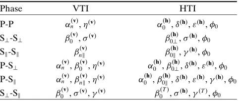
Table 1. Necessary parameters used in the inverse problem to estimate anisotropy.∗

Phase VTI HTI

P-P αn(v),η(v) α₀(h),δ(h),ε(h),φ0

S⊥-S⊥ β (v)

0 ,σ(v) β

(h) 0⊥,σ(h),φ0

Sk-Sk β

(v)

nk β

(h) 0k,γ(h),φ0

P-S⊥ αn(v),β0(v),η(v) α (h) 0 ,β

(h)

0⊥,δ(h),ε(h),φ0

P-Sk αn(v),βn(kv),η(v) α (h) 0 ,β

(h)

0k,δ(h),ε(h),γ(h),φ0

S⊥-Sk β (v)

0 ,σ(v),γ(v) β (T)

0 ,σ(h),γ(T),φ0 ∗_{Note that for laterally homogeneous VTI media the amplitude} of P-Skand S⊥-Skreflections should be zero. Only four parame-ters are needed for S⊥-Skwave propagation in HTI media if the generic Thomsen parametersβ₀(T)andγ(T)_{are used [relations}

(20) and (A-4)].

HTI media.—Unfortunately, in HTI media, phase velocities do depend on azimuth. Therefore, more parameters are needed to accurately describe wave propagation phenomena.

To obtain an idea of the minimum number of parameters required for P-wave data, we need to consider that P-wave NMO velocities in horizontal HTI media show an elliptical variation with azimuth (Tsvankin, 1997b). Hence, three vari-ables are necessary to describe this dependence, namely two NMO velocities and the orientation of a symmetry axis. These parameters could correspond, for instance, to the stack veloc-ityα₀(h)in the isotropy plane, the (short-spread) NMO velocity

αn(h) in the vertical plane containing the symmetry axis, and

the orientation of the symmetry axisφ0. Furthermore, in the

isotropy plane (φ=φ0 ±90◦), moveout is purely hyperbolic.

Hence, P-wave, propagation in this plane is perfectly described by usingα₀(h)only. On the other hand, nonhyperbolic moveout occurs in the other vertical symmetry plane (φ=φ0).

Fortu-nately, since we can construct an equivalent VTI medium, the P-wave moveout in this plane can be accurately computed us-ing solelyα(nh) andη(h). All these quantities are defined in a similar way as their VTI counterparts in relations (33).

Therefore, at least four parameters are needed to calculate P-wave traveltimes in an HTI medium, namelyα₀(h),αn(h),η(h), andφ0. It is naturally possible to recastv(Ph)(pr) [relations (25),

(27), and (29)] in this new form. On the other hand, Tsvankin (1996) showed that the shear-wave velocityβ₀(T)has only a very limited influence on the P-wave velocity. Hence, it is equally well possible to fix the ratioβ₀(h_⊥)/α₀(h)and thereby f(h)_{in these}

equations. This also results in a four-parameter approximation forv(_Ph)(pr) using, say, f(h)=3/4 or 1. In the latter case, we use

again an acoustic approximation which results in ˜

v(_P,ach) (pr)≈α0(h)

×

"

2−6¡

ε(h)−δ(h)¢£w(αh₀)

¤2

2−4ε(h)£

w(αh₀)

¤2

−4¡

ε(h)_−δ(h)¢£

wα(h₀)

¤4 #1/2

, (38)

withw(αh0)given by expression (29). In this form,α (h)

0 equals the

stack velocity in the isotropy plane (φ=φ0±90◦), and the

quan-titiesδ(h)_andε(h)_{are related to the (short-spread) NMO}

veloc-ity and the horizontal velocveloc-ity in the other vertical symmetry plane (φ=φ0), respectively. Furthermore, this choice directly

enables us to invert forα₀(h),δ(h)_{, andε}(h)_{usingP-wave moveout}

information only. This is not possible in the VTI case without any additional information which has to be derived in an in-dependent way (the vertical velocityα₀(v)could for instance be derived from well logs, check shots, or verticle seismic profiles). As a consequence, in HTI media, the vertical P-wave velocity

α₀(h) can be inverted for using surface seismics only. Hence, contrary to VTI media, time-to-depth conversion is possible in HTI media using P-wave traveltime information only.

are needed to describe this variation. On the other hand, the S⊥-velocities within the isotropy plane and along the symme-try axis are identical. Thus, in a first-order approximation, only three parameters are needed. The resulting equations are nearly identical to ˜v(Sv⊥),σ(pr) [equations (35) and (36)]

ex-cept that they are expressed in terms of the equivalent VTI parameters(h)_{. For completeness,}

˜ v(_Sh)

⊥,σ(pr)≈β

(h) 0⊥





−1+2σ(h)£w(_βh)

0⊥

¤2

+©¡1−2σ(h)£w(_βh)

0⊥

¤2¢2

+8σ(h)£w(_βh)

0⊥

¤4ª1/2

4σ(h)£

w_β(h)

0⊥

¤4



 1/2

, (39)

with

w(_βh)

0⊥ =β

(h)

0⊥,i prcos(φ−φ0,i). (40)

The anisotropy parameterσ(h)is defined in a similar way as in expression (37). As a consequence, in a first-order approxima-tion, pure-mode S⊥-moveout is described by three parameters only, namelyβ₀(h_⊥),σ(h)_{, andφ}

0,i.

For P-S⊥waves in HTI media, unfortunately all five parame-ters are needed since the S⊥-velocityβ

(h)

0⊥has a direct influence on the moveout and the ratioβ(₀h_⊥)/α₀(h)cannot be kept constant. Thus, its traveltimes are computed usingα(₀h),β₀(⊥h),δ(h),ε(h), and

φ0,i. Unfortunately, this means that it is impossible to reduce the number of parameters in the inversion process, and recourse has to be taken to the exact equations for the phase velocities

v(ph)(pr) andv(Sh⊥)(pr) [relations (25)–(29)]. As a consequence, no

approximate P-S⊥common conversion points exist.

No reduced-parameter expressions forv_S(h_k)(pr) can be

de-rived either. Table 1 recapitulates the required inversion pa-rameters for all phases.

Parameter estimation.—The new phase velocity functions ˜

v(pv,η)(pr), ˜v

(v)

S⊥,σ(pr), ˜v (h)

P,ac(pr), and ˜v

(h)

S⊥,σ(pr) [relations (34), (35),

(38), and (39)] can be used to calculate approximate traveltime curves of pure-mode data in both HTI and VTI media in a sim-ilar way as before. In addition, they can be used for inversion purposes (paper I). For P-S⊥converted waves and their conver-sion points, reduced-parameter expresconver-sions for the associated phase velocities can only be derived for VTI media. For HTI symmetries, the exact formulas forv(Ph)(pr) andv

(h)

S⊥(pr),

equa-tions (25)–(29), are necessary due to the azimuthal dependence of both the P and S⊥phase velocities.

Nonetheless, the appropriate inversion strategy is straight-forward. First, the seismic data is transformed to the τ-p

domain. Then, the semiellipticalτ(pr) curves are picked for

several reflectors. Next, a so-called layer-stripping approach is applied. That is, the differential intercept times1τi=τi−τi−1

are computed for each layer and horizontal slownesspr [see

equation (2)]. Finally, using a local or global inversion scheme and equation (5) or (6), the observed1τi(pr) curves are fitted

layer by layer to retrieve the anisotropy parameters of each layer, separately. The theoretical phase velocities in terms of the horizontal slowness are identical to those used to calculate approximate traveltimes and conversion points.

In practice, it is easier to pick the curves in the time-offset domain, to calculate the differential moveout which produces

the required slowness (pr=∂t/∂r), and to compute finally

the associatedτ(pr) value using again theτ-ptransform (3).

Moreover, as a quality control, theτ(pr) curves of the picked

traveltime moveout can be overlain on theτ-pgathers of the data. Furthermore, an interactive procedure can be devised in which the picked curves are adapted in and compared with data in both domains.

A general inversion strategy

How can the above-described inversion method be best ap-plied to a seismic data set? First of all, the appropriate inver-sion strategy depends on whether we are dealing with a single 2D line or a complete 3D acquisition geometry. As a quick re-minder, Table 1 shows again the necessary parameters involved for all types of phases and both VTI and HTI symmetries.

2D data.—Naturally the 2D line is the simplest case where we can only consider VTI symmetry due to the lack of azimuthal information. Luckily, if the actual anisotropy symmetry is HTI (e.g., due to vertical cracks), we are still able to replace each vertical plane with an equivalent VTI medium. This follows from the form ofv(Ph)(θ, φ) andv

(h)

S⊥(θ, φ) [relations (22)–(24)].

We are therefore not limited to specific orientations of the seismic line with respect to the actual symmetry axis (e.g., sym-metry planes). Unfortunately, we do make the assumption that out-of-plane effects can be neglected (e.g., conversion points in homogeneous HTI media are not confined to radial planes through the source location). Furthermore, this also amounts to assuming that the medium is laterally homogeneous. Nonethe-less, the inversion strategy is straightforward. Traveltime curves are picked, transformed toτ(pr) curves, and fitted using the appropriate VTI equations.

Note, however, that if the medium actually displays or-thorhombic or lower symmetry, conical points (i.e., point singu-larities) may occur in the phase-velocity sheets of both shear-waves [see, for instance, Crampin (1981) and Crampin and Yedlin (1981)]. The resulting wave behavior cannot be de-scribed assuming a VTI symmetry, and inaccuracies may arise in the inversion results. On the other hand, to the best of our knowledge, conical points have never been observed in seismic field data.

3D data.—If we have a complete 3D data volume, the appro-priate inversion strategy is in principle the same, but becomes practically more involved. On the other hand, a 3D geometry is an absolute prerequisite if the actual anisotropic symmetry is to be established. Due to the increased volume of data, we rec-ommend performing a preliminary analysis of the azimuthal variations of the NMO velocities of the considered horizons first before attacking the complete inverse problem.

arbitrary types of anisotropy. The orientation of the ellipse and the magnitude of its axes can be computed by examining a minimum of three lines through a common midpoint. For HTI symmetry, the fastest NMO velocity corresponds generally to the velocity in the isotropy plane, and conversely the slowest one is parallel to the symmetry axis [assuming thatε(T)_{>0 and}

thusε(h)<0; see equation (20)]. However, in the case of VTI symmetry or isotropy, the ellipse collapses to a perfect circle.

Further a priori knowledge can be acquired by qualitatively looking for nonhyperbolic moveout. Both VTI and isotropic media do not display any azimuthal variation in the NMO ve-locities. However, only VTI symmetry yields nonhyperbolic moveout for P and S⊥-waves if ε(v)6=δ(v) (i.e., nonelliptical anisotropy). Similarly, both HTI and orthorhombic symmetry cause an NMO ellipse. However, in the former case, an isotropy plane without nonhyperbolic moveout must be present, and the nonhyperbolic moveout should be strongest along the second axis of the ellipse. On the other hand, if no isotropy plane can be detected, then we are clearly dealing with a more complicated anisotropy symmetry or strong lateral velocity variations. As a rule of thumb, vertical velocity gradients only cause noticeable nonhyperbolic moveout if the velocity doubles in magnitude within a layer (Hake, 1986; Alkhalifah, 1997).

A distinction between the influence of lateral velocity varia-tions and anisotropy may be difficult to obtain using the present formalism. Nevertheless, indications of lateral inhomogene-ity can be obtained by independently estimating the optimum anisotropy parameters at different locations. In addition, dif-ferent moveout curves for positive and negative offsets at a single common midpoint location also strongly point to lateral changes (Thomsen, 1999).

Once the preliminary NMO velocity analysis has been per-formed and all possible a priori information acquired, an inver-sion strategy identical to that for a single 2D line can be applied. That is, traveltime curves are picked, converted toτ(pr) curves,

and inverted for anisotropy parameters using the appropriate expressions. However, to accurately transform the traveltime picks to theτ-pdomain, slowness must be estimated from the 3D slope of the traveltime surfaces. Picks must be densely dis-tributed, both with distance and azimuth, since otherwise alias-ing may occur. In addition, in order to detect and invert for nonhyperbolic moveout, the ratior/zhas to be larger than 1.5 for all azimuths (Alkhalifah, 1997). This condition must also be met in the 2D case, otherwise deviations from hyperbolic move-out are too small to be measured. Furthermore, this condition must be met regardless whether Taylor-series expansions or

τ-pmethods are used to invert for the anisotropy parameters. NUMERICAL EXAMPLE

As an illustration, we use a strongly anisotropic shale which displays a triplication in the S⊥-moveout curve. Elasticity pa-rameters are taken from Thomsen (1986) and shown in Table 2. Figure 4 displays the slowness and group-velocity surfaces.

Table 2. Elastic parameters of the shale used in the numerical examples (Figures 5–8). All values are taken from Thomsen (1986).

α(₀T) β₀(T) ρ

Generic name (km/s) (km/s) ε(T) _δ(T) _η(T) _σ(T) _γ(T) _(g/cm3₎

Shale (5000) 3.048 1.490 0.255 −0.050 0.339 1.276 0.480 2.420

We consider a three-layer model composed of an uppermost isotropic layer (α=2 km/s,β=1 km/s), an anisotropic shale layer, and again an underlying isotropic layer, (α=4 km/s,

β=2 km/s). Each layer has a thickness of 1 km. The same model was already considered in paper I, but we briefly re-visit it here for illustrative reasons and complete it with the traveltime curves and conversion points of the P-S⊥phase.

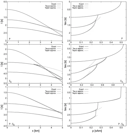
Figure 5 displays the moveout curves. The solid lines are the exact moveout curves and the long-dash lines show the two-parameterτ-p approximations. The P-wave moveout curve is nearly indistinguishable from the exact curve, indicating the high accuracy of approximation (34) for ˜v(Pv,η). The

two-parameter approximation for ˜v(Sv⊥),σ[relations (35) and (36)] for

the S⊥-waves is somewhat less accurate. Nevertheless, it is able to reproduce the cusp. The prediction of P-S⊥moveout is also nearly perfect.

Figure 5 also shows results of the popular Taylor-series ap-proximations (short dashes) (Tsvankin and Thomsen, 1994; Alkhalifah and Tsvankin 1995; Thomsen, 1999). This method produces quite accurate results for the P-wave moveout curves. However, predictions are less accurate than those of the two-parameterτ-pmethod. For S⊥-waves, the Taylor-series method only produces good approximations for short and intermediate offsets (i.e., up to the cusp). Its traveltime predictions for the P-S⊥converted wave are also inferior. Remarkably, the Taylor-series method cannot perfectly describe the P-S⊥traveltimes for reflections of the bottom of the first isotropic layer.

The moveout for Skin VTI media is purely hyperbolic and theτ(pr) curves elliptic. Thus, both methods predict them per-fectly. Similarly, the discrepancy in the predictions for P-Sk con-verted waves solely depends on the accuracy of the P-wave moveout prediction. The errors are therefore comparable to those of the P-wave curves.

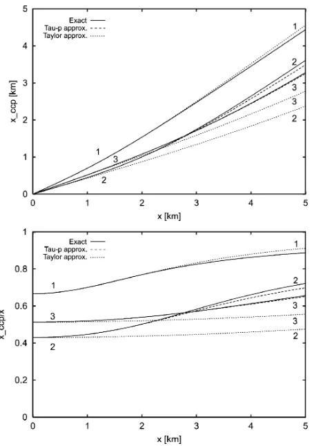
Figure 6 shows the exact (solid line) and approximate (long dashes) conversion points as predicted by theτ-pmethod. The approximations are quite accurate, with maximum errors of 100 m at 5 km offsets. In addition, the conversion point pre-dictions of the Taylor-series method (short dashes) are shown (Thomsen, 1999). Clearly, theτ-pmethod produces much bet-ter results since errors of more than 1 km occur in the predic-tions of the Taylor-series method for the second anisotropic layer.

FIG.5. Traveltimes (left) andτ(pr) curves (right) for the three-layer VTI model for P, S⊥, and P-S⊥converted waves. Note that the Taylor-series method always produces less accurate estimates than theτ-pmethod. Solid line: exact curves; long dashes:τ-p

approximations; short dashes: Taylor-series approximations.

The results in Figures 5 and 6 do not depend on azimuth since a VTI medium is symmetric around the vertical axis. If, on the other hand, the anisotropic shale in Table 2 is tilted by 90◦ (HTI), this is no longer true. Figure 7 displays the exact trav-eltime curves of different seismic phases for reflections of the bottom of the second anisotropic layer. Traveltimes are shown for three different phase azimuths, namely along the symme-try axis (0◦_{), at 45}◦_{, and within the isotropy plane (90}◦_{). For} both P- and P-S⊥-waves, velocities within the isotropy plane are fastest. Conversely, for S⊥-waves at short offsets, S⊥-velocities are slowest within this plane. On the other hand, for longer off-sets, S⊥-velocities for intermediate azimuths (45◦) are fastest.

the results for P-waves are nearly perfect, with errors less than 5 ms at 5 km offset along the symmetry axis. The discrepan-cies for the S⊥-waves are much larger, although predictions are again exact within the isotropy plane. The larger discrep-ancies at the azimuthal phase angle of 45◦ _{are partly due to} the fact that the emergence positions of the exact and approx-imate S⊥-traveltimes are increasingly divergent at larger off-sets. This is due to differences in the directions of the group and phase velocities. Discrepancies are smaller at identical emer-gence positions. For the P-S⊥converted waves, no approximate expressions exist since all five parameters are needed in HTI media (Table 1). Traveltimes for all reflections and conversions from the bottom of the first isotropic layer are naturally exact, and the discrepancies in the predictions of the reflection move-out for the bottom of the third isotropic layer are smaller than those for the second layer.

Figure 7 also shows the Taylor-series approximations for the reflection moveout which exist for pure-mode phases only (Al-Dajani and Tsvankin, 1998). For clarity, these are only displayed for propagation along the 0◦ _{symmetry axis (short} dashes). Within this symmetry plane, theτ-papproximations are clearly more accurate in the far offset, especially in the case of S⊥-S⊥ moveout since the Taylor-series expansions cannot handle kinks or cusps. On the other hand, for short offsets and

FIG.6. Estimations of the common conversion pointsxccpof

P-S⊥converted waves for the three-layer VTI model. Upper part: conversion point distance from the source as a function of emergence offset. Lower part: ratioxccp/x. Numbers corre-spond to layer indices. Solid line: exact curves; long dashes:τ-p

approximations; short dashes: Taylor-series approximations.

an azimuth of 0◦_{, the Taylor-series method is more accurate for} S⊥-S⊥moveout. It should be noted that errors for the Taylor-series expansions are largest within the 0◦_{symmetry plane and} reduce to zero in the isotropy plane (Al-Dajani and Tsvankin, 1998).

Finally, Figure 8 shows a plan view of the conversion points of the P-S⊥and P-Skwaves at the bottom of the second layer. They are displayed in two different bands with declination phase angles of respectively 60◦ _{and 75}◦ _{(measured from the} hori-zontal plane) and 11 phase angle azimuths between 0◦_(x-axis) and 90◦_{(y-axis). The straight lines connect the positions of the} conversion and emergence points on the surface and display therefore the horizontal projections of the upgoing shear rays. For reference, the inner circle of each band links the P-wave midpoints and the outer circle their emergence positions. The exact P-wave midpoints and conversion points for both P-S⊥ and P-Skwaves are coincident for identical radial slownesses and azimuths (Figure 3).

For constant ray (group-velocity) azimuth, the P-wave move-out is confined to radial planes through the source location, whereas the P-S⊥converted waves display out-of-plane effects (except in the two symmetry planes). These out-of-plane con-versions strongly depend on azimuth. On the other hand, the P-Skmoveout hardly deviates from the sagittal plane, and the approximate expressions for the P-Skvelocities are nearly per-fect. No Taylor-series expansions exist for conversion points in HTI media and no comparison could be made.

Figure 8 clearly demonstrates that the estimation of com-mon conversion points in HTI media is a 3D problem (off-set, azimuth, traveltime) even in laterally homogeneous media. Strong variations with both offset and azimuth can occur espe-cially for the P-S⊥-waves. Hence, accurate estimation of all rel-evant anisotropy parameters (Table 1) becomes very important before the problem of sorting into common-conversion-point gathers can be tackled.

DISCUSSION

Our approach of computing traveltimes and conversion points in theτ-pdomain makes it possible to invert for the

underlying anisotropy parameters in both HTI and VTI media (or combinations thereof) using a variety of seismic phases. It is suited for both offshore (streamer only or in combination with ocean-bottom cables) and onshore data (using conventional seismic or even complete nine-component data).

Furthermore, as shown in paper I, for layered, laterally ho-mogeneous regions, a so-called layer-stripping approach is fea-sible. In this approach, traveltime orτ(pr) curves are picked for

different horizons, and the interval1τi curves are computed to isolate the anisotropy in each individual layer. Hence, both effective (average) and local (interval) estimates are obtained. This makes theτ-pmethod a very powerful tool.

Moreover, Diebold (1987) showed that a similar relation between traveltime andτ(pr) curves exists as expression (1)

for 3D isotropic media composed of randomly dipping layers and for more general acquisition geometries other than surface seismic. However, each individual layer has to remain homoge-neous. This remains true for 3D anisotropic structures. Hence, receivers and sources can be positioned at different depths, and

FIG.8. Lateral distribution of conversion points of the base of the HTI layer for P-S⊥and P-Skwaves. Shown are the horizon-tal projections of the upgoing converted rays (straight lines) and the P-wave midpoints and emergence positions (symbols connected by a dot-dash line). The source is placed at the ori-gin. Solid line: exact P-S⊥waves; long dashes: exact P-Skwaves; short dashes: approximate P-Skwaves.

the method can be extended to include for instance verticle-seismic-profile geometries and/or dipping layers. In addition, multiples can be included by making use of their periodicity in theτ-pdomain for flat layers. Unfortunately, for randomly dipping layers, the horizontal slowness is no longer conserved, and the layer-stripping operation becomes more complicated. In addition, care has to be taken if pinch-outs are to be in-cluded. Nonetheless, both exact and approximate traveltimes and conversion points can be computed in randomly dipping HTI and VTI media. Note that the HTI and VTI symmetries are in this case defined with respect to the bottom of each layer. Furthermore, it is possible to predict reflection-point smearing for pure-mode phases (anisotropic dip moveout) and common conversion points in such structures using expression (4).

Finally, expression (5) describing the form of the1τi(pr)

curves remains valid for more general types of anisotropy, including tilted TI media or even lower symmetries like or-thorhombic or monoclinic (with arbitrary orientation of the symmetry axes). Exact formulas for the phase velocities in the crystallographic coordinate system of such media exist (Fryer and Frazer, 1987; Tsvankin, 1996; Tsvankin, 1997a) and can be expressed in terms of Thomsen’s (1986) parameters or gener-alizations thereof (Mensch and Rasolofosaon, 1997; Tsvankin, 1997a; Pˇsenˇc´ık and Gajewski, 1998). Hence, theτ-ptransform is able to calculate exact traveltimes and conversion points in randomly dipping layers with arbitrary type and strength of anisotropy (although a sixth-order polynomial expression with possibly complex roots may have to be solved). In addition, expression (4) can again be used to calculate reflection-point smearing of pure-mode phases in such media and common conversion points. On the other hand, to detect the param-eters most influencing the actual traveltimes and conversion points for different seismic phases and which are appropriate for inversion purposes (Table 1), further analytic treatments are warranted.

CONCLUSIONS

Theτ-papproach is capable of computing exact traveltimes and conversion points for a stratified earth composed of ho-mogeneous layers and arbitrary strength of anisotropy without the need of any ray tracing in the space-time domain. In addi-tion to obtaining exact moveout curves and conversion points, the same method also provides approximate traveltimes and conversion points using reduced-parameter expressions for the phase velocities which are better suited for inversions. These reduced-parameter predictions yield estimates with a nearly always higher accuracy than those provided by the conven-tional Taylor-series expansion. Furthermore, the method has been extended in this paper to handle HTI symmetries for all azimuths and offsets.

Therefore, theτ-papproach can both be used as a forward modeling and inversion tool to assess the anisotropy parame-ters in a particular area. Hence, once these parameparame-ters have been determined, the associated reflection-moveout curves and common conversion points can then be computed using the same approach.

ACKNOWLEDGMENTS