This is a repository copy of Changes in Human Capital and Wage Inequality in Mexico. White Rose Research Online URL for this paper:
http://eprints.whiterose.ac.uk/9947/
Monograph:
Popli, G.K. (2007) Changes in Human Capital and Wage Inequality in Mexico. Working Paper. Department of Economics, University of Sheffield ISSN 1749-8368
Sheffield Economic Research Paper Series 2007001
[email protected] https://eprints.whiterose.ac.uk/
Reuse
Unless indicated otherwise, fulltext items are protected by copyright with all rights reserved. The copyright exception in section 29 of the Copyright, Designs and Patents Act 1988 allows the making of a single copy solely for the purpose of non-commercial research or private study within the limits of fair dealing. The publisher or other rights-holder may allow further reproduction and re-use of this version - refer to the White Rose Research Online record for this item. Where records identify the publisher as the copyright holder, users can verify any specific terms of use on the publisher’s website.
Takedown
If you consider content in White Rose Research Online to be in breach of UK law, please notify us by
Sheffield Economic Research Paper Series
SERP Number: 2007001
Gurleen K. Popli
Changes in Human Capital and Wage Inequality in Mexico
January 2007
Department of Economics University of Sheffield 9 Mappin Street Sheffield S1 4DT United Kingdom
Abstract
Over the last two decades Mexico has witnessed a significant increase in wage inequality, typically attributed to the increase in relative demand for skilled labor. Over this period the educational achievements and their distribution across the labor force have also changed substantially. In this paper we analyze the impact of changes in human capital on wage inequality in Mexico. We focus our analysis on decomposing (1) the level of inequality in any given year and (2) change in inequality over time, into observable (e.g. age, education, occupation, etc.) and unobservable differences across workers. The main findings of this paper are: unobservable factors (within group inequality) account for most of the inequality in any given year. Among the observable factors human capital emerges as the most important variables in explaining the level of, and changes in, inequality.
1. Introduction
Distribution of human capital is one of the most important determinants of the wage
distribution (Card, 1999 and 2001). The impact of human capital can be measured in three
dimensions: changes in average levels, changes in the distribution, and changes in returns.
In Mexico over the last two decades change has been observed in all three dimensions.
Average levels of education have increased, distribution of human capital has become more
equal, and the returns to education have become more unequal. Over this same period
Mexico also witnessed a significant increase in wage inequality.
The literature on rising wage inequality in Mexico has typically attributed it to
increased relative demand for skilled labor leading to increased returns to education (Cragg
and Epelbaum, 1996; Feenstra and Hanson, 1997; Hanson and Harrison, 1999); declining
power of unions (Fairris, 2002); and falling real value of the minimum wage (Cortez, 2001;
Fairris et al, 2006).
An increase in relative demand for skilled labor, leading to increased earnings
inequality is a finding not unique to Mexico.1 What is distinctive about Mexico, however, is
that over this period the educational achievements and their distribution across the labor
force have also changed substantially. That is, the supply of human capital increased as
well. As the supply of skilled labor catches up with the demand, expectation is that
inequality would decrease. In this paper we analyze the impact of changes in human capital
on wage inequality in Mexico, in particular we comment on the impact of the increased
supply of skilled labor on wage inequality – hitherto unexplored for Mexico. Human capital
is acquired in schools and in formal and informal on-the-job training programs, with
in-school acquisition making up an increasingly important component. Here we will focus on
in-school acquisition of skills.
The period covered by this study is 1984 to 2000. We break the two decades into
two distinct periods. The first period, 1984-1994, was marked by structural reforms and
trade and financial liberalization in the economy, rising relative demand for the skilled labor
and rising inequality. The second period, 1994-2000, was one of growth and relative
stability, increasing supply of skilled workers and some evidence of decrease in inequality.
Attempt in this paper is to establish the importance of changing educational endowments and
their distribution in explaining observed changes in wage inequality in Mexico. The analysis
inequality over time, into observable (e.g. age, education, occupation, etc.) and unobservable
differences across workers; the observables are further decomposed into their price
(coefficient) and quantity (endowment) effects.
One other paper which directly looks at the impact of educational endowments on
inequality in Mexico is Legovini et al (2005). This paper is distinct from the Legovini et al
paper in two aspects: (1) our paper looks at a longer horizon. Legovini et al look only at the
first period 1984-1994. The supply of skilled labor takes time to catch up to the increased
demand, by extending the analysis to 2000, unlike Legovini et al, we are able to capture the
impact of increased supply of skilled labor on inequality. (2) The methodology used in this
paper is different than that used by Legovini et al. To answer the levels question we use the
methodology proposed by Fields (2003). The benefit of this approach is, the share
attributable to each explanatory factor, in explaining the level of inequality within a year, is
independent of the measure of inequality used.
The main findings of this paper are as follows. First, the unobservable factors
account for most of the inequality in any given year, giving an indication of a rise in within
group inequality. Second, among the observable factors education and occupation emerge as
important factors in explaining the level of inequality. Third, for changes in inequality over
time, the single most important factor is education. In accordance with the literature we find
that changing returns to skill are important in explaining the rise in inequality. Findings in
this paper suggest that once the supply of skilled labor has had a chance to catch up with the
demand, the quantity effect contributes to the decline in wage inequality.
We begin our analysis by describing the data used in this study and outlining the
changes in average educational endowments of the workforce, their distribution, and returns
to these endowments. The subsequent sections will link the changes in education to wage
inequality.
2. Data
The data used for the analysis is from Encuesta National de Ingresos y Gastos de los
Hogares (ENIGH). These are the national household surveys that began in 1984 and
continued in 1989, 1992, and every two years thereafter. This data is nationally
representative, covers a larger share of population, and has detailed information on the skill
1
levels of the workers.2 The survey employs a ‘stratified sampling’ technique, so we use
sample weights made available by ENIGH in the analysis below.
The sample utilized in this analysis is only of working individuals from the surveyed
households. The earnings variable is real hourly wage (in 1994 pesos), and is computed
from the reported earnings during the month before the survey and reported hours of work
last week. Real wages are obtained by deflating the nominal wages with the consumer price
index, made available by Banco de Mexico. Use of wages is more appropriate in this
analysis since they are more closely related to the market prices for human capital
components. In the estimate of the wage, no fringe benefits, tips, bonuses or commissions
are included. To ensure an accurate measure of the wage, all those who are self-employed3
or working without pay are deleted from the sample. We also exclude from the analysis all
those who hold more than one job.
3. Changes in Human Capital
In this section we describe the changing trends that have been observed in
educational achievements in Mexico over time. Ten education categories are considered: (i)
some primary education; (ii) primary education complete; (iii) junior high incomplete; (iv)
junior high complete; (v) high school incomplete; (vi) high school complete; (vii) some
college; (viii) college complete; and (ix) more than college. The default tenth category is no
education. Both complete and incomplete levels are included as separate categories, as there
is evidence to suggest that there are premiums to completed degree levels.4
Before proceeding a brief comment on the educational structure in Mexico. The
Mexican education system consists of six years of primary education and six years of
secondary education. The secondary education can be broken down into three years of
junior high and three years of high school. Primary education is free and mandatory. In
1992 three years of junior high were also made compulsory. After primary education
students have an option to choose between an academic curriculum (oriented towards
preparation for higher education) and a vocational option (which prepares them for technical
school). For the analysis in this paper we do not distinguish between those who choose a
2
Feenstra and Hanson (1997) and Hanson and Harrison (1999) in their study used macro-survey data of manufacturing plants; Cragg and Epelbaum (1996) in their analysis used micro level data for only 16 urban areas in Mexico.
3
Main reason for excluding the self-employed is the difficulty in distinguishing between the returns to skills and returns to capital for them.
4
technical or an academic option. There might be concerns about not distinguishing between
the two, however the studies conducted on returns to education from different types of
schooling do not find much difference between the two in Mexico (Parker and Pederzin,
2001).
A. Change in average levels and the distribution of education
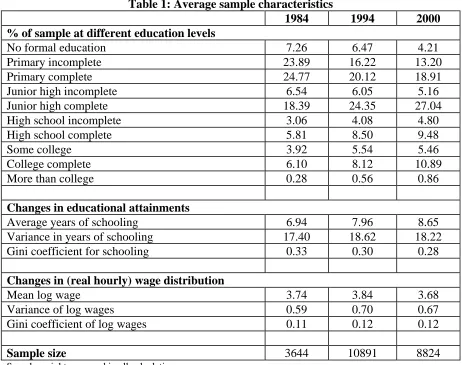
Table 1 gives the proportion of the sample at different education levels in different
years. There has been an overall increase in all education levels above the junior high level
from 1984 to 2000. The share of workers with high school or higher education increased by
10 percentage points – from 16% in 1984 to almost 27% in 2000. The increase in education
levels has been greater for completed degrees. For example, while the proportion of people
with some college education increased by 38% over the period, the proportion of people
completing college and going further increased by almost 79%.
To capture changes in the level and distribution of educational achievements, we
calculate the average years of schooling, variance in years of schooling and the Gini
coefficient for schooling. Data for exact years of schooling are not available from ENIGH.
Until 1994 ENIGH only reported whether or not an individual completed a certain level of
schooling, not the actual years spent in any particular level of schooling. For the completed
levels of schooling we take the years that it would take to complete the level without
repetition. For the incomplete levels of schooling it is assumed that the individual attended
half of the school cycle. These are the standard assumptions made in the literature, in the
absence of data on actual years of schooling (Binder and Woodruff, 2002).5 From 1996
onwards ENIGH started reporting the actual years in school for those with less than 12 years
of schooling. We compare our approximation for 2000 with the actual years; results are
similar. To keep consistency with earlier years we use the approximation for 2000 as well.
Now that we have an approximation to the years of schooling for different
educational levels, we use it to quantify the change in educational achievements over time.
To do so, we calculate three statistics, reported in Table 1:
(1) Average years of Schooling (AYS)
AYS = ∑ ,
= = n
k k k s p y
1
µ
5
where, n is the number of educational groups (for this study n = 10), be the years of
schooling at different education levels, is the proportion of people in the k k
y
k
p th educational
category (for this study proportions for the different years are given in Table 1).
(2) Variance in Schooling (VS)
VS = ∑ ,
= −
= n
k k k s
s p y
1
2 2
)
( µ
σ
(3) Gini Coefficient for Schooling (GINIS)
∑ ∑ =
−
= −
⎟⎟ ⎠ ⎞ ⎜⎜ ⎝ ⎛
= n
k k
l k k l l
s
s p y y p
GINI
2 1
1
1
µ .
The average years of schooling have increased in Mexico over the period 1984 to
2000.6 The variance in years of schooling has increased slightly, but that is not surprising as
variance captures absolute dispersion and increases with increasing mean. To look at
relative dispersion we look at the Gini coefficient, according to which the inequality in the
distribution of education has decreased over time.
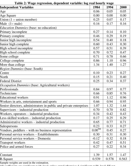
B. Change in the returns to education
To capture changes in the returns to education we run a weighted least square
log-wage regression, where the dependent variable is the log of real hourly log-wages and the
explanatory variables are: age, age-squared, nine education dummies (‘no formal education’
is the base), gender, union status, three regional dummies and fifteen occupation dummies.
Regression results are reported in Table 2.
Looking at the coefficients of the education dummies, the gap between the returns to
lower and higher education has increased over time, with most of the increased gap coming
from a decline in the returns to lower skill groups. Rising relative rates of return to
educational attainments may reflect the importance of demand-side factors related to
liberalization and foreign investment or they may reflect changing institutional factors such
as the declining real value of the minimum wage, which other results (Cortez, 2001; Fairris,
2002; Fairris et al, 2006) suggest have had a significantly greater impact on low-skill
workers relative to high-skill workers.
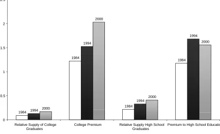
To summarize the information on the education dummies, in Figure 1 we plot the
‘college premium’ and the ‘relative supply of college graduates’. The ‘college premium’ is
school degree’ in the wage regression; and the ‘relative supply of college graduates’ is
defined as the ratio of college equivalents (those with at least college + 0.5 × those with
some college) to non-college equivalents (those with high school or less + 0.5 × those with
some college).7 Even though the relative supply of college graduates has been increasing
over the period under study, the college premiums have also been increasing. This indicates
that the demand for skilled workers (as captured by college or more education) has been
increasing faster than the supply of skilled workers.
Labor in Mexico is less skilled than in developed countries like the U.S., so perhaps a
college degree is too high a threshold in designating the ‘highly skilled’. In Figure 1 we also
show the ‘high school premium’ and ‘relative supply of high school graduates’. The
premium to high school education is the ratio of the coefficient on ‘high school degree’ to
the coefficient on ‘junior high degree’ in the wage regression. As before, the relative supply
of high school graduates is the ratio of high school equivalents (those with at least high
school degree + 0.5 × those with high school incomplete) to non-high school equivalents
(those with junior high or less + 0.5 × those with some high school). The story here is
slightly different. Both supply of and premium to high school graduates increased till 1994,
indicating greater increase in demand than supply, however after that while the supply has
continued to increase, the premium has declined. This could indicate supply catching up
with demand.
4. Wage Inequality
How are the above changes in the levels, distribution and returns to skill related to
wage inequality? We begin this analysis by briefly outlining recent changes in the
distribution of wages.
A. Changes in the wage distribution
In Table 1 we report the mean log wage, variance of log wages and the GINI
coefficient for the log wage. The mean log wage increased until 1994 and decreased
thereafter, such that any gains made in real wages up to 1994 were completed eroded by
2000. This decline in real wages is by and large a result of the 1995 peso crisis, after which
though the real wages recovered a little they never reached the highs of pre-crisis period.
6
This is consistent with the findings of Duryea and Szekely (1998) and Legovini et al (2005).
7
Period of structural reforms and trade and financial liberalization (1984-1994) in Mexico is
associated with the increase in inequality, after which the inequality started to decline or at
least stabilized (depending on the measure of inequality used).
B. Accounting for within-year inequality
To account for the different factors contributing to inequality we use the procedure
proposed by Gary Fields (2003). Consider the wage regression,
(4) = ∑+ ,
=
2
1
ln
J
j jt jit it a Z w
where wit is the wage of the ith individual in the tth time period,
] 1 ...
[ t 1t 2t Jt
t
a = α β β β and Zit =[1 X1it X2it ... XJit εit] are vectors of
coefficients and the explanatory variables (including the residual term), respectively. For the
wage regression of the form given in equation (4) and using the variance of log wages as a
measure of inequality, Fields shows that the share of the variance of log wages that is
attributable to the jth explanatory variable can be written as:
(5) ) (ln ) ln , .( ) ( w w Z Cor Z a
sj j j j
σ σ
= ,
where, σ(.) is the standard deviation of the variable and is the correlation
between the explanatory variable and lnw. is also called the ‘relative factor inequality
weight’, such that , and of the regression in (4). The advantage of
using Field’s method to estimate the relative factor inequality weights is that it is not
sensitive to the measure of inequality used.
) ln ,
.(Z w
Cor j j s % 100 2 1 = ∑+ = J j j s 2 1 1 R s J j j = ∑+ = j
s can be calculated for every explanatory variable in the wage regression. We have
nine dichotomous variables for education in the model, and a measure is calculated for
each of them. To estimate the total share of education in explaining wage inequality, the
’s for the entire set of education dummies are summed together. Similarly, we can
estimate the total relative factor inequality weight for the other categorical variables, like
region and occupation, in the wage equation. For age we sum the weights for age and age
squared.
j
s
j
s
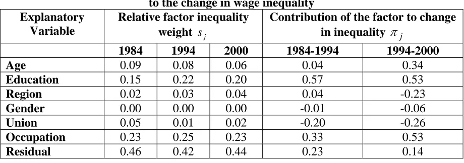
The relative factor weights for the different explanatory variables for 1984, 1994 and
mean wages, not all of them have equal weight in explaining the level of inequality. For all
three years the unobservable factors (residuals) are most important in explaining the level of
inequality. After the residuals the most important variable explaining inequality is
occupation followed by education; however, if we use age and education together as human
capital variables then they together account for a bigger share of inequality. Gender is not
important, the importance of union has decreased over time, while the effect of region has
increased.8
C. Decomposing the change in across-year inequality
The Change in inequality over time can be written as:
(6) − =∑ − ,
j j j
w s
w s
w
w ) (ln ) [ (ln ) (ln )]
(ln 2 2 1 2 2 2 1 2 1
2 σ σ σ
σ
where 1 and 2 represent two time periods. The contribution of the jth factor to the change in
inequality can in turn be written as:
(7) ) (ln ) (ln ) (ln ) (ln 1 2 2 2 1 2 1 2 2 2 w w w s w
sj j
j σ σ σ σ π − − = ,
such that ∑ =100% j j
π . We calculated the contribution of the different factors to changing
inequality over the 1984-1994 and 1994-2000 periods, the results are reported in Table 3.
Larger πj indicates a larger contribution of the jth factor to change in inequality, which in
turn could indicate the following: jth factor contributes to the increase (decrease) in
inequality due to (i) a larger increase (decrease) in the regression coefficient of the jth factor,
and/or (ii) a large increase (decrease) in the variation of the jth factor.
For both the period of rising and decreasing inequality, education has the largest
contribution to the change in inequality. Second most important factor after education is
occupation, in fact the importance of occupation in explaining the change in inequality has
increased over time. While for the period of rising inequality gender and unions had an
equalizing impact, for the period of falling inequality the two factors were working in the
direction of raising inequality. The importance of age and region in explaining the changes
in inequality increased over the two periods. While changes in age accounted for only a
small part of increasing inequality, it was a big factor in explaining the fall in inequality.
8
Regional variations continue to exert an upward pressure on inequality, more so in the
second period.9
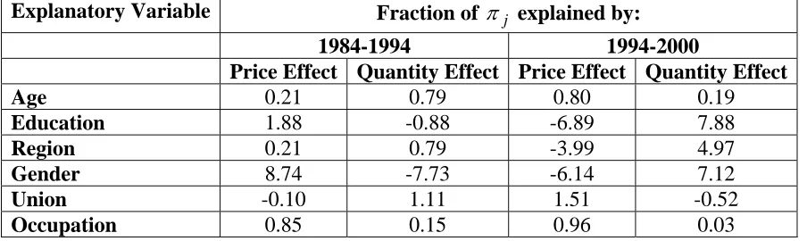
D. Price and quantity effects
If education is important in explaining the change in inequality over time, it is of
interest to know – whether it is the changing returns to education (the price effect) or the
changing levels of education (quantity effect) that is important. The contribution of any
factor to the change in inequality can be decomposed into its price and quantity effects as
argued by Yun (2002) and Juhn, Murphy and Pierce (1993). To do this we define a
counterfactual regression, (subscript c denotes counterfactual), adding and
subtracting this to equation (6) we get:
∑
= +
=
2
1 1 2
ln
J
j j ji ic a Z w (8) , )] (ln ) ln , .( ) (ln ) ln , .( [ )] (ln ) ln , .( ) (ln ) ln , .( [ ) (ln ) (ln ) (ln ) (ln ) (ln ) (ln 1 1 1 1 1 2 2 1 2 2 1 2 2 2 2 2 1 2 2 2 2 2 1 2 2 2
∑
∑
∑
∑
+ = − + − = − + − = − j j j j j j j j c c j j j c c j j j j j j j c c QE PE w w Z cor a w w Z cor a w w Z cor a w w Z cor a w w w w w w σ σ σ σ σ σ σ σ σ σ σ σ σ σwhere the first summation is the price effect, with PEj being the price effect of the jth
variable, and the second summation is the quantity effect, with being the quantity effect
of the j
j
QE
th
variable. Using equations (6) and (7), we can decompose the contribution of the jth
factor to the change in inequality as j j
j j j q w w QE PE + = − + = ρ σ σ π ) (ln )
(ln 2 2 1
2 , giving us
(9) j j j j q π π ρ + = 1 ,
where the first part of equation (9) is the fraction of the contribution of the jth factor to the
change in inequality due to its price effect and the second part is due to the quantity effect.
To estimate the total effect of a categorical variable on the change in inequality we
propose the following: let πc be the share of the categorical variable explaining the change
in inequality. Define , where k is the total number of dummy’s representing the
categorical variable (in this paper for education k = 9, for occupation k = 15, and for region k ∑ = = k l l c 1 π π 9
= 3) and πl is estimated using equation (7). πc can be decomposed into price and quantity
effect as =∑ =∑ +
l l l l l
c π (ρ q )
π , from which we get:
(10)
c l
c
l q
π π
ρ +∑
∑ =
1 .
The fraction of the change in πc attributable to the price effect is given by the first term of
equation (10) and the fraction attributable to the quantity effect is given by the second term
of the equation. Using equations (8), (9) and (10) we decompose the contribution of the
factor to the change in inequality into its price and quantity effect. The results are reported
in Table 4.
Increasing returns to education (i.e. the price effect) contributed to the rise in
inequality and increasing endowments of education (i.e. the quantity effect) as expected
contributed to a decrease in inequality, over both the periods. For the period of rising
inequality, the price effect dominated, indicating that demand for skilled workers increased
faster than supply.10 Subsequently as the supply of skilled labor caught up to the demand the
quantity effect dominates the price effect, thus education overall contributes to a decrease in
inequality in the second period.
The second most important component of rising wage inequality is occupation, which
may incorporate human capital attainment on the job in the form of job training. It is the
changing returns to occupation and not the changing occupational mix that appears to
account for both the increase and decrease in inequality.
6. Conclusion
In this paper we focused on the impact of changing human capital skills on wage
inequality in Mexico. While a number of papers have commented on the impact of changing
relative demand for skilled labor on wage inequality in Mexico, not much has been said
about the impact of the changing supply of skilled labor. Our findings suggest that education
plays an important role in both the dispersion of wages among Mexican workers and in
changes in this dispersion over time. The results not only document the degree of
importance of education in wage dispersion in Mexico, they also reveal that both the
changing returns to education and the changing educational attainments are important factors
in the increasing, and then decreasing, wage inequality over the past two decades. Over the
10
period of trade liberalization and structural reforms in the country the demand for skilled
labor increased, which lead to an increase in returns to education and increases in wage
inequality. However as the supplies of skilled labor caught up to the demand, inequality
References
Autor, David, Lawrence Katz and Alan Krueger. 1998. “Computing Inequality: Have Computers Changed the Labor Market,” Quarterly Journal of Economics, vol. 113, pp. 1169-213.
Behram, Jere R. and Anil B. Deolalikar. 1991. “School Repetition, Dropouts, and the Rates of Return to Schooling: The Case of Indonesia,” Oxford Bulletin of Economics and
Statistics, vol. 53, no. 4, pp. 467-480.
Binder, Melissa and Christopher Woodruff. 2002. “Inequality and Intergenerational Mobility of Schooling: The Case of Mexico,” Economic Development and Cultural
Change, vol. 50, pp. 249-267.
Card, David. 1999. “The Casual Effect of Education on Earnings,” in Orley Ashenfelter and David Card, (eds), Handbook of Labor Economics, (North Holland), vol. 3, pp. 1801-1863.
Card, David. 2001. “Estimating the Return to Schooling: Progress on some persistent Econometric Problems,” Econometrica, vol. 69, no. 5, pp. 1127-1160.
Cortez, W. W. 2001. “What is Behind Increasing Wage Inequality in Mexico,” World
Development 29 (11): 1905-1922.
Cragg, Michael and Mario Epelbaum. 1996. “Why has Wage Dispersion grown in Mexico? Is it the Incidence of Reforms or the Growing Demand for Skill?” Journal of
Development Economics, vol. 51, pp. 99-116.
Duryea, Suzanne and Miguel Szekely. 1998. “Labor markets in Latin America: A Supply-Side Story,” Working Paper 374, Inter-American Development Bank, Office of the Chief Economist.
ENIGH Encuesta National de Ingresos y Gastos de los Hogares, INEGI, for various years. Fairris, David. 2002. “Unions and Wage Inequality in Mexico,” Industrial and Labor
Relations Review, vol. 56, no. 3, pp. 481-97.
Fairris, David, Gurleen Popli, and Eduardo Zepeda. 2006. “Minimum Wages and the Wage Structure in Mexico,” Review of Social Economy (forthcoming).
Feenstra, Robert C., and Gordon H. Hanson. 1997. “Foreign Direct Investment and Relative Wages: Evidence from Mexico’s Maquiladoras,” Journal of International
Economics, vol. 42, pp. 371-393.
Fields, Gary. 2003. “Accounting for Income Inequality and its Change: A New Method, with Application to the Distribution of Earnings in the United States,” Research in Labor
Economics.
Hanson, G.H. 2003. “What has happened to Wages in Mexico since NAFTA? Implication for Hemispheric Free Trade,” Working Paper no. 9563, NBER.
Hanson, Gordon H., and Ann Harrison. 1999. “Trade Liberalization and Wage Inequality in Mexico,” Industrial and Labor Relations Review, vol. 52, no. 2, pp. 271-288.
Juhn, Chinhui, Kevin Murphy and Brooks Pierce. 1993. “Wage Inequality and the Rise in Returns to Skill,” Journal of Political Economy, vol. 101, pp.410-42.
Katz, Lawrence and David Autor. 1999. “Changes in the Structure and Earnings Inequality,” in Orley Ashenfelter and David Card, (eds), Handbook of Labor Economics, (North Holland), vol. 3, pp. 1463-1555.
Legovini, A., C. Bouillon and N. Lustig. 2005. "Can Education Explain Changes in Income Inequality in Mexico?" in F. Bourguignon, F.H.G. Ferreira, and N. Lustig, (eds), The
Microeconomics of Income Distribution Dynamics: in East Asia and Latin America,
(A co-publication of World Bank and Oxford University Press), pp. 275-312.
Parker, Susan W. and Carla Pederzini. 2001. “Gender Differences in Education in Mexico,” in Elizabeth Katz and Maria Correia, (eds.), The Economics of Gender in Mexico, (The World Bank Publication), pp. 9-45.
Table 1: Average sample characteristics
1984 1994 2000 % of sample at different education levels
No formal education 7.26 6.47 4.21
Primary incomplete 23.89 16.22 13.20
Primary complete 24.77 20.12 18.91
Junior high incomplete 6.54 6.05 5.16
Junior high complete 18.39 24.35 27.04
High school incomplete 3.06 4.08 4.80
High school complete 5.81 8.50 9.48
Some college 3.92 5.54 5.46
College complete 6.10 8.12 10.89
More than college 0.28 0.56 0.86
Changes in educational attainments
Average years of schooling 6.94 7.96 8.65
Variance in years of schooling 17.40 18.62 18.22
Gini coefficient for schooling 0.33 0.30 0.28
Changes in (real hourly) wage distribution
Mean log wage 3.74 3.84 3.68
Variance of log wages 0.59 0.70 0.67
Gini coefficient of log wages 0.11 0.12 0.12
Sample size 3644 10891 8824
Sample weights are used in all calculations.
Since we are using sample weights throughout, the standard formula for calculating the Gini coefficient cannot be used. Instead we use the procedure for calculating the Gini coefficient for weighted samples as given by Lerman and Yitzhaki (1989).
Table 2: Wage regression, dependent variable: log real hourly wage
Independent Variables 1984 1994 2000
Age 0.06 0.05 0.05
Age Square 0.00 0.00 0.00
Union (1 = union member) 0.25 0.07 0.17
Male (1= male) 0.16 0.17 0.16
Education Dummies (base: no education)
Primary incomplete 0.27 0.14 0.10
Primary complete 0.46 0.29 0.19
Junior high incomplete 0.54 0.40 0.18
Junior high complete 0.60 0.43 0.30
High school incomplete 0.57 0.51 0.39
High school complete 0.70 0.72 0.47
Some college 0.71 0.78 0.66
College complete 0.86 1.10 0.96
More than college 1.34 1.40 1.27
Region Dummies (base: South)
Centre 0.10 0.23 0.27
North 0.15 0.21 0.40
Federal District 0.25 0.34 0.37
Occupation Dummies (base: Agricultural workers)
Professionals 0.84 0.97 0.77
Technicians 0.66 0.85 0.76
Educational workers 0.91 1.12 0.96
Workers in arts, entertainment and sports 0.66 0.94 0.95
Senior directors, administrators in public and private enterprises 1.07 1.32 1.44
Supervisors – industrial production 0.70 0.70 0.82
Workers, operators – industrial production 0.34 0.42 0.43
Less-skilled workers – industrial production 0.17 0.25 0.29
Administrative workers – industrial production 0.65 0.77 0.71
Salespersons 0.23 0.33 0.27
Vendors, peddlers – with no business representation 0.00NS 0.45 0.27
Personal service workers – Establishments 0.30 0.31 0.30
Personal service workers – Domestic -0.12* 0.32 0.18
Transport workers 0.42 0.47 0.51
Police and armed forces 0.27 0.22 0.34
Constant 1.39 1.57 1.47
R-Square 0.539 0.578 0.563
Sample weights are used in the estimation.
All coefficients are significant at 1% level, unless stated otherwise: * significant at 5% level; NS not significant.
Region Dummies Center: Aquascalientes, Colima, Jalisco, Michoacan, Guanajuato, Queretaro, Morelos,
Tlaxcala, Puebla, Hidalgo, Mexico. North: Baja California, Baja California Sur, Sinaloa, Sonora, Nayarit, Nuevo Leon, Tamaulipas, Chihuahua, Durango, Coahuila, San Luis Potosi, Zacatecas. South (base): Guerrero, Oaxaca, Chiapas, Veracruz, Tabasco, Yucatan, Campeche, Quintana Roo.
Table 3: Contribution of each explanatory variable to the level of wage inequality and to the change in wage inequality
Explanatory Variable
Relative factor inequality weight sj
Contribution of the factor to change in inequality πj
1984 1994 2000 1984-1994 1994-2000
Age 0.09 0.08 0.06 0.04 0.34
Education 0.15 0.22 0.20 0.57 0.53
Region 0.02 0.03 0.04 0.04 -0.23
Gender 0.00 0.00 0.00 -0.01 -0.06
Union 0.05 0.01 0.02 -0.20 -0.26
Occupation 0.23 0.25 0.23 0.33 0.53
Residual 0.46 0.42 0.44 0.23 0.14
j
s is calculated based on equation (5) in the paper; πj is calculated based on equation (6) in the paper.
Table 4: Decomposing the contribution of each explanatory variable to the change in wage inequality
Explanatory Variable Fraction of πj explained by:
1984-1994 1994-2000
Price Effect Quantity Effect Price Effect Quantity Effect
Age 0.21 0.79 0.80 0.19
Education 1.88 -0.88 -6.89 7.88
Region 0.21 0.79 -3.99 4.97
Gender 8.74 -7.73 -6.14 7.12
Union -0.10 1.11 1.51 -0.52
Occupation 0.85 0.15 0.96 0.03
j
π is calculated based on equation (5) in the paper, decomposition is done using equations (8), (9) and (10).
Figure (1) Relative supply and returns to skilled labor
2.5
2000 2
1994
2000 1994
1.5
1984
1984
1
0.5 2000
1994 1984 2000
1994 1984
0
Relative Supply of College College Premium Relative Supply High School Premium to High School Education
Graduates Graduates
College premium is the ratio of the coefficient on ‘college degree’ relative to the coefficient on ‘high school degree’ in the wage regression.
Relative supply of college graduates is the ratio of college equivalents (those with at least college + 0.5 × those with some college) to non-college equivalents (those with high school or less + 0.5 × those with some college). High school premium is the ratio of the coefficient on ‘high school degree’ to the coefficient on ‘junior high degree’ in the wage regression.
Relative supply of high school graduates is the ratio of high school equivalents (those with at least high school degree + 0.5 those with high school incomplete) to non-high school equivalents (those with junior high or less + 0.5 × those with some high school).
×
[image:21.595.82.514.113.377.2]