Robot programming by demonstration through system identification

This is a repository copy of

Robot programming by demonstration through system

identification

.

White Rose Research Online URL for this paper:

http://eprints.whiterose.ac.uk/74607/

Monograph:

Nehmzow, U., Akanyeti, O., Weinrich, C. et al. (2 more authors) (2007) Robot

programming by demonstration through system identification. Research Report. ACSE

Research Report no. 948 . Automatic Control and Systems Engineering, University of

Sheffield

[email protected] https://eprints.whiterose.ac.uk/ Reuse

Unless indicated otherwise, fulltext items are protected by copyright with all rights reserved. The copyright exception in section 29 of the Copyright, Designs and Patents Act 1988 allows the making of a single copy solely for the purpose of non-commercial research or private study within the limits of fair dealing. The publisher or other rights-holder may allow further reproduction and re-use of this version - refer to the White Rose Research Online record for this item. Where records identify the publisher as the copyright holder, users can verify any specific terms of use on the publisher’s website.

Takedown

If you consider content in White Rose Research Online to be in breach of UK law, please notify us by

Robot Programming by Demonstration Through System

Identification

U Nehmzow

, O. Akanyeti

, C Weinrich

, T Kyriacou

, S A Billings

#Dept Computer Science, University of Essex

Department of Automatic Control and Systems Engineering

The University of Sheffield, Sheffield, S1 3JD, UK

Research Report No. 948

Robot Programming by Demonstration through System Identification

U. Nehmzow

, O. Akanyeti

, Christoph Weinrich

, Theocharis Kyriacou

and S.A. Billings

Abstract— Increasingly, personalised robots — robots espe-cially designed and programmed for an individual’s needs and preferences — are being used to support humans in their daily lives, most notably in the area of service robotics. Arguably, the closer the robot is programmed to the individual’s needs, the more useful it is, and we believe that giving people the opportunity to program their own robots, rather than programming robots for them, will push robotics research one step further in the personalised robotics field.

However, traditional robot programming techniques require specialised technical skills from different disciplines and it is not reasonable to expect end-users to have these skills. In this paper, we therefore present a new method of obtaining robot control code — programming by demonstration through system iden-tification — which algorithmically and automatically transfers human behaviours into robot control code, using transparent, analysable mathematical functions. Besides providing a simple means of generating perception-action mappings, they have the additional advantage that can also be used to form hypotheses and theoretical analysis of robot behaviour.

We demonstrate the viability of this approach by teaching a Scitos G5 mobile robot to achieve wall following and corridor passing behaviours.

I. INTRODUCTION

Interest in the field of programming mobile robots by demonstration — teaching the robot to achieve a certain behaviour by simply demonstrating it — has been growing steadily in the last few years. Significant advantages of this approach are:

• Efficiency in generating robot controllers:

Tradi-tional robot programming techniques are costly, time-consuming and error prone [Iglesias et al., 2005].

• Little or no need for programming skills: The

program-mer does not have to have any specialised programming skills, end-users can “program” their robots individually according to their own preferences and needs by demon-stration.

• Implicit communication: No explicit communication is

needed between the robot and the programmer. The programmer communicates with the robot through the environment by demonstrating the desired behaviour. Many researchers have shown the viability of this approach by teaching robots different tasks such as for example maze navigation [Demiris and Hayes, 1996], [Hayes and Demiris, 1994] and arm movement [Schaal, 1997].

In this paper, we present a method to transfer human behaviours to robot control code algorithmically and au-tomatically, using system identification techniques such as

1_{Department of Computer Science, University of Essex, UK}

2_{Department of Automatic Control and Systems Engineering, University}

of Sheffield, UK.

ARMAX (Auto-Regressive Moving Average models with eXogenous inputs) [Eykhoff, 1974] and NARMAX (Non-linear ARMAX) [Billings and Chen, 1998]. These system identification techniques produce linear or nonlinear poly-nomial functions that model the relationship between user-defined input and output, both pertaining to the robot’s behaviour.

The representation of the task as a transparent, analysable model furthermore enables us to investigate the various factors that affect robot behaviour for the task at hand. For instance, we can identify input-output relationships such as the sensitivity of a robot’s behaviour to particular sensors [Roberto Iglesias and Billings, 2005], or make predictions of behaviour when a particular input is presented to the robot [Akanyeti et al., 2007] — these aspects are relevant to safety analyses.

II. METHODOLOGY AND EXPERIMENTAL SETUP

Before we discuss the experimental setup and results obtained, we briefly explain the Narmax system identification method, which was used throughout our experiments.

A. The NARMAX Modelling Methodology

The NARMAX modelling approach is a parameter estima-tion methodology for identifying both the important model terms and the parameters of unknown nonlinear dynamic systems. For multiple input, single output noiseless systems this model takes the form:

y(n) = f(u1(n),u1(n−1),u1(n−2),· · ·,u1(n−Nu),

u1(n)2,u1(n−1)2_,u 1(n−2)2_,

· · ·,u1(n−Nu)2_,

· · ·,

u1(n)l,u1(n−1)l_,u

1(n−2)l_,

· · ·,u1(n−Nu)l_,

u2(n),u2(n−1),u2(n−2),· · ·,u2(n−Nu),

u2(n)2,u2(n−1)2,u2(n−2)2,· · ·,u2(n−Nu)2_,

· · ·,

u2(n)l,u2(n−1)l,u2(n−2)l,· · ·,u2(n−Nu)l, · · ·,

· · ·,

ud(n),ud(n−1),ud(n−2),· · ·,ud(n−Nu), ud(n)2,ud(n−1)2_,u

d(n−2)2_,

· · ·,ud(n−Nu)2,

· · ·,

ud(n)l,ud(n−1)l_,u d(n−2)l_,

· · ·,ud(n−Nu)l,

y(n₋1),y(n₋2),· · ·,y(n−Ny),

y(n₋1)2_,y(n

−2)2,· · ·,y(n−Ny)2, · · ·,

y(n₋1)l_,y(n

−2)l,· · ·,y(n−Ny)l)

of the input vector andlis the degree of the polynomial. f()

is a non-linear function and here taken to be a polynomial multi-resolution expansion of its arguments. Expansions such as multi-resolution wavelets or Bernstein coefficients can be used as an alternative to the polynomial expansions considered in this study.

The first step towards modelling a particular system using a NARMAX model structure is to select appropriate inputs

u₍n) and the output y(n). The general rule in choosing suitable inputs and outputs is that there must be a causal re-lationship between the input signals and the output response. After the choice of suitable inputs and outputs, the NAR-MAX methodology breaks the modelling problem into the following steps: i) polynomial model structure detection, ii) model parameter estimation and iii)model validation. The last two steps are performed iteratively (until the model estimation error is minimised) using two sets of collected data: (a) the estimation and (b) the validation data set. Usually a single set that is collected in one long session is split in half and used for this purpose.

The model estimation methodology described above forms an estimation toolkit that allows the user to build a con-cise mathematical description of the input-output system under investigation. These procedures are now well estab-lished and have been used in many modelling domains [Billings and Chen, 1998].

A more detailed discussion of how structure detection, parameter estimation and model validation are done is presented in [Korenberg et al., 1988], [Billings and Voon, 1986].

B. Experimental Setup

The experiments described in this paper were conducted in the 100 square meter circular robotics arena of the University of Essex. The arena is equipped with a Vicon motion tracking system which can deliver position data (x,y and z) for the full range of targets using reflective markers and high speed, high resolution cameras. The tracking system is capable of sampling the motion upto 100Hz within a 10mm range accuracy.

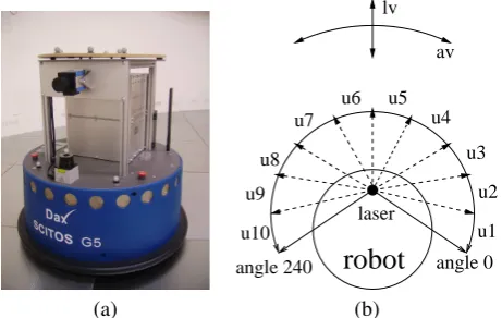
We used a Scitos G5 mobile robot called DAX(figure 1). The robot is equipped with a ring of 24 sonar and 24 infra-red sensors, both uniformly distributed. A Hokuyo laser range finder is also present on the front part of the robot. This range sensor has a wide angular range (240 degree) with a radial resolution of 0.36 degree and distance resolution of less than 1cm. The robot also incorporates a colour video camera with 640x480 pixels resolution which can deliver colour images upto 60Hz.

robot

angle 240 angle 0 laser u4 u3 u2 u1 u5 u6 u7 u8 u10 u9 av lv (a) (b)

Fig. 1. DAX (a). DAX has two degrees of freedom (translational and rotational) and equipped with the laser range finder. The range finder has a wide angular range (240 degree) with a radial resolution of 0.36 degree and distance resolution of less than 1 (cm). During experiments, in order to decrease the dimensionality of the input space to Narmax model, we coarse coded the laser readings into 10 sectors (u1tou10) by averaging 62

readings for each 24 degree intervals (b).

C. Programming by Demonstration

While teaching a particular task to a robot, it is difficult to establish a proper information flow from the programmer to the robot, because humans and robots have different sensor modalities — we simply perceive the world differently to robots. We have therefore chosen the mobile robot’s trajectory of the desired behaviour as the most suitable communication channel between the human and the robot in question. We therefore take the trajectory of a human as a reference, and translate it algorithmically and automatically into robot control code.

Our approach has three stages: i) first extracting the tra-jectory of the desired behaviour by observing the human, ii) making the robot follow the human trajectory blindly to log the robot’s own perception perceived along that trajectory, and finally iii) linking the robot’s perception to the desired behaviour to obtain a generalised, sensor-based model.

Human Demonstration: First, the human user demon-strates the desired behaviour. In this work, we confined our experiments to two-dimensional navigation problems (two degrees of freedom, translational and rotational speed, see figure 1). During this demonstration, we log the x and y

position of the human by using a motion tracking system with a sampling rate of 50Hz.

Ts=

Ns

fc∗fs

(1)

whereNsis the number of samples logged, fcis the cut off frequency of low pass filter and fs is the sampling rate of the motion tracking system.

The translational and rotational velocitieslvandavresp. of the demonstrator are determined by taking into account of the consecutivex,ysamples along the trajectory (equation 3).

lv(n) =distance(n) timedi f f(n)

(2)

av(n) = theta(n) timedi f f(n)

where

distance(n) =p(xn+1−xn)2+ (yn+1−yn)2, (3)

theta(n) =arctan(yn+1−yn) (xn+1−xn)

), (4)

and

timedi f f(n) =tn+1−tn. (5)

Obtaining the sensor-free time series: At this point we have extracted the translational and rotational velocities of the human demonstrator along his trajectory. We now need to transfer these velocities to the robot while taking the dynamics of the robot into consideration. Therefore two sensor free polynomial models are obtained: i) expressing rotational velocity commands as a function of time and past rotational velocity commands and ii.) expressing linear velocity commands as a function of time and past linear velocity commands.

lv(t) av controller

lv controller

av(t) [av(t−1), av(t−2), ..., av(t−N)]

time

[lv(t−1), lv(t−2), ..., lv(t−N)] time

sensor free

sensor free

Fig. 2. The sensor-free polynomial models. Sensor-free models don’t use any perceptual information, they follow the trajectory of human blindly. Positivelvand negativelvindicate that robot goes forward and backward respectively. Positiveavand negativeavindicate that robot turns left and right respectively.

Obtaining the sensor-based controllers: Having ob-tained the sensor-free models, we use them to drive the robot along the trajectory of the human, blindly, so to speak. During this run the sensor perceptions of the robot are logged every 100ms, together with the robot’s translational and rotational velocities.

Using this based data, we then obtain two sensor-based control models, one for translational velocity and one for rotational velocity (see figure 3).

(sonar, laser, etc) sensor readings

(sonar, laser, etc)

sensor readings _lv(t)

av controller

lv controller

av(t) sensor based

sensor based

Fig. 3. Sensor based models. Sensor based models are the mathematical descriptions that define the relationship between the perception and action of the robot. Because they take sensor information into account, they are capably of controlling the robot in a wider range of situations, and to deal with noise and variation.

III. EXPERIMENTS AND RESULTS

A. Left Wall Following

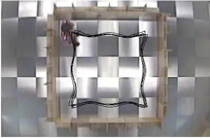
In our first experiment, we demonstrated to the robot how to follow left-hand walls. The demonstrator walked inside a square environment of 9m2 in clockwise direction for approximately two minutes (see figure 4). During this time, the position of human was logged every 20ms.

Fig. 4. The desired convex wall following behaviour demonstrated by the human in a square environment. When we look at the trajectory, we see that there is a constant oscillation in the motion, which originates from the swinging motion of the demonstrator perpendicular to heading direction. This is a general characteristic of two legged locomotion, and was subsequently removed from the data by low pass filtering.

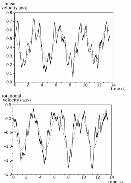
walking along the sides of the square. After filtering out noise (by using dominant frequencies in the power spectrum), we model the translational and rotational velocities as sine waves (see figure 5), as this is a suitable model for a circular motion such as the one observed here.

velocity(m/s)

linear

(s)

0 0.8

0.7

0.6

0.5

0.4

0.3

0.2

0.1

0.0

2 4 6 8 10 12 14 time

0 0.5

0.0

−0.5

−1.0

−1.5

−2.0

2 4 6 8 10 12 14 time velocity

rotational

(rad/s)

(s)

Fig. 5. The demonstrator’s translational and rotational velocities (solid lines), and their filtered counterparts (dashed lines).

We then used the Narmax system identification procedure to obtain two sensor free polynomials, one expressing the linear velocity commands to the robot as a function of past linear velocity commands another expressing the rotational velocity commands to the robot as a function of past ro-tational velocity commands. Both models were chosen to be first degree with regression order 2 in the output (i.e.

l=1,Nu=0,Ny=2) resulting in linear ARMAX structures. Both resulting time series contained 3 terms, and are given in table I.

Having obtained these sensor-free polynomial models, we used them to drive the robot in the square environment (figure 6). During this first robot interaction with the environment,

lv(n) = av(n) = +0.0141 −0.017

+1.966∗lv(n−1) +1.966∗av(n−1)

−1.000∗lv(n−2) −1.000∗av(n−2) TABLE I

MODELS OF TRANSLATIONAL VELOCITYlv(n)INm/sAND STEERING SPEEDav(n)INrad/sAT TIME INSTANTn.

laser readings and the robot’s translational and rotational velocities were logged every 100ms(see also figure 6).

Fig. 6. The trajectory of robot driven by the sensor-free model in the square environment.

a) Sensor signal encoding: In order to decrease the dimensionality of the input space to the Narmax model, we coarse coded the laser readings into 10 sectors by averaging 62 readings for each 24degreeinterval. We then used the Narmax identification procedure to estimate the robot’s translational and rotational velocities as a function of the last three coarse coded laser readings (u8,u9andu10)

found on the left side of the robot (figure 1).

Both models were chosen to be first degree, and no regression was used in the inputs and output (i.e. l=1,

Nu=0,Ny=0), resulting in linear ARMAX structures. Both resulting models contained 4 terms and are given in table II.

lv(n) = av(n) = +0.036 −0.284

+0.246∗u(n,1) +0.685∗u(n,1) −0.106∗u(n,2) −0.440∗u(n,2)

−0.062∗u(n,3) −0.131∗u(n,3) TABLE II

SENSOR BASED MODELS OF TRANSLATIONAL VELOCITYlv(n)INm/s AND ROTATIONAL VELOCITYav(n)INrad/sAT TIME INSTANTn.u1TO

b) Model validation: Finally, having obtained the sensor-based models, we tested the robot in the square envi-ronment (figure 7), as well as in different test envienvi-ronments. The results, given in figure 8, show that the sensor-based models indeed captured the essential relationship between the robot’s perception and its velocity commands to obtain left-hand wall following behaviour.

Fig. 7. The trajectory of robot, driven by the sensor-based models in the square environment.

B. Corridor Passing

In the second experiment, we demonstrated to the robot how to follow a U-shaped a corridor of 150cm width (see figure 9).

We then again obtained two auto regressive models, one expressing the translational velocity as a function of time, another expressing the rotational velocity commands as a function of time and past output commands. The translational speed model was chosen to be second degree with no regression in the input and output ((i.e.l=2,Nu=0,Ny=0). The resulting model contained 3 terms. The steering speed model was chosen to be second degree with regression order 1 in output ((i.e. l=2, Nu=0, Ny=1), and contained 9 terms. Both models are given in table III.

As before, we used the sensor-less models to drive the robot in the U corridor environment. During this time, laser readings and the robot’s translational and rotational velocities were logged every 100ms. This data was then used to obtain the sensor-based models of translational and steering speeds.

c) Sensor signal encoding: Again, in order to decrease the dimensionality of the input space to the Narmax model, we coarse coded the laser readings into 10 sectors by averaging 62 readings for each 24 degree intervals. This time we used all the coarse coded laser readings in Narmax models.

Fig. 8. The trajectories of robot driven by sensor based models in i) 5mx3m

rectangle environment and ii)the environment containing wide and narrow angle corners.

lv(n) = av(n) = +0.347 −0.005

+0.004∗u(n,1) +0.001∗u(n,1)

−0.001∗u(n,1)2 +0.001∗u(n,1)2 −0.001∗u(n,1)3

+0.818∗y(n−1)

+0.158∗y(n−1)2 −0.276∗y(n−1)3 +0.001∗u(n,1)∗y(n−1) −0.001∗u(n,1)2

∗y(n−1) TABLE III

SENSOR-LESS CORRIDOR FOLLOWING MODELS OF TRANSLATIONAL VELOCITYlv(n)(INm/s)AND STEERING SPEEDav(n)(INrad/s)AT

TIME INSTANTn.

Both models were chosen to be first degree and no regression was used in the inputs and output (i.e. l =1,

Nu=0, Ny=0) resulting in linear ARMAX structures. The

lvmodel contained 10 terms and theavmodel contained 9, both models are given in table IV.

lv(n) = av(n) = +1.011 +0.570 −0.037∗u(n,1) +0.002∗u(n,1) +0.164∗u(n,2) +0.069∗u(n,2)

+0.147∗u(n,3) +0.052∗u(n,3) −0.128∗u(n,4) −0.181∗u(n,4)

−0.116∗u(n,5) −0.046∗u(n,5) −0.051∗u(n,6) −0.049∗u(n,6)

−0.075∗u(n,7) −0.038∗u(n,7) −0.051∗u(n,8) −0.020∗u(n,9)

−0.074∗u(n,9) −0.050∗u(n,10) −0.131∗u(n,10)

TABLE IV

SENSOR-BASED SPEED MODELS OF TRANSLATIONAL VELOCITYlv(n)

(INm/s)AND ROTATIONAL VELOCITYav(n)(INrad/s)AT TIME INSTANT n.u1TOu3ARE THE FIRST THREE COARSE CODED LASER READINGS

STARTING FROM THE LEFT EXTREME OF THE ROBOT.

d) Model validation: We then validated the sensor-based models by testing the robot in U corridor environment. The results show that the sensor based models captured the essential relation between the robot’s laser perception and its velocity commands well (see figure 10).

C. Transparent models allow hypothesis postulation and testing

Having transparent models like the one given in table IV has a number of advantages, for example the possibility to analyse robot behaviour formally, or to optimise an existing model in a principled way.

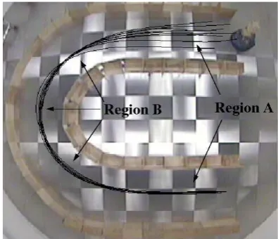
Fig. 10. The trajectories of the robot driven by sensor-based models in the U corridor environment. The robot started from 10 different locations, and in each run it managed to pass the corridor successfully.

e) Behaviour analysis: Transparent mathematical mod-els of behaviour provide an understanding how each robot sensor affects the overall behaviour of the robot. For instance, by looking at the rotational velocity model in table IV, we see that the model has a bias (DC component in the model) of turning to the left. The counterweight terms which balance the bias in the model are terms 5, 6 and 7, which use laser readingsu4,u5andu6respectively.

When the robot is near the right tip of the U corridor (Region A, figure 10), the sensor readings u4, u5 and u6

have high values. Therefore model terms 5, 6 and 7 produce high negative values, which counteract the effect of the DC component so that robot actually moves straight. As the robot approaches the circular part of the corridor (Region B, figure 10) however, these sensor readings become smaller and the DC component begins to dominate the computation of the rotational velocity, making the robot turn left. Once the robot finishes the circular part of the corridor (region A), again sensor readings u4, u5 and u6 have high values and make

the robot go straight until the end of the corridor. Figure 11 illustrates this distribution of steering speeds.

Optimising the model: Further analysis reveals that the rest of the terms, terms 2, 3, 4, 8, 9 and 10, smooth the effects of the terms mentioned above. Once we identified the major terms and therefore the important sensor readings in the model, we were able to used the NARMAX system identification method again to obtain a new, optimised model, expressing the rotational velocity of the robot as a function of only these three major inputs u4, u5 and u6. The new

rotational

time(s)

velocity(rad/s)

Region A Region A Region B

0 5 10 15 20 25 30 35 40 45 −0.05

0.00 0.05 0.10 0.15 0.20

Fig. 11. The rotational velocity of the robot along the U corridor. When the robot is in region A, it has almost no rotational velocity, and therefore moves straight. On the other hand, it has high negative turning velocity, when it is in region B, and turns left.

inputs and the output (i.e.l=1,Nu=0,Ny=0).

We then validated the new model in the test environment. The results show that the performance of the new model is as good as the previous model (see figure 12), but, of course, far more parsimonious.

Fig. 12. The trajectories of robot driven by an optimised model of rotational velocity, using only three inputs. The robot started from 10 different locations and managed to pass the corridor successfully each time.

IV. CONCLUSIONS AND FUTURE WORK

Conclusions: We have shown how the NARMAX mod-elling approach can be used to translate human behaviours al-gorithmically and automatically into robot control code. Ob-taining robot controllers by transforming human behaviours

through system identification does not require any theoretical knowledge in robot programming and is very efficient. Our sensor based models were ready to run within a few hours. The tasks investigated in this paper could have been achieved using other machine learning approaches, such as supervised artificial neural networks (e.g. MLP, RBF, LVQ or support vector machines). However, these approaches can be slow in learning, especially when using large input spaces and, more importantly, generate opaque models that are difficult (if not impossible) to visualise and analyse.

In contrast, our modelling approach producestransparent

mathematical functions that can be directly related to the task. This allows an analysis of how each sensor effects the overall behaviour of the robot. In the example presented here, we demonstrated this fact by identifying the important model terms (and therefore the important sensor signals) in the corridor passing behaviour. We then used only the important sensory inputs to obtain an optimised Narmax model, which performed as well as the previous model, while being even more parsimonious.

Future Work: Not using any sensor signals at all, the initially obtained auto regressive models are sensitive to the robot’s starting position within the environment. Also, they are obviously unable to detect collisions, etc. during the robot’s first run through the environment. We are therefore currently investigating how to combine some basic collision avoidance procedures with the described model identification approach. In particular, we are interested to determine if the obtained models are still fully functional, or if the imprinted, low level collision avoidance behaviour affects the model building process adversely.

V. ACKNOWLEDGEMENTS

We thank to Ali Kutchuk for his contributions to this work. We also gratefully acknowledge that the RobotMODIC project is supported by the Engineering and Physical Sci-ences Research Council under grant GR/S30955/01.

REFERENCES

[Akanyeti et al., 2007] Akanyeti, O., Kyriacou, T., Nehmzow, U., Iglesias, R., and Billings, S. (2007). Visual task identification and characterisation using polynomial models. Robotics and Autonomous Systems. [Billings and Chen, 1998] Billings, S. and Chen, S. (1998). The

deter-mination of multivariable nonlinear models for dynamical systems. In Leonides, C., (Ed.),Neural Network Systems, Techniques and Applica-tions, pages 231–278. Academic press.

[Billings and Voon, 1986] Billings, S. and Voon, W. S. F. (1986). Corre-lation based model validity tests for non-linear models. International Journal of Control, 44:235–244.

[Demiris and Hayes, 1996] Demiris, J. and Hayes, G. (1996). Imitative learning mechanisms in robots and humans. In Proc. 5th European Workshop on Learning Robots, pages 9–16, Bari, Italy.

[Hayes and Demiris, 1994] Hayes, G. and Demiris, J. (1994). A robot controller using learning by imitation. InProc. 2nd Int. Symposium on Intelligent Robotics Systems, pages 198–204, Grenoble, France. [Iglesias et al., 2005] Iglesias, R., Kyriacou, T., Nehmzow, U., and

Billings, S. (2005). Robot programming through a combination of manual training and system identification. In Proc. of ECMR 05 -European Conference on Mobile Robots 2005.Springer Verlag. [Korenberg et al., 1988] Korenberg, M., Billings, S., Liu, Y. P., and

McIl-roy, P. J. (1988). Orthogonal parameter estimation algorithm for non-linear stochastic systems.International Journal of Control, 48:193–210. [Roberto Iglesias and Billings, 2005] Roberto Iglesias, Ulrich Nehmzow, T. K. and Billings, S. (2005). Modelling and characterisation of a mobile robot’s operation. Santiago de Compostela, Spain.

[Schaal, 1997] Schaal, S. (1997). Learning from demonstration. In