Distributed representations accelerate evolution of adaptive behaviours

promoting access to White Rose research papers

White Rose Research Online

Universities of Leeds, Sheffield and York

http://eprints.whiterose.ac.uk/

This is an author produced version of a paper published in PLoS Computational Biology.

White Rose Research Online URL for this paper: http://eprints.whiterose.ac.uk/3452/

Published paper

Distributed Representations Accelerate

Evolution of Adaptive Behaviours

JV Stone,

Psychology Department, Sheffield University, England, S10 2TP.

Tel: (0) 114 2226522, fax: (0) 114 276 6515

Email:

[email protected]

Running head: Accelerated Evolution.

Abbreviations: FLL: free-lunch learning.

Abstract

Animals with rudimentary innate abilities require substantial learn-ing to transform those abilities into useful skills, where a skill can be

considered as a set of sensory-motor associations. Using linear neural network models, it is proved that, if skills are stored as distributed

rep-resentations, then within-lifetime learning of part of a skill can induce automatic learning of the remaining parts of that skill. More

impor-tantly, it is shown that this ‘free-lunch’ learning (FLL) is responsible for accelerated evolution of skills, when compared to networks which

either, 1) cannot benefit from FLL, or 2) cannot learn. Specifically, it is shown that FLL accelerates the appearance of adaptive behaviour,

both in its innate form and as FLL-induced behaviour, and that FLL can accelerate the rate at which learned behaviours become innate.

Synopsis

Some behaviours are purely innate (e.g. blinking), whereas other, apparently ‘innate’,

behaviours require a degree of learning to refine them into a useful skill (e.g. nest

building). In terms of biological fitness, it matters how quickly such learning occurs,

because time spent learning is time spent not eating, or time spent being eaten, both of

which reduce fitness. Using artificial neural networks as model organisms, it is proven

that it is possible for an organism to be born with a set of ‘primed’ connections which

guarantee that learning part of a skill induces automatic learning of the remaining skill

components, an effect known as free-lunch learning. Critically, this effect depends on

the assumption that associations are stored as distributed representations. Using a

genetic algorithm, it is shown that primed organisms can evolve within 20 generations.

This has three important consequences. First, primed organisms learn quickly, which

increases their fitness. Second, the presence of free-lunch learning effectively accelerates

the rate of evolution, for both learned and innate skill components. Third, free-lunch

learning can accelerate the rate at which learned behaviours become innate. These

findings suggest that species may depend on the presence of distributed representations

1

Introduction

Both evolution and learning may be considered as different types of adaptation.

Learn-ing occurs within a lifetime, whereas genetic change occurs across lifetimes [1]. Whereas

genetic change ensures that a task can be executed innately, learning permits even the

most rudimentary innate ability to be honed into a useful skill.

In an environment which fluctuates from generation to generation, learning permits an

innate ability to be adapted to the particular physical environment into which each

generation is born. If the environment ceases to fluctuate then genetic assimilation

[2] can transform a rudimentary innate ability which requires much learning into an

innate skill which requires minimal learning. This transformation is more likely to

occur if the cost of learning is high [3, 4], and, in this case, computer simulations

suggest that learning can accelerate the rate of genetic assimilation [5] via the Baldwin

effect [6]. However, if learning is sufficiently inexpensive then genetic change may not

occur at all [7, 8]. Overall, there appears to be a trade-off between learning and genetic

assimilation, such that learning can subsidize genetic change, especially if learning is

inexpensive.

All but the most primitive organisms learn in order to survive, and organisms which

learn quickly are at a selective advantage relative to those that learn slowly. Therefore,

a mechanism which reduces the time required to learn a given behaviour confers a

selective advantage. One candidate for such a mechanism is free-lunch learning (FLL)

[9],[10].

As explained below, FLL ensures that, in the process of learning one set of associations

or behaviours, another set of associations is usually learned. These associations could

comprise either perceptual skills (such as face recognition, predator recognition [11] or

prey recognition), or motor skills (such as catching prey, flying, seed pecking, or nest

1.1

Free-Lunch Learning

Before considering how FLL can accelerate evolution of certain types of behaviours,

FLL will be described in its original context of spontaneous recovery of memory in

humans [9] and in neural network models [10]. Note that FLL is not unique to a

specific class of network architectures, although it does assume that associations are

learned using a form of supervised learning.

In humans, FLL has been demonstrated using a task in which participants learned

the positions of letters on a non-standard computer keyboard [9]. After a period of

forgetting, participants relearned a proportion of these letter positions. Crucially, it

was found that this relearning induced recovery of the non-relearned letter positions.

More recently, a set of theorems provided a formal characterization of FLL in linear

neural network models [10]. In essence, FLL occurs in neural network models because

each association is distributed amongst all connection weights (synapses) between units

(model neurons). After partial forgetting, relearning some of the associations forces

all of the weights closer to pre-forgetting values, resulting in improved performance

even on non-relearned associations; a general proof is provided in [10]. A geometric

demonstration of FLL for a network with two connection weights is given in Figure

2. Networks with multiple input and output units can be considered without loss of

generality [10].

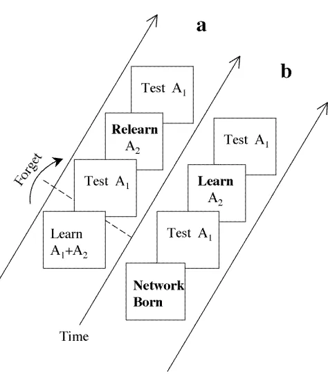
The protocol used to examine FLL in neural networks is as follows (see Figure 1). A

network withninput units and one output unit hasnconnection weights. This network

learns a set A of m ≤ n associations, where A = A1∪A2 comprises two subsets A1

and A2 of n1 and n2 associations, respectively (note that m = n1 +n2). After the

associations A have been learned and then partially forgotten, performance error on

subset A1 is measured (forgetting is induced by adding isotropic noise to weights).

Finally, only A2 is relearned and then performance error on A1 is re-measured. FLL

occurs if relearning A2 improves performance on A1. It has been proven that the

probability of FLL approaches unity as the number of weights increases [10]. For

performance on A2”, in this paper.

1.2

FLL and Evolution

Now consider an organismb2 which is born with a genetically specified set of neuronal

connections [12]. These connections are organised such that, if b2 learns one subset A2

of associations then another subsetA1 is usually learned. In other words,the organism

b2 is born with neuronal connections similar to the connections of an organismb1 which

had once learned and then forgotten subsets A1 and A2 (e.g. isotropically distributed

aroundw0in Figure 2). Just as FLL ensures that if organismb1 relearnsA2then subset

A1 is usually relearned (see Figure 1), so if b2 learns A2 then A1 is usually learned.

In both cases, FLL ensures that learning one subset of associations induces learning

of the other subset. Critically, whereas the FLL exhibited by organism b1 depends on

previous learning and forgetting, FLL in organismb2 depends on being born in a state

such that the first time A2 is learned, the associationsA1 are also usually acquired. A

more formal account of this effect is given in the next section.

The use of two distinct subsets in this paper is clearly unrealistic when considered

in the context of skill learning. However, the use of two subsets lies at one extreme

along a continuum of tasks. At one extreme, associations are learned one by one in a

strict order, and at the other extreme, all associations are learned simultaneously. In a

biological context, the components of a skill which are learned first act as ‘scaffold’ for

others, and this effectively imposes a temporal order to the acquisition of different skill

components. This is the type of scenario assumed for the simulations reported in this

paper. Essentially, learning A2 is assumed to consist of a subset of skill components

which provide a scaffold for the skill components in A1.

2

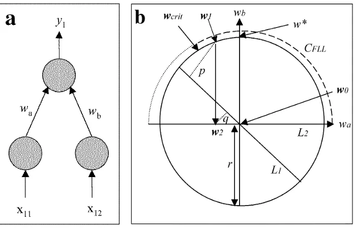
The Geometry of FLL

This section is a brief account of the basic geometry underlying FLL, in the absence of

we assume that the network has one output unit and two input units, which implies

n= 2 connection weights, and thatA1 and A2 each consist of n1 =n2 = 1 association,

as in Figure 2. Input units are connected to output unit via weights wa and wb,

which define a weight vector w= (wa, wb). AssociationsA1 and A2 consist of different

mappings from the input vectors x1 = (x11, x12) and x2 = (x21, x22) to desired output

values d1 and d2, respectively. If a network is presented with input vectors x1 and x2

then its output values arey1 =w·x1 =wax11+wbx12and y2 =w·x2 =wax21+wbx22,

respectively. More generally, network performance error for k associations is defined

as

E(w, A) =

k

X

i=1

(di−yi)2. (1)

The weight vector w defines a point in the (wa, wb)-plane. For an input vector x1

there are many different combinations of weight valueswaand wb that give the desired

output d1. These combinations lie on a straight line L1, because the network output

is a linear weighted sum of input values. A corresponding constraint line L2 exists for

A2. The intersection of L1 and L2 therefore defines the only point w0 that satisfies

both constraints, so that zero error on A1 and A2 is obtained if and only if w= w0.

Without loss of generality, we define the origin w0 to be the intersection of L1 and L2.

A general prerequisite for FLL is thatL1 is not orthogonal to L2.

We now consider the geometric effect of partial forgetting of both associations, followed

by relearning A2. This geometric account applies to a network with two weights (see

Figure 2), and depends on the following observation: if the length of the input vector

kx1k= 1 then the performance error E(w, A1) = (d1 −y1) 2

of a network with weight

vector w when tested on association A1 is equal to the squared distance between w

and the constraint line L1 [10]. For example, if w is in L1 then E(w, A1) = 0, but as

the distance betweenw and L1 increases soE(w, A1) must increase. For the purposes

of this geometric account, we assume that kx1k=kx2k= 1.

If partial forgetting is induced by adding isotropic noisegto the weight vector w=w0

then this effectively moveswto a randomly chosen pointw1 =w0+gon the circleC of

w1, learningA2moveswto the nearest pointw2onL2 [10], so thatw2is the orthogonal

projection of w1 on L2. Before relearning A2, the performance error E(w1, A1) on A1

is the squared distance p2

between w1 and its orthogonal projection on L1. After

relearning A2, the performance error Epost is the squared distance q2 between w2 and

its orthogonal projection on L1. The amount of FLL is δ = E(w1, A1)−E(w2, A1),

and (for a network with two weights) is also given by Q = p2

−q2

. The probability

P(δ >0) of FLL given L1 and L2 is equal to the proportion of points on C for which

δ >0 (or equivalently, for which Q >0). For example, it can be shown that the mean

value of this proportion isP(δ >0) = 0.68 for a two-weight network like the one shown

in Figure 2a. Given the particular configuration shown in Figure 2a, the critical point

wcrit is defined such that the performance error before and after learning is the same

(i.e. δ = 0).

3

FLL Induces Perfect Performance

Given a network withnweightswand two subsetsA1 andA2 ofn1 andn2associations,

respectively, it is shown that weights w∗ _{exist such that learning associations A2 is}

guaranteed to yield zero performance error on A1, provided n ≥n1+n2.

Consider a network withn = 2 weights and subsetsA1 andA2 each of which comprises

a single association. Each association defines a constraint lineL1 and L2, respectively

(see Figure 2). If the weight vector w is in L1 then performance error on A1 is zero,

and if w is inL2 then performance error on A2 is zero. Clearly, if and only if w is at

the intersection w0 of L1 and L2 then performance error on both A1 and A2 is zero.

Ifw is not in L2 then learning A2 moves w from its current position to its orthogonal

projection ontoL2 [10]. Crucially, if w=w∗ in Figure 2 then learning A2 moves wto

the optimal weight vector w0. In this case, learning A2 reduces performance error to

zero on both A1 andA2, and therefore learningA2 implies perfect performance on A1.

This line of reasoning generalises to networks with more than two weights, as follows.

and n2 >1 associations. Ifn≥n1+n2 thenA1 andA2 define an (n−n1)-dimensional

subspaceL1 and an (n−n2)-dimensional subspaceL2, respectively. The intersectionL12

of L1 and L2 corresponds to weight vectors which generate zero error onA=A1∪A2.

In this case, the circle in Figure 2 corresponds to an n-dimensional hypersphere, with

its centre w0 in L12. Given that learning A2 provides an orthogonal projection of w

onto L2, and that there exists a w = w∗ such that its orthogonal projection onto L2

is w0, it follows that learning A2 in a network with w = w∗ yields zero performance

error on both A2 and A1.

Given that the weight vector wis genetically specified with finite precision, a network

is necessarily born with its weight vector w = w1 at a non-zero distance r from the

optimal weight vector w0. This finite precision defines a hypersphere C around w0,

and the location ofw1 onC determines the amount of FLL. If a network is born with

w1 = w∗ then learning A2 induces perfect performance on A1. If fitness depends on

performance on both A1 and A2 after learning only A2 then there is selective pressure

for networks to be born with weight vectors close to w∗_{, given a specific degree of}

genetic precision r. More generally, there is pressure for networks to be born with

weight vectors on the line which passes through w0 and w∗.

3.1

Terminology: Evolution, Innateness and FLL

As this paper deals with subtle combinations of evolution and learning, involving two

distinct subsets of associations (A1 and A2), it is important to be clear about

termi-nology. Specifically, we need to be careful about which subset is being referred to, and

whether we are referring to innate performance or not. Accordingly, performance error

on A1 before learning A2 is called just that, ‘innate performance error on A1’.

Be-haviours which are induced by learningA2 are calledFLL-inducedbehaviours, because

they are not innate, nor are they learned, so that performance error onA1 after

learn-ing A2 is called ‘FLL-induced performance error on A1’. If learning A2 does not affect

performance on A1 (as in condition NoFLL, below) then this is referred to as

context (e.g. performance on A1 after learning A2).

4

Methods

The effect of FLL on evolution was tested by measuring performance on A1 after

learning A2 across generations. In order to eliminate the possibility that the observed

results are artefacts, the effects of FLL were compared with two control conditions

(described below).

Each generation consisted of 1000 neural networks, each of which consisted of 20 input

units and one output unit. The genome of each network was defined by a one-to-one

mapping of then= 20 weight values in the network to a single string ofn genes, where

the value of each gene was set to the value of a corresponding network weight. The

number of offspring generated by each network was proportional to its fitness, which

depended only on its ability to provide the correct desired output value for each of

20, n-element input vectors. The mapping from each input vector to its output value

defines one association (see Figure 2).

A network’s output yi is a weighted sum of input values yi = w·xi = Pn1

+n2

j=1 wjxij, where xij is the jth value of the ith input vector xi, and each weight wi is one

input-output connection.

The fitness of each network was assessed with respect to its performance error on a

single common set A = (A1 ∪A2) of m = 20 associations, where A1 and A2 are two

disjoint subsets of n1 = 10 and n2 = 10 associations, respectively. The m associations

in A were allocated randomly to the two subsets, A1 and A2. The subsets A1 and A2

were intended to represent different components of a task, and were therefore the same

for all networks, and across all generations. In the first generation, each network’s

weight values were chosen from a gaussian distribution (see below for details).

The desired output value di for each input vector xi was drawn from a gaussian

dis-tribution with variance 1/n. An analytic method was used to solve for the optimal

variances of the inputs and outputs, the expected length of w0 is unity.

Each new generation was formed from 1000 matings between 1000 pairs of networks.

TheKth network was chosen for mating according to its fitnessF(K) with probability

p(K). Networks were chosen with replacement to ensure that the number of offspring

from a given network was proportional top(K). The probability p(K) was defined as

p(K) = _P1000F(K)

k F(k)

, (2)

where the denominator ensures P

kp(k) = 1. Half the weights of each offspring were

copied from (randomly chosen) corresponding weight locations in one parent network,

and half from the other parent. Aside from mutations, weight values inherited by

an offspring were the same as those inherited by its parents (i.e. inheritance was

Darwinian, not Lamarckian).

Mutation was applied to each weight with a probability of 0.05, using a uniform

prob-ability density function. Then gaussian noise with a standard deviation of 0.05 was

added to the value of those weights which had been chosen for mutation.

There were three conditions: FLL, NoFLL, and NoLearn, with corresponding fitness

functionsFF LL, FN oF LL, and FN oLearn. The initial randomly chosen weight values (see

Network Learning Algorithm) of the population of networks were the same in each

condition. Networks were selected for mating according to their performance on the

combined set A = (A1 ∪A2), according to Equation (2) for all fitness functions, as

described next.

Condition FLL: Networks which exhibited high levels of FLL were preferentially

selected for mating. Only associationsA2 were learned, but the fitness of each network

depended on its performance on both the learned associationsA2 and on the unlearned

associations A1. The fitness FF LL(K) of the Kth network is defined in terms of its

innate performance errorEpre onA= (A1∪A2), and on its performance errorEpost on

A after learning A2:

FF LL(K) =

1

cEpre+ (1−c)Epost

where

Epre =

n1+n2

X

i

Dpre_i (4)

Epost =

n1+n2

X

i

Dpost_i ≈

n1

X

i

D_ipost, (5)

whereDpre_i and Dpost_i are the network’s output errors in response to the ith input

vec-tor before and after learning A2 (respectively). The parameter c = 0.05 defines the

balance between performance error on innate versus post-learning (e.g. FLL-induced)

behaviours, and is interpreted as a cost-of-learning parameter (see below). The

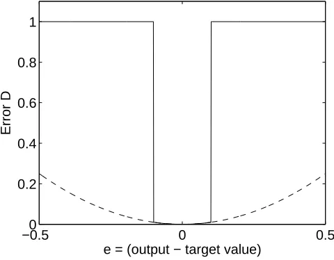
net-work’s fitness error Di is a function of the differenceei =yi−di between the network’s

response yi to the ith input vector and the desired output value di:

Di =

     e2

i if e

2

i ≤Dthresh ,

1 if e2

i > Dthresh .

(6)

This ensures that output errors above Dthresh have a disproportionately large and

detrimental effect on fitness, as shown in Figure 3. This, in turn, ensures that only

those networks with ‘good’ performance are likely to be selected for reproduction. The

value ofDthresh was set to 0.01.

For later use, we also define the fitness errors Epre =Epre(A1) +Epre(A2), andEpost =

Epost(A1) +Epost(A2) ≈ Epost(A1). The approximation here and in Equation (5)

em-phasises the fact that the total fitness error is attributable almost exclusively to A1

after learning A2 (because error on A2 is then almost zero).

The inclusion of innate performance errorEpre inFF LLensures that the cost of learning

is taken into account when assessing fitness. If c is small then Epre tends to be large,

so that much learning is required to increase fitness. Conversely, if cis large then Epre

tends to be small, so that little learning is required to increase fitness. Thus Epre is

an implicit measure of the cost of learning (where cmultipliesEpre), and ensures that

networks which require minimal learning have high innate fitness (although the small

Condition NoFLL: This was identical to condition FLL, except that the effects of

FLL were precluded by making L1 and L2 orthogonal. This ensures that learning A2

cannot affect performance on A1. Orthogonality was achieved by making all input

vectors in A mutually orthogonal, whilst retaining the length of each vector as in

condition FLL, using Gram-Schmidt orthogonalisation. The fitness function FN oF LL

was the same as in condition FLL (i.e. FN oF LL=FF LL).

Condition NoLearn: No learning occurred, so that improvement in performance over

successive generations was due only to selection of innate performance on A1 and A2.

Fitness was defined as FN oLearn= 1/Epre, whereEpre is defined in Equation (4). This

is equivalent to setting c= 1 in Equation 3.

Network Learning Algorithm: The network learning algorithm used here involves

a type of supervised learning. Note that Equation (1) defines the network error used

for learning, whereas Equation (3) defines the fitness of a network.

Each network was initialised with n weight values drawn randomly from a gaussian

distribution with unit variance. This was then divided byn1/2

, which ensures that the

expected length of weight vectors in the population is unity.

Given a network with n input units and one output unit, the set A of m, n-element

input vectors xi :i= 1. . . m and m desired scalar output target valuesdi were chosen

randomly from a gaussian distribution with unit variance. Each input vector was then

divided byn1/2

so that the expected length of input vectors was unity (i.e. the variance

of input values was 1/n).

In conditions FLL and NoFLL each network learned n2 associations. Rather than

using the iterative weight update normally associated with the delta rule, an analytic

solution was obtained. Learning n2 associations consists of finding the orthogonal

projection operator which projects the initial weight vector w1 to its nearest point in

the subspace (e.g. L2) defined by the n2 input vectors being learned. The end result

w2 is the same as that obtained using the standard delta rule for infinitesimal learning

rates [10]. As with the standard delta rule, this yielded a value of approximately

learning is most plausibly associated with motor learning in the cerebellum and basal

ganglia [10].

5

Results

The results are based on 10 computer simulation runs for each of the three conditions

FLL, NoFLL, and NoLearn, described above, and graphs show the mean of these 10

runs. Each run involved a different fixed set A of 20 associations. As a reminder, the

two free parameters are: 1) the cost-of-learning parameter, which was set to c= 0.05,

and, 2) the threshold of the fitness error function , which was set to Dthresh = 0.01.

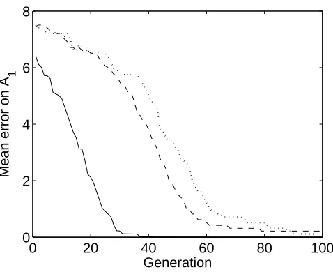
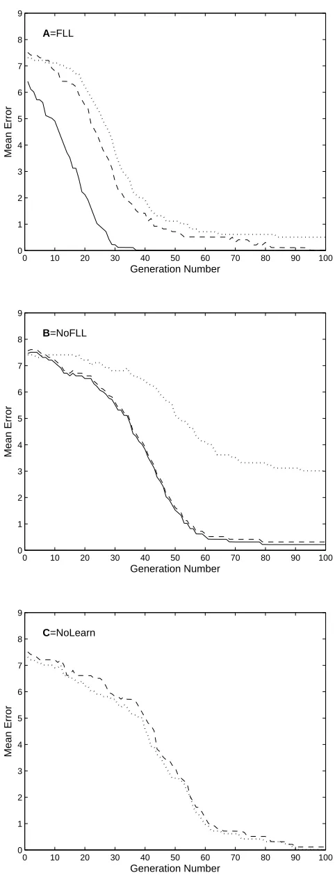
The main results are shown in Figure 4, which is a summary of more detailed results in

Figure 6. Condition FLL yields a FLL-induced error (i.e. error onA1 after learningA2)

of approximately zero after 21 generations, whereas condition NoFLL requires around

60 generations to achieve an error of less than unity. Condition NoLearn (dotted curve)

yields the slowest innate learning, and is included for comparison.

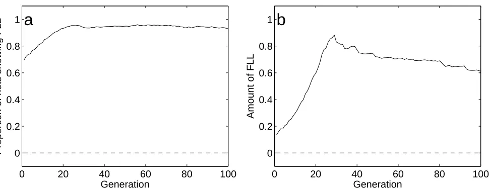
The proportion of networks which exhibit FLL over generations is shown in Figure

5a, and the amount of FLL is shown in Figure 5b. The proportion and amount of

FLL increases in condition FLL, as indicated by the solid line in each figure. The zero

prevalence of FLL in condition NoFLL (dashed line) is associated with zero FLL as

indicated in Figure 5b. More detailed results are shown in Figure 6a-c.

Performance on A1 : Performance onA1 (solid line in Figure 6a) after learningA2 is

better in condition FLL than in condition NoFLL (solid line, 6b). Innate performance

on A1 is also better in condition FLL (dashed line, 6a) than in conditions NoFLL

(dashed line, 6b) and NoLearn (dashed line, 6c). Together, these results suggets that

FLL accelerates both the rate at which FLL-induced behaviours (A1) appear, as well

as the rate at which FLL-induced behaviours (A1) become genetically assimilated.

Performance on A2: Innate performance on subset A2 is better in condition FLL

(dotted curve in Figure 6a) than in conditions NoFLL (dotted curve, 6b) and NoLearn

LearningA2 reduces error on subset A1 even in the first generation in conditions FLL

(Figure 6a). Additionally, the proportion of networks showing FLL is greater than

0.5 (Figure 5a), and the amount of FLL is greater than zero (Figure 5b) in the first

generation. These effects are not due to any special properties of the networks nor

of the associations. Indeed they are entirely expected, and are consistent with the

theoretical analysis in [10]. In essence, FLL is observed in the first generation because

it is very unlikely that the mainfoldsL1 andL2 defined byA1 andA2 (respectively) are

orthogonal, so that learning A2 usually reduces error onA1 (albeit by a small amount

in the first generation).

6

Discussion

Before discussing results in detail, it is important to clarify precisely what is being

claimed here. The main claim is that, given a population of organisms which can learn,

the presence of FLL accelerates the rate at which a given set of advantageous behaviours

evolves relative to populations which, 1) can learn but which do not have FLL (e.g.

condition NoFLL), and, 2) cannot learn (e.g. condition NoLearn). Specifically, it is

claimed that FLL accelerates the appearance of adaptive behaviour, both in its innate

form and as FLL-induced behaviour, and that FLL can accelerate the rate at which

learned behaviours become innate.

It is also claimed that FLL increases the rate at which a set of behaviours (e.g. A) is

acquired within a lifetime. Clearly, if learning one subset (e.g. A2) induces learning of

another subset (e.g. A1) then the amount of learning required to learn both subsets

(e.g. A) is reduced.

It is worth noting that FLL is not related to generalisation (see [10]), and the effects

6.1

Task Difficulty

The task was purposely made difficult, such that network outputs which were not

close to desired target values were assigned an error value of unity. This heavily

penalises networks which do not generate near-correct responses. This type of task

may emulate tasks for which being ‘almost correct’ provides no fitness benefit. Such

tasks are exemplified by a predator which almost catches prey (e.g. a kingfisher almost

catching a fish, or where each failed attempt yields a large fitness cost), or where

learning is incremental and step-wise (e.g. learning to catch progressively larger prey).

Such tasks may give rise to ‘needle-in-a-haystack’ search spaces [5], which have rugged

or uncorrelated landscapes [13].

6.2

Is Accelerated Evolution Due To Learning?

A cogent critique of research by Nolfi et al [14] argues that accelerated evolution

(assimilation) is a generic consequence of learning per se [15]. In results not shown

here, replacing A2 with a new, randomly chosen subset every generation in condition

FLL yields a more gradual evolution of FLL-induced and innate behaviours than is

obtained in any of the conditions used here. This effectively excludes the possibility

that the accelerated evolution reported here is due to learningper se.

6.3

Reaction Norms

In terms of evolutionary theory, FLL-induced behaviours can be considered as the

establishment of a new reaction norm. The specific ‘environment’ that induces the

reaction norm is learning a particular subset of behaviours (A2), and the phenotypic

6.4

Genetic Assimilation

FLL does not necessarily force FLL-induced behaviours to become genetically

assimi-lated. In fact, there is a trade-off between the amount of acceleration induced by FLL

and the extent to which behaviours become innate. If the cost-of-learning parameter is

set toc= 1 then there is no incentive for FLL to increase over generations. In contrast,

if c≈0 (as in the simulations reported here) then the rapid evolution of FLL-induced

behaviour shown in Figure 6a (solid line) is obtained, alongside the slower evolution

of innate behaviour (dashed line in Figure 6a). Thus, even the small value of c (0.05)

used here puts pressure on learned behaviours to become innate, as indicated by the

decreasing innate performance errors onA1 (dashed line) andA2 (dotted line) in Figure

6a.

In practice, learning always has a non-zero fitness cost, if only in terms of the time

required for that learning to occur. This is because time spent learning is time spent

not eating, or time spent being eaten, both of which reduce fitness. Thus, the small

value of c used here represents one value along the spectrum of learning costs. It

therefore seems likely that even the simplest learned behaviours have a tendency to

become innate, and that this tendency increases with the cost of learning. For example,

in results not shown here, increasing the cost-of-learning parametercdecreases the rate

at which FLL-induced performance on A1 improves, and increases the rate at which

performance onA1 andA2becomes innate (innate performance withc= 1 is effectively

obtained in condition NoLearn (see Figure 6c)). It is therefore not easy to classify the

effect reported here as a clear-cut example of the Baldwin effect, although these effects

are almost certainly related.

6.5

General Free-Lunch Effects

The basic geometry which underpins FLL within a lifetime (as in [10]) and across

lifetimes (as here), can also be applied in two other contexts: 1) evolution of innate

cases are considered in the next two paragraphs. Both of these effects require the

presence of environmental conditions which fluctuate over successive generations (e.g.

fluctuations in temperature induced by ice ages, salinity, prey numbers, or predation

pressure).

1) Accelerated evolution of innate behaviours without learning can be understood by

considering an organism which has no learning ability, and which relies on genetic

specification of its neuronal connections [12]. Natural selection ensures that its

neu-ronal connections at birth yield innate behaviour matched to its environment. If the

environment changes then natural selection will induce a corresponding shift to a new

set of innate connections. If the environment then shifts back to its original state then

organisms’ connections will tend to revert to their original values. Let us assume that

some connections revert faster than others over successive generations. For example,

some connections may be specified by genes linked to other innate behaviours, and

this genetic linkage would tend to reduce the rate of genetic change. In fact, for

sim-plicity, assume that half of the connections revert quickly, and half revert slowly. If

the required behaviours are encoded as distributed representations then this

connec-tion reversion will induce a FLL-type effect, such thatallassociations benefit from the

reversion of a proportion (half here) of connection values.

2) Accelerated evolution of general phenotypic traits can be understood if we assume

an extreme form of pleiotropy: that each of a given set of genes affects every phenotypic

trait. This is equivalent to assuming that the genome is a distributed representation

of the phenotype. Consider a population in which the fittest organism has a genome

w0 which is perfectly adapted to its environment e0. If the environment changes to

e1 then the fittest organism’s genome will eventually evolve to a new state w1 that

is suited to e1 (this is analogous to forgetting in FLL). Now, consider what happens

if the environment changes back to e0. The fittest organism’s genome will be forced

back toward w0, but inevitably some genes will revert faster than others. For the sake

of argument, assume that a subset G2 of genes revert to their original values, while

each gene in G2 contributes to every phenotypic trait, the reversion of genes in G2

to their original values will push the entire phenotype back toward its state in the

original environment e0. Thus, the reappearance of an entire set of phenotypic traits

(e.g. changes in size) can occur more quickly if those traits are encoded within a set

of pleiotropic genes than if each trait is represented by a non-pleiotropic gene, and

suggests a form of free-lunch evolution.

7

Conclusion

It has been demonstrated that FLL accelerates the evolution of behaviours in neural

network models. Given that FLL appears to be a fundamental property of distributed

representations, and given the reliance of neuronal systems on distributed

representa-tions, FLL-induced behaviours may constitute a significant component of apparently

innate behaviours (e.g. nest-building). Results presented here suggest that any

organ-ism that did not take advantage of such a fundamental and ubiquitous effect would be

at a selective disadvantage. Finally, if FLL accelerates evolution in the natural world

then it may have been involved in the Cambrian explosion, an explosion that began

when brains (and therefore learning) first appeared.

Acknowledgements: Thanks to N Hunkin and R Lister for comments on this paper,

and to P Parpia for useful discussions. Thanks also to two anonymous reviewers for

References

[1] Bateson G (1979) Mind and Nature. Flamingo.

[2] Waddington C (1959) Canalisation of development and genetic assimilation of

acquired characters. Nature 183:1654–1655.

[3] Mery F, Kawecki T (2003) A fitness cost of learning in drosophila melangaster.

Proc Roy Soc London, B 270:2465–2469.

[4] Price T, Qvarnstrom A, Irwin D (2003) The role of phenotypic plasticity in driving

genetic evolution. Proc Roy Soc London, B 270:1433–1440.

[5] Hinton G, Nowlan S (1987) How learning can guide evolution. Complex Systems

1:495–502.

[6] Baldwin J (1896) A new factor in evolution. The American Naturalist 30.

[7] Mery F, Kawecki T (2004) The effect of learning on experimental evolution of

resource preference in drosophila melangaster. Evolution 58:757–767.

[8] Dopazo H, Gordon M, Perazzo R, Risau-Gusman S (2001) A model for the

inter-action of learning and evolution. Bull Math Biol 63:117–134.

[9] Stone J, Hunkin N, Hornby A (2001) Predicting spontaneous recovery of memory.

Nature 414:167–168.

[10] Stone J, Jupp P (2007) Free-lunch learning: Modelling spontaneous recovery of

memory. Neural Computation 19:194–217.

[11] Tinbergen N (1951) The Study of Instinct. Oxford University Press.

[12] Kaufman A, Dror G, Meilijson I, Ruppin E (2006) Gene expression of

caenorhab-ditis elegans neurons carries information on their synaptic connectivity. PLoS

[13] Kauffman S, Levin S (1987) Towards a general theory of adaptive walks on rugged

landscapes. J Theor Biol 128:11–45.

[14] Nolfi S, Elman J, Parisi D (1994) Learning and evolution in neural networks.

Adaptive Behavior 3:5–28.

[15] Harvey I (1996) Relearning and evolution in neural networks. Adaptive Behaviour

Figure 1: Free-Lunch Learning Within and Across Generations. a) FLL within

the single lifetime of a neural network model. Two subsets of associationsA1andA2are

learned. After partial forgetting (see text), performance error on subsetA1 is measured.

SubsetA2 is then relearned, and performance error on subsetA1 is measured again. If

performance error on A1 decreases as a result of learning A2 then free-lunch learning

(FLL) has occurred. b) FLL across generations. Using a genetic algorithm, a network

is born with connections similar to those of the network in a after it has learned and

then partially forgotten subsetsA1 andA2. Consequently, innate performance error on

A1 is similar to that of the network ina after it has partially forgotten both subsets.

After measuring performance error onA1 at birth, subsetA2 is learned for the first time

by an individual organisms, and performance error on subset A1 is measured again.

After many generations, the innate connection values of each network ensure that if

subset A2 is learned for the first time then this induces automatic learning of subset

Figure 2: Geometry of Free-Lunch Learning. a) Given a network with two input

units and one output unit, its connection weights wa and wb define a weight vector

w= (wa, wb). The network learns two associationsA1andA2, whereA1 is the mapping

from input vector x1 = (x11, x12) to desired output value d1. Learning consists of

adjusting w until the network output y1 = w·x1 equals d1. b) Each association A1

and A2 defines a constraint line L1 and L2, respectively. The intersection of L1 and

L2 defines a point w0 which satisfies both constraints, so that zero performance error

onA =A1∪A2 is obtained if w=w0. After partial forgetting, the weight vector is a

randomly chosen pointw1 on the circleC of radiusr, and the performance error onA1

is given by the squared distance p2

. After relearning A2, the weight vector w2 lies in

L2, and performance error onA1 is the squared distanceq2. FLL occurs if performance

error on A1 is decreased by relearning A2, or equivalently if p2 > q2. Relearning A2

has three possible effects, depending on the position of w1 onC: 1) if w1 is under the

larger (dashed) arc CF LL as shown here then p2 > q2, therefore FLL is observed, 2) if

w1 is under the smaller (dotted) arc, then p2 < q2, therefore negative FLL is observed,

and, 3) if w1 is at the critical point wcrit, then p2 =q2, therefore no FLL is observed.

Given that w1 is a randomly chosen point on the circle C, the probability of FLL is

equal to the proportion of the upper semicircle under the (dashed) arc CF LL. Note

−0.50 0 0.5 0.2

0.4 0.6 0.8 1

e = (output − target value)

Error D

Figure 3: Network fitness error function. The response of the network to a given

input vector x is y =w·x. Given a desired (target) output d, the solid curve shows

how the fitness penalty D for an incorrect response increases sharply (to unity) if the

magnitude of the difference e = y− d is greater than 0.1 (i.e. if e2

> 0.01). For

comparison, the quadratic error function e2

= (y −d)2

, which is minimised during

learning, is shown as a dashed curve. The range of e-values shown are typical for the

0 20 40 60 80 100 0

2 4 6 8

Generation

Mean error on A

1

Figure 4: Effect of free-lunch learning on performance error. The graph shows

the mean results of 10 computer simulation runs, in three conditions FLL, NoFLL, and

NoLearn (see text). In each run, the fitness of each of 1000 networks was determined

by performance error on a fixed setA= (A1∪A2) of 20 associations; a different set A

was used for each run. For all graphs in this paper, the median (of error, here) of 1000

networks was obtained throughout each run, and the mean of 10 medians is shown for

each generation in each condition (standard errors were no greater than 0.5, and are

not shown for clarity).

Condition FLL(solid line): Mean performance errorEpost(A1) on the 10 associations

in A1 after learning the 10 associations in subset A2. Learning A2 had a beneficial

effect on performance on A1 over 100 generations, corresponding to an increase in the

amount and prevalence of FLL (see Figure 5).

Condition NoFLL (dashed line): Mean performance error Epost(A1) was evaluated

as in condition FLL, except that the input vectors in A1 were orthogonal to those in

A2, so that learning A2 could not have any effect on performance on A1 (see text).

Condition NoLearn(dotted line): Mean performance errorEpre onA1 was evaluated

0 20 40 60 80 100 0

0.2 0.4 0.6 0.8 1

Generation

Proportion of nets showing FLL

a

0 20 40 60 80 100 0

0.2 0.4 0.6 0.8 1

Generation

Amount of FLL

b

Figure 5: Prevalence and amount of free-lunch learning. The lines in each graph

correspond to the conditions: FLL=solid line, NoFLL=dashed line. Performance

error on A1 was tested after learning A2 in conditions FLL and NoFLL. Each plotted

line is the mean of 10 computer simulation runs (see Figure 4 for details).

a) Prevalence of FLL: The proportion of networks which showed improved

perfor-mance on A1 after learning A2. In condition FLL, the prevlance FLL was non-zero in

the first generation, as expected (see text), and increased across subsequent

genera-tions. In condition NoFLL, the prevalene remained at zero, as expected.

b) Amount of FLL: In condition FLL, the amount of FLL increased dramatically

over the first 30 generations. The absence of FLL in condition NoFLL is as expected

(see text). The amount of FLL defined for this graph only is the difference in fitness

error on A1 before and after learningA2, expressed as a proportion of the error on A1

0 10 20 30 40 50 60 70 80 90 100 0 1 2 3 4 5 6 7 8 9 Generation Number Mean Error A=FLL

0 10 20 30 40 50 60 70 80 90 100 0 1 2 3 4 5 6 7 8 9 Generation Number Mean Error B=NoFLL

Figure 6: Effect of free-lunch learning on evolution. Performance error in three

conditions (FLL, NoFLL, and NoLearn). Different performance errors are drawn as

follows: solid line: Epost(A1), performance error onA1after learning onlyA2. dashed

line: Epre(A1), innate performance error on A1,dotted line: Epre(A2), innate

perfor-mance error on A2.

a) Condition FLL: Mean performance errorEpost(A1) onA1(solid line) after learning

A2 decreased over generations most rapidly in this condition. Innate error on A1 is

slightly lower than on A2.

b) Condition NoFLL: Precluding FLL ensured that mean innate error onA1(dashed

line) was essentially the same as after learningA2(solid line). The dashed line has been

plotted 0.1 units above the solid line for clarity. Innate error on A2 is large because

the fitness cost of innate errors is low (c= 0.05).

c) Condition NoLearn: Mean innate performance error Epre(A1) and Epre(A2) on

A1 and A2.

For comparison, mean performance errors on A1 in each condition (i.e.the solid lines