This is a repository copy of
Shape-from-shading using the heat equation
.
White Rose Research Online URL for this paper:
http://eprints.whiterose.ac.uk/1984/
Article:
Robles-Kelly, Antonio and Hancock, Edwin R. orcid.org/0000-0003-4496-2028 (2007)
Shape-from-shading using the heat equation. IEEE Transactions on Image Processing. pp.
7-21. ISSN 1057-7149
https://doi.org/10.1109/TIP.2006.884945
[email protected] https://eprints.whiterose.ac.uk/ Reuse
Items deposited in White Rose Research Online are protected by copyright, with all rights reserved unless indicated otherwise. They may be downloaded and/or printed for private study, or other acts as permitted by national copyright laws. The publisher or other rights holders may allow further reproduction and re-use of the full text version. This is indicated by the licence information on the White Rose Research Online record for the item.
Takedown
If you consider content in White Rose Research Online to be in breach of UK law, please notify us by
Shape-From-Shading Using the Heat Equation
Antonio Robles-Kelly
, Member, IEEE
, and Edwin R. Hancock
Abstract—This paper offers two new directions to shape-from-shading, namely the use of the heat equation to smooth the field of surface normals and the recovery of surface height using a low-di-mensional embedding. Turning our attention to the first of these contributions, we pose the problem of surface normal recovery as that of solving the steady state heat equation subject to the hard constraint that Lambert’s law is satisfied. We perform our anal-ysis on a plane perpendicular to the light source direction, where the component of the surface normal is equal to the normalized image brightness. The or azimuthal component of the sur-face normal is found by computing the gradient of a scalar field that evolves with time subject to the heat equation. We solve the heat equation for the scalar potential and, hence, recover the az-imuthal component of the surface normal from the average image brightness, making use of a simple finite difference method. The second contribution is to pose the problem of recovering the surface height function as that of embedding the field of surface normals on a manifold so as to preserve the pattern of surface height differ-ences and the lattice footprint of the surface normals. We experi-ment with the resulting method on a variety of real-world image data, where it produces qualitatively good reconstructed surfaces.
I. INTRODUCTION
S
HAPE-from-shading is a problem that has been studied for over 25 years in vision literature [1]–[7]. Stated succinctly, the problem is to recover local surface orientation information and, hence, reconstruct the surface height function, from the in-formation provided by the surface brightness. Since the problem is an under-constrained one, in order to be rendered tractable, recourse must be made to strong simplifying assumptions and constraints. Hence, the process is usually specialized to matte reflectance from a surface of constant albedo, illuminated by a single point light source of known direction. To overcome the problem that the two parameters of surface slope can not be recovered from a single brightness measurement, the process is augmented by constraints on surface normal direction at occluding contours, singular points or constraints on surface smoothness.In this paper, we make two contributions to the shape-from-shading problem. First, we show how the recovery of the field of surface normals can be posed as the solution of the linear heat equation. Second, we present a new method for surface height
Manuscript received February 1, 2005; revised May 1, 2006. A. Robles-Kelly was supported in part by the Australian Governments Backing Australia’s Ability Initiative and in part by the Australian Research Council. The asso-ciate editor coordinating the review of this manuscript and approving it for publication was Dr. Benoit Macq.
A. Robles-Kelly is with the National ICT Australia, Australian National University, Canberra ACT 0200, Australia (e-mail: antonio.robles-kelly@nicta. com.au; [email protected]).
E. R. Hancock is with the Department of Computer Science, University of York,York YO1 5DD, U.K. (e-mail: [email protected]).
Color versions of Figs. 2, 3, 9–14, and 16 are available online at http://ieeex-plore.ieee.org.
Digital Object Identifier 10.1109/TIP.2006.884945
recovery from the field of surface normals. In this section of the paper, we commence by reviewing the literature in these two areas to motivate our contribution and highlight the novelty of the proposed methods.
A. Related Literature
There are a number of perspectives from which the shape-from-shading literature can be viewed. For instance, Zhang et al.[8] divide existing shape-from-shading methods into those that are local and those that are global. Local methods involve quilting local surface patches to recover the overall sur-face shape. Although fast, the methods require prior information concerning height, which may be provided by, for instance, the elevation of singular points. As a result, local methods are often sensitive to noise. Global methods, on the other hand, recover the height through the propagation of smoothness constraints or by minimisation of an energy function. Although more robust to noise, global methods can have a tendency to over-smooth the recovered surface. An exhaustive review of the topic, which includes a detailed comparative study can be found in the recent paper by Zhanet al.[8].
The classic approach developed by Ikeuchi and Horn [9] and by Horn and Brooks [10], among others, is an energy min-imisation one based on regularisation theory. Here, the dual constraints of compliance with the image irradiance equation and local surface smoothness are captured by an error function. This has distinct terms corresponding to data closeness, i.e., compliance with the image irradiance equation, and for surface smoothness, i.e., the constraint that the local variation in the sur-face normal directions should be small. The shortcomings with this method are threefold. First, it is sensitive to the initial sur-face normal directions. Second, the data-closeness and sursur-face smoothness must be carefully balanced. Third, and finally, the solution found is invariably dominated by the smoothness model and, as a result, fine surface detail is lost. There have been at-tempts to overcome these problems. For instance, Zheng and Chellappa [11] have imposed a gradient consistency constraint that penalizes differences between the image intensity gradient and the surface gradient for the recovered surface. Worthington and Hancock [12] impose the Lambertian radiance constraint in a hard manner by demanding that the recovered surface nor-mals lie on cones whose axis is in the light source direction and whose apex angle is the inverse cosine of the normalized image radiance. The smoothing process may also be effected using de-formable implicit surfaces [13].
The shape-from-shading problem can also be viewed as that of solving a nonlinear partial differential equation. The early work mentioned above posed the recovery of the solution of the irradiance equation in a variational setting and developed itera-tive numerical schemes [10]. Later work by Dorou and Maitre [14] unearthed problems with this method, and demonstrated
8 IEEE TRANSACTIONS ON IMAGE PROCESSING, VOL. 16, NO. 1, JANUARY 2007
both that the method was not linearly convergent and that mul-tiple ambiguous solutions were possible. Dupuis and Oliensis [6] provided a means of overcoming these problems and recov-ering probably correct solutions with respect to the image irradi-ance equation. Under conditions in which the light-source and viewer directions are identical, Rouy and Tourin [15] showed how the Hamilton–Jacobi equations could be used to recover solutions that are probably convergent. Recently, Prados and Faugeras [16] have extended this work to the case where the light source and viewer directions are no longer coincident. This leads to continuous solutions to the image irradiance equation, that, in general, lead to a shape-from-shading scheme that can work in more realistic situations. In related work, Kimmel and Bruckstein have used the apparatus of level sets methods to recover solutions to the Eikonal equation [17]. The resulting framework can also be applied to image regularisation [18]. Fi-nally, we note that the problem of recovering implicit surfaces to represent objects can also be posed as solving a system of partial differential equations (PDEs) [13].
Another important issue concerning the shape-from-shading process is that which pertains the reconstruction of the surface from the estimated surface normal directions. The so-called sur-face integration process involves selecting a path through the surface normal locations. This may be done using either a cur-vature minimizing path or by advancing a wavefront from the occluding boundary or singular points. If the surface normals do not satisfy the integrability constraint (i.e., the Hessian ma-trix is symmetric) then the recovered height can depend on the path chosen through the surface normals.
The analysis of the literature on the topic of surface height recovery is not a straightforward task. The reason for this is that surface recovery is frequently viewed as an integral part of shape-from shading or shape-from-texture processes. Horn and Brooks [19] realize surface height recovery as a postprocessing step. The process proceeds from the occluding boundary and involves incrementing the surface height by an amount deter-mined by the distance traversed and the slope angle of the local tangent plane. In some of the earliest work, Wu and Li [20] av-erage the surface normal directions to obtain a height estimate. A more elegant solution is proposed by Frankot and Chellappa [21] who project the surface normals into the Fourier domain to impose integrability constraints and surface height is recovered using an inverse Fourier transform. Wei and Klette [22] have enhanced this approach by showing how more complex regu-larisation constraints can be formulated in the Fourier domain. Dupuis and Oliensis [6] have developed a method which draws on differential geometry and involves propagation in the direc-tion of the steepest gradient from singular points. A fast variant of this algorithm is described by Bichsel and Pentland [3] who compute the relative height of the surface with respect to the highest intensity point.
B. Contribution and Paper Outline
To set our original contributions in the context of this litera-ture, we make the following observations. First, most of the ex-isting work hinges around the solution of a nonlinear partial dif-ferential equation and this can prove cumbersome. Our first con-tribution in this paper, is to show how the shape-from-shading
problem can be posed as the solution of the linear heat-equation. We pose the problem as that of solving the heat equation subject to the constraint that the recovered surface normals satisfy Lam-bert’s law. We work on a plane perpendicular to the light source direction. To this effect, we perform a rotation of the coordinate system. In the transformed coordinate system, the component of the surface normal is constrained to be equal to the normal-ized image brightness. To compute the and , i.e., azimuthal, components of the surface normal, we introduce a scalar tial. We assume that the time-dependance of the scalar poten-tial during the surface normal smoothing process is governed by the heat equation and show that this scalar potential is given by the average of the image intensity. This allows us to use a stan-dard finite element method to compute the components of the surface normals. Hence, smoothed surface normals that satisfy the image irradiance equation are recovered as solutions of the linear heat equation. This offers a number of advantages over existing differential equation methods for shape-from-shading. The second observation that we draw from the literature is that the problem of surface height recovery is usually posed as one of path-based integration. This process can prove sen-sitive to noise, and does not model the relationship between the observed set of surface normals and the surface that generated them. Our second contribution in this paper is to make this link explicit. To do this, we pose the problem of recovering the sur-face height function as that of embedding the field of sursur-face normals on a manifold. Our approach is as follows. From the field of surface normals, we compute the surface height incre-ments corresponding to each location on the pixel lattice. The height increments, in turn, can be used to estimate the surface height difference between each pair of pixel-locations. We pose the problem of surface height recovery as that of embedding the surface normals into a manifold in a 3-D space so as to preserve both the pattern of surface height differences and the lattice foot-print of the field of surface normals.
The outline of the paper is as follows. In Section II, we briefly review the physics of Lambertian reflectance. Section III presents the first novel contribution of the paper and demon-strates how the recovery of the surface normal directions, which satisfies Lambert’s law, can be posed as the solution of the linear heat equation. Section IV describes the second novel contribution, i.e., the recovery of the surface height function using a unidimensional embedding method. Section V presents experiments on data with known ground truth. Here, we separately compare the surface normal recovery method and the surface height recovery method with alternatives described elsewhere in the literature. Finally, Section VI offers some conclusions and suggests directions for future research.
II. LAMBERTIANREFLECTANCE
image plane , and be the corresponding surface normal at a point on the surface under study . From Lambert’s law, we have
(1)
Thus, the surface normal is constrained to fall on a cone, whose axis is the direction on the light source and whose opening
angle is .
Our aim is to recover the on-cone surface normal which satis-fies the image irradiance equation as a hard constraint by
com-puting a vector that
sat-isfies the conditions
(2)
where is a rotation matrix.
To simplify our analysis, we choose to work in a transformed coordinate system, in which the image plane is rotated to be perpendicular to the light sources direction. This rotation can be realized as follows. As a consequence of Lambert’s law, the apex angle does not depend on the viewer direction . Hence, we can consider the vector
(3)
to lay on a plane perpendicular to the light source direc-tion whose and axes correspond to the image row and column directions rotated about the light source direction
. The matrix rotates the vector by the angle difference between the light source direction , and the viewer direction . The rotation axis is the light source vector . The angle of rotation is . Hence, the rotation matrix is as follows:
(4)
where and . The geometry of
this procedure is shown in Fig. 1.
III. SURFACENORMALCOMPUTATION VIAVECTORIALFLUX
Lambert’s law provides only a constraint on the zenith angle between the light source direction and the surface normal direc-tion and, as a result, the azimuth angle of the surface normal re-mains undetermined. There are number of ways in which the az-imuth angle can be recovered. For instance, the surface normal may be aligned on the irradiance cone so that it points in the direction of the image gradient. The direction may also be de-termined using local smoothing. In this section, we describe a method that can be used to recover the azimuth angle using a smoothing method based on a heat flow analogy.
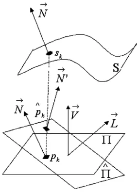
[image:4.594.355.496.65.263.2]We work on a plane perpendicular to the light source di-rection. Let be the coordinates of the point with pixel index on the plane . Since the surface normals is con-strained to fall on the irradiance cone and we are working on
Fig. 1. Geometry of the SFS process.
the plane perpendicular to the light source direction, the com-ponent of the surface normal is equal to the normalized image brightness .
In this paper, our idea is to recover the azimuthal compo-nent using a heat-equation smoothing process. To do this we introduce a scalar field on the rotated image plane . The az-imuthal component of the surface normal is the gradient of this scalar field. The scalar field is assumed to be subject to the heat equation, and the associated heat flow or diffusion process is responsible for smoothing the azimuthal component of the sur-face normal. Although the azimuthal component of the sursur-face normal is determined by the gradient of the scalar field, in prac-tice we are only interested in the polar angle of the gradient vector since this determines the azimuthal angle of the surface normal. The heat equation provides a means of smoothing the azimuthal directions of the surface normals on the plane .
To be more formal, let be a time-dependent field on the plane , where is the coordinate vector of the point and is the time epoch. According to Fourier’s law, the heat flow vector is related to the gradient of the scalar potential field through the expression
(5)
The magnitude of the time derivative of the heat flow is related to the time derivative of the scalar potential via the heat diffusion equation
(6)
where and are proportionality constants. With these ingre-dients, the azimuthal angle of the surface normal on the plane can then be found by computing the angle between the com-ponents of the gradient for the scalar field , which is given by
10 IEEE TRANSACTIONS ON IMAGE PROCESSING, VOL. 16, NO. 1, JANUARY 2007
Fig. 2. Top row, from left to right: Ground truth height data, rendering of the test shape using Lambert’s law with added noise, field of surface normals at the first and final iterations of the algorithm. Bottom row, from left to right: Heat functionQ(x; y; t)fort = 1,t = 3,t = 6, andt = 9.
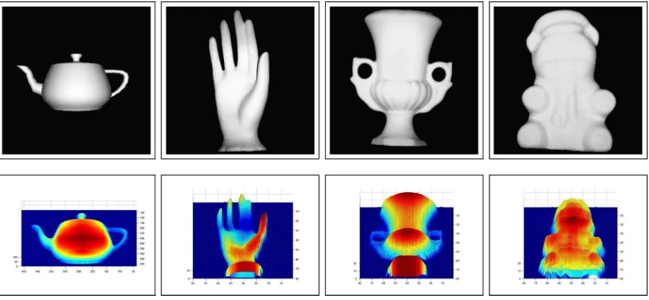
Fig. 3. Shape-from-shading results on real-world data. Top row: Input images whose specularities have been removed. Bottom row: Ground truth depth data.
brightness at the point . Hence, and by expanding the Laplacian, we can rewrite the heat diffusion equation as fol-lows:
(7) To take our analysis further, we rely on the phys-ical meaning of the right-hand side of (7). The quan-tity is the rate of energy increase for an element of surface enclosed by a region . Hence, we can normalize the heat-flow to unity by setting . As a result, and after rearranging terms, we get
(8)
and, therefore, we have
(9)
where we have set .
At this point, since we are working on a uniformly sampled pixel lattice, we can consider uniform regions of area across the plane and rewrite the equation above as follows:
(10)
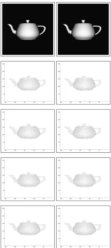
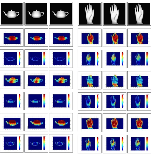
[image:5.594.64.532.311.528.2]func-Fig. 4. First row: Input images with noise added. Second and third rows: Field of surface normals delivered by the algorithm of Worthington and Hancock after ten and 100 iterations. Fourth and fifth rows: Field of surface normals at the initial and final iterations of our method.
tion . We commence by setting . At time step , the update equation for the point indexed is
[image:6.594.45.282.62.590.2](11) where is the set of points adjacent to . The quantity is the averaged and normalized scalar potential, computed using
Fig. 5. First row: Input images with noise added. Second and third rows: Field of surface normals delivered by the algorithm of Worthington and Hancock after ten and 100 iterations. Fourth and fifth rows: Field of surface normals at the initial and final iterations of our method.
the formula
(12)
[image:6.594.307.545.66.589.2]12 IEEE TRANSACTIONS ON IMAGE PROCESSING, VOL. 16, NO. 1, JANUARY 2007
Fig. 6. First row: Input images with noise added. Second and third rows: Field of surface normals delivered by the algorithm of Worthington and Hancock after ten and 100 iterations. Fourth and fifth rows: Field of surface normals at the initial and final iterations of our method.
at the location indexed is given by
(13)
In the above equation, and
are the first difference approximations to the and
compo-Fig. 7. First row: Input images with noise added. Second and third rows: Field of surface normals delivered by the algorithm of Worthington and Hancock after ten and 100 iterations. Fourth and fifth rows: Field of surface normals at the initial and final iterations of our method.
nents of the gradient of , and are given by
(14)
[image:7.594.304.546.61.593.2]Fig. 8. Error as a function of variance for the four objects in our dataset.
sign of the flow in the and directions on the plane to determine the sign of surface normal components. Thus, in the rotated frame of reference the surface normal is given by
where . With the surface normal in the rotated frame of reference at hand, the surface normal on the image plane may be computed making use of the rotation matrix
as given in (4).
IV. SURFACEHEIGHTRECOVERY
In this section, we address the problem of recovering the sur-face height function from the pattern of local height differences. To do this, we use the field of surface normals to estimate the height difference between each pair of pixel sites in the image. Once the height estimates have been computed, the surface may be then recovered by embedding them into the unidimensional Euclidean space perpendicular to the lattice footprint.
A. Height Difference Approximation
Let be the estimate of the surface height difference be-tween the pair of points and on the surface under study whose and coordinates correspond to the row and column indexes of the pixels and on the image plane. An esti-mate of may be recovered by making use of the incre-ments along the pixel-sites falling on the path that best describes the projection of the geodesic connecting the points on the surface onto the image or pixel lattice. To compute the quan-tity , we traverse the path and compute the height increments associated with the pixel-site transitions along the path. The quantity is then given by the sum of these height increments. The approximation to the height increment associ-ated with the transition from the pixel indexed to the pixel indexed can be computed by assuming that the two pixel sites are connected by a line whose slope is determined by the normal vectors and . The height increment is given by
(15)
14 IEEE TRANSACTIONS ON IMAGE PROCESSING, VOL. 16, NO. 1, JANUARY 2007
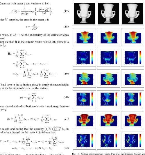
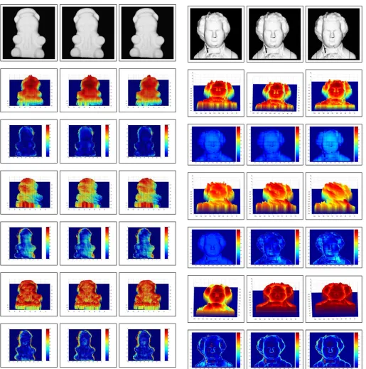
Fig. 9. Surface height recovery results. First row: Input images. Second and third rows: Recovered height and mean-squared error for our method. Fourth and fifth rows: Recovered height and mean-squared error for the method of Frankot and Chellappa. Sixth and seventh rows: Recovered height and mean-squared error for the method of Horn and Brooks.
B. Surface Integration via Unidimensional Embedding
The problem of recovering the surface from a set of pairwise height difference estimates may be viewed as one of unidimen-sional embedding subject to constraints provided by the foot-print of the image lattice. We commence by rewriting the height difference estimate between a pair of points on the sur-face as
(16)
Fig. 10. Surface height recovery results. First row: input images. Second and third rows: Recovered height and mean-squared error for our method. Fourth and fifth rows: Recovered height and mean-squared error for the method of Frankot and Chellappa. Sixth and seventh rows: Recovered height and mean-squared error for the method of Horn and Brooks.
where is the surface height at a point corresponding to the pixel-site indexed and is the error of representation in the height difference.
be Gaussian with mean and variance , i.e.,
(17)
For the samples, the error in the mean is
(18)
As a result, as , the uncertainty of the estimator tends to zero.
Suppose that is the column-vector whose th element is given by
(19)
The final term in the definition above is simply the mean height error at the location indexed on the surface
(20)
If we assume that the distribution of errors is stationary, then we can write
(21)
As a result, and noting that the quantity in (19) does not depend on the index , it follows that:
(22)
Finally, if we set and solve for . The result is
(23)
It is important to stress that, whereas setting may alter the position of the surface with respect to the coordinate system, the relative height configuration of each pair of points remains unchanged.
C. Approximation by Subsampling
[image:10.594.53.552.60.591.2]The complexity of performing the embedding depends on the image dimension . This may become burdensome for large images. To overcome this problem, for large images, we can
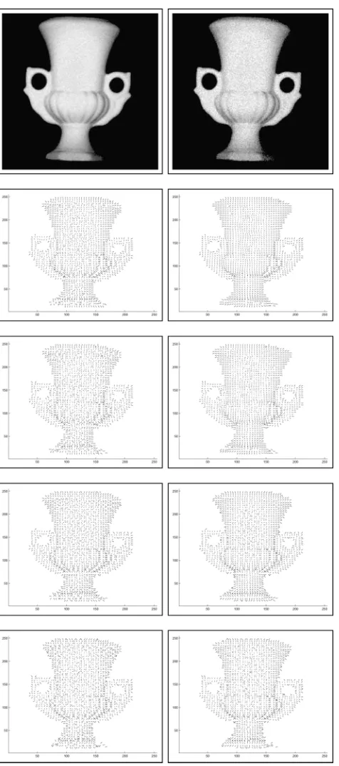
Fig. 11. Surface height recovery results. First row: input images. Second and third rows: Recovered height and mean-squared error for our method. Fourth and fifth rows: Recovered height and mean-squared error for the method of Frankot and Chellappa. Sixth and seventh rows: Recovered height and mean-squared error for the method of Horn and Brooks.
make use of the central limit theorem [23] to develop an accurate subsampling method. To do this, we commence by defining the
th coefficient of the vector as follows:
16 IEEE TRANSACTIONS ON IMAGE PROCESSING, VOL. 16, NO. 1, JANUARY 2007
Fig. 12. Surface height recovery results. First row: Input images. Second and third rows: Recovered height and mean-squared error for our method. Fourth and fifth rows: Recovered height and mean-squared error for the method of Frankot and Chellappa. Sixth and seventh rows: Recovered height and mean-squared error for the method of Horn and Brooks.
where is the subset of sample pixel-sites used for computing the height difference estimates for each of the coefficients . Since the length of the vectors and is the same, the reso-lution of the surface remains unchanged. If the probability dis-tribution for is Gaussian with variance , then the surface height can be reconstructed using the formula
(25)
Fig. 13. Surface height recovery results. First row: input images. Second and third rows: Recovered height and mean-squared error for our method. Fourth and fifth rows: Recovered height and mean-squared error for the method of Frankot and Chellappa. Sixth and seventh rows: Recovered height and mean-squared error for the method of Horn and Brooks.
The precision of the estimate is
(26)
Fig. 14. Surface height recovery results. First column: Input images. Second column: Height recovered using our method. Third column: Recovered height for the method of Frankot and Chellappa. Fourth column: Recovered height for the method of Horn and Brooks.
V. EXPERIMENTS
In this section, we provide experiments with our new shape-from-shading method. The experimental study is divided into two parts. We commence by focussing on the performance of the heat-equation method for surface normal recovery. In the second part, we concentrate on the process of surface height recovery. The experimental study involves both, synthetic and real-world data.
A. Surface Normal Recovery
We commence our experimental study by illustrating the utility of the heat-equation method for recovering smoothed fields is surface normals. Here, we have experimented with images which exhibit significant levels of noise. To this end, we have added controlled levels of Gaussian noise to synthetic and real-world imagery of objects that exhibit Lambertian reflectance. In all our experiments, we follow Worthington and Hancock [12] and use the grayscale gradient as an initial estimate of the surface normal field directions.
In Fig. 2, we illustrate the behavior of the method on synthetic data. Here the left-most panel in the top row shows the syn-thetic surface used in our study. This consists of two parabolic domes superimposed on a parabolic ridge. The second panel
in the top row shows the result of rendering the surface using Lambert’s law. The third and fourth panels in the top row show the initial and final fields of surface normals delivered by the method. Initially, the field of surface normals is relatively disor-ganized, and appears noisy. The main effect to note here is that the heat-kernel smoothing method rotates the surface normal so that a consistent field emerges that reflects well the geometry of the underlying surface. In the bottom row of the figure, we show the heat function as a function of time . Each plot displays the value of as a height value on the plane for fixed values of , i.e., 1, 3, 6, 9. Here, con-vergence is reached after nine iterations. Therefore, in Fig. 2, we have chosen the values of so as to be uniformly distributed from to . The main elevation features of the surface emerge as peaks in the plots of , and, as time evolves, they become sharpened.
18 IEEE TRANSACTIONS ON IMAGE PROCESSING, VOL. 16, NO. 1, JANUARY 2007
Fig. 15. Surface height error as a function of the variance for the objects in our dataset.
bottom line of the figure we show the ground truth data used in our study. This consists of depth images of the objects studied, captured using a Polhemus structured light range-sensor. The range data have been aligned with digital images using a simple registration algorithm.
In Figs. 4–7, we show the surface normal results obtained from the digital images. The top row of each figure shows noise corrupted versions of the input images. Here, we have added
normals that are both smoother and contain more fine surface detail than that of Worthington and Hancock. For instance, the surface structure of the hand, the ribs of the urn and the limbs of the bear all emerge more clearly when our method is used.
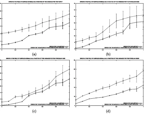
A more quantitative analysis of the results is shown in Fig. 8. Here, we show plots of the mean-squared error in the recon-structed surface normal directions as a function of the variance of the added Gaussian noise. For each object, we have com-puted the mean square error between the surface normal direc-tions delivered by shape-from-shading method and those com-puted from the aligned ground truth range images. Fig. 8(a) is for the teapot, Fig. 8(b) is for the hand, Fig. 8(c) is for the urn, and Fig. 8(d) for the model bear. In each plot, the solid curve is the result of applying our method and the dotted curve that of applying the Worthington and Hancock method. The error bars show the standard error in the mean-squared errors. The features to note from the plots are as follows. First, the mean-squared error grows approximately linearly with the noise variance. Second, our new method gives errors which are consis-tently lower than those delivered by the Worthington and Han-cock method.
B. Surface Height Recovery
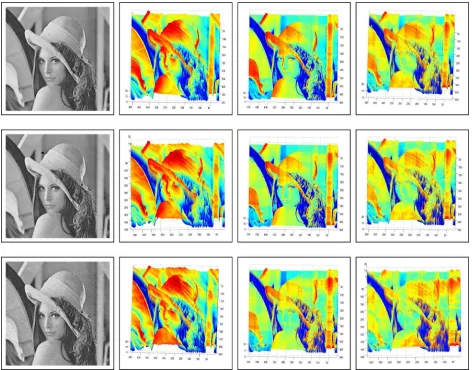
Having examined the behavior of the heat-flow method for vector field smoothing, in this section we turn our attention to the effectiveness of our method for surface height recovery. We commence with experiments on synthetic data which are aimed at evaluating the systematics and noise sensitivity of the method, and then provide some experiments on real world data. We also present results on the “Mozart” and the “Lena” images. We have done this so as to provide the reader with results that can be used for the purposes of comparison with other work presented elsewhere in the literature. In all of our experiments, we have set so as to achieve a precision .
In Figs. 9–13, we investigate the effect of added image noise on the reconstructed height. In the top row of the figures, from left to right, we show the input images with zero added noise, and with added noise with zero mean and a standard devia-tion of 0.3 and 0.5 grey levels. In the second and third rows of each figure, we show the reconstructed height and the differ-ence between the ground truth and reconstructed height using our method. In the fourth and fifth rows we show the corre-sponding results obtained using the Frankot and Chellappa [21] method, and the sixth and seventh rows those obtained using the Horn and Brooks [10] method. The main features to note from these plots are as follows. First, our method gives good reconstruction of the surface detail even under the highest level of noise. Second, the errors obtained with our method are con-fined to the boudaries of the objects, and the locations of sharp surface cusps. Third, the Horn and Brooks method recovers sur-faces that show significant error over the entire object.
[image:14.594.304.551.66.580.2]We show the results for the image of “Lena” in Fig. 14. Un-fortunately, mean-squared error measures could not be provided since there is no ground truth available for this image. Nonethe-less, we have investigated the effect of added image noise on the reconstructed height by adding noise with zero mean and known standard deviation. In the figure, the top row shows the results for the noise-free image. The second and third rows show the
Fig. 16. Surface height recovery results. First row: Input images. Second and third rows: Recovered height and mean-squared error for our method. Fourth and fifth rows: Recovered height and mean-squared error for the method of Frankot and Chellappa. Sixth and seventh rows: Recovered height and mean-squared error for the method of Horn and Brooks.
results for the noise-added imagery with standard deviation of 0.3 and 0.5, respectively. For each row, we show, from left to right, the input image, the recovered height for our algorithm and the depth maps for the algorithms of Frankot and Chellapa [21] and Horn and Brooks [10].
20 IEEE TRANSACTIONS ON IMAGE PROCESSING, VOL. 16, NO. 1, JANUARY 2007
Fig. 17. Surface height error as a function of the angle between the light source and the viewer directions for the teapot.
TABLE I
PROCESSINGTIMES FOR THESURFACEHEIGHTRECOVERYPROCESS
the Frankot and Chellappa’s method, and the solid curve is that obtained using the Horn and Brooks method. The height errors obtained using our method are consistently lower than those ob-tained with the two alternatives. It is interesting to note that the slope of the curves are very close, but that the error at zero noise is smallest for our method. This means that even when there is no added noise, the alternative methods result in significant surface reconstruction error. In other words they exhibit bias.
Next, we turn our attention to the effects of variation in light source direction. For this study we use the teapot. To this end, we have generated a set of six images illuminated with a single light source positioned in the direction . For our experiments, we have set and varied the angle . Inorder to avoid self-shadowingeffects, we have limited our attention to the values of the angle between 0 and 50 .
In the top row of Fig. 16, we show three of the images in our dataset. Here, we have ordered the example images, from left to right, in increasing , i.e., 0 , 20 , 50 . The second and third rows in the figure show, again, the recovered height and, the difference between the recovered and the ground-truth heights. The results for the methods of Horn and Brooks and Frankot and Chellappa are shown in the bottom rows. The errors are largest at highly inclined locations on the surface. Whereas the effect of varying the light source direction is to magnify the errors for both methods, our algorithm is more robust and de-livers better results. Fig. 17 provides a quantitative investiga-tion of this effect. Here we plot the mean-squared height error for the three methods as a function of the angle between viewer and light source directions. In the left-hand panel, we show the mean-squared error when our heat flux method is used to recover the surface normal directions. The right-hand panel shows the error plots when the Worthington and Hancock method is used.
Again, the error for the alternatives is consistently larger than the one given by our method.
Finally, we present timing statistics for our method and the other two alternatives. All our experiments were performed on a Pentium 4, 3-GHz PC. It is worth noting that the imple-mentations of our method and those of Horn and Brooks and Frankot and Chellappa are not fully optimized, and, hence, the timings shown below are provided as an illustration of the algorithms performance. The method of Horn and Brooks [10] hinges around solving a Poisson equation subject to the natural boundary condition. In this case, a solver based on the finite element method was used. In the method developed by Frankot and Chellappa [21], integrability is enforced making use of an optimisation process in the Fourier domain. Here, we have used a fast Fourier transform (FFT).
In Table I, we show the processing times for the results pre-sented in Fig. 15. In the table, we show the mean and variance for the height recovery timings when processing the imagery with different levels of added noise. From the table, it is clear that the algorithm of Horn and Brooks is the one whose computa-tional complexity is largest. This is due to the differential equa-tion solver invoked by the method at runtime. Our algorithm is slightly more computationally intensive than the algorithm of Frankot and Chellappa, but much more efficient than the one of Horn and Brooks.
VI. CONCLUSION
posed the problem of recovering the surface height as a that of embedding the field of surface normals into a manifold that resides in a Euclidean space. We have also shown how the complexity of the embedding process may be greatly reduced by a subsampling approach. We have performed experiments on synthetic and real-world imagery.
There are a number of ways in which the work reported in this paper may be further extended. First, we aim to explore how constraints from differential geometry can be incorporated into the heat-flow smoothing process. This is a problem that has been extensively studied in the context of Beltrami flows [25] and may allow us to incorporate information concerning surface topography. Second, we aim to explore more deeply the relationship between the scalar potential and the structure of the underlying surface. For instance, it would be interesting to explore the relationship between the divergence of the scalar potential and the surface curvature.
REFERENCES
[1] E. Mingolla and J. Todd, “Perception of solid shape from shading,”
Biol. Cybern., vol. 53, pp. 137–151, 1986.
[2] P. N. Belhumeur and D. J. Kriegman, “What is the set of images of an object under all possible lighting conditions?,”Comput. Vis. Pattern Recognit., pp. 270–277, 1996.
[3] M. Bichsel and A. P. Pentland, “A simple algorithm for shape from shading,” inProc. IEEE Conf. Computer Vision and Pattern Recogni-tion, 1992, pp. 459–465.
[4] R. Kimmel, K. Siddiqqi, B. B. Kimia, and A. M. Bruckstein, “Shape from shading: Level set propagation and viscosity solutions,”Int. J. Comput. Vis., vol. 16, pp. 107–133, 1995.
[5] A. M. Bruckstein, “On shape from shading,”Comput. Vis., Graph., Image Process., vol. 44, no. 2, pp. 139–154, 1988.
[6] P. Dupuis and J. Oliensis, “Direct method for reconstructing shape from shading,” in Proc. IEEE Conf. Computer Vision and Pattern Recognition, 1992, pp. 453–458.
[7] A. Robles-Kelly and E. R. Hancock, “A graph-spectral approach to shape-from-shading,”IEEE Trans. Image Process., vol. 13, no. 7, pp. 912–926, Jul. 2004.
[8] R. Zhang, P. S. Tsai, J. E. Cryer, and M. Shah, “Shape from shading: A survery,”IEEE Trans. Pattern Anal. Mach. Intell., vol. 21, no. 8, pp. 690–706, Aug. 1999.
[9] K. Ikeuchi and B. K. P. Horn, “Numerical shape from shading and oc-cluding boundaries,”Artif. Intell., vol. 17, no. 1–3, pp. 141–184, 1981. [10] B. K. P. Horn and M. J. Brooks, “The variational approach to shape
from shading,”CVGIP, vol. 33, no. 2, pp. 174–208, 1986.
[11] Q. Zheng and R. Chellappa, “Estimation of illuminant direction, albedo, and shape from shading,”IEEE Trans. Pattern Anal. Mach. Intell., vol. 13, no. 7, pp. 680–702, Jul. 1991.
[12] P. L. Worthington and E. R. Hancock, “New constraints on data-close-ness and needle map consistency for shape-from-shading,”IEEE Trans. Pattern Anal. Mach. Intell., vol. 21, no. 12, pp. 1250–1267, Dec. 1999. [13] S. Osher and J. Sethian, “Fronts propagating with curvature-dependent speed: Algorithms based on hamilton,”J. Comput. Phys., vol. 79, pp. 12–49, 1988.
[14] J. D. Durou and H. Maitre, “On convergence in the methods of strat and of smith for shape from shading,”Int. J. Comput. Vis., vol. 17, no. 3, pp. 273–289, 1996.
[15] E. Rouy and A. Tourin, “A viscosity solution approach to shape-from-shading,”SIAM J. Numer. Anal., vol. 29, no. 3, pp. 867–884, 1992. [16] E. Prados and O. Faugeras, “Perspective shape from shading and
vis-cosity solutions,” inProc. IEEE Int. Conf. Conputer Vision, 2003, pp. II:826–831.
[17] R. Kimmel and A. M. Bruckstein, “Tracking level sets by level sets: A method for solving the shape from shading problem,”Comput. Vis. Image Understand., vol. 62, no. 2, pp. 47–48, Jul. 1995.
[18] R. Kimmel, R. Malladi, and N. Sochen, “Images as embedded maps and minimal surfaces: Movies, color, texture, and volumetric medical images,”Int. J. Comput. Vis., vol. 39, no. 2, pp. 111–129, 2000.
[19] B. K. P. Horn, “Height and gradient from shading,”Int. J. Comput. Vis., vol. 5, no. 1, pp. 37–75, 1990.
[20] Z. Wu and L. Li, “A line-integration based method for depth recovery from surface normals,”CVGIP, vol. 43, no. 1, pp. 53–66, Jul. 1988. [21] R. T. Frankot and R. Chellappa, “A method of enforcing integrability
in shape from shading algorithms,”IEEE Trans. Pattern Anal. Mach. Intell., vol. 4, no. 10, pp. 439–451, Oct. 1988.
[22] T. Wei and R. Klette, “Theoretical analysis of finite difference algo-rithms for linear shape from shading,”CAIP, pp. 638–645, 2001. [23] A. Papoulis, Probability, Random Variables, and Stochastic
Pro-cesses. New York: Mc Graw-Hill, 1984.
[24] A. Robles-Kelly and E. R. Hancock, “Estimating the surface radiance function from single images,”Graph. Models, to be published. [25] N. Sochen, “Affine invariant flows via the beltrami framework,”J.
Math. Imag. Vis., vol. 20, pp. 133–145, 2004.
Antonio Robles-Kelly(M’96) received the B.Eng. degree in electronics and telecommunications from the Instituto Tecnologico y de Estudios Superiores de Monterrey, Monterrey, Mexico (with honors) in 1998, and the Ph.D. degree in computer science from the University of York, York, U.K., in 2003.
In 2001, as a graduate student at the University of York, he visited the University of South Florida as part of the William Gibbs/Plessey Award for the best research proposal to visit an overseas research lab-oratory. After receiving his doctorate, he was a Re-search Associate under the MathFit-EPSRC framework at the University of York until December 2004. Currently, he is a Research Scientist with National ICT Australia, Australian National University, Canberra Laboratory, Canberra, where he leads the Spectral Imaging and Source Mapping (SISM) project of the Vision Systems, Technologies, and Applications (ViSTA) programme. His research interests are in the areas of computer vision, pattern recognition, and computer graphics. Along these lines, he has done work on segmentation and grouping, graph matching, shape-from-X, hyperspectral image understanding, and relectance models. He is also interested in the diffrential structure of sur-faces.
Edwin Hancockreceived the degree in physics and the Ph.D. degree in high-energy physics from the University of Durham, Durham, U.K., in 1977 and 1981, respectively.
For ten years, he was a Researcher in the fields of high-energy nuclear physics and pattern recog-nition at the Rutherford-Appleton Laboratory (now the Central Research Laboratory of the Research Councils), Cheshire, U.K. During this period, he also held adjunct teaching posts at the University of Surrey, Surrey, U.K., and the Open University, Milton Keynes, U.K. In 1991, he joined the University of York, York, U.K., as a Lecturer in the Department of Computer Science. He was promoted to Senior Lecturer in 1997 and to Reader in 1998. In 1998, he was appointed to a Chair in Computer Vision. He now leads a group of some 15 faculty, research staff, and Ph.D. students working in the areas of computer vision and pattern recognition. He has been a Guest Editor for special issues of the journalsImage and Vision ComputingandPattern Recognition. He has been a member of the Editorial Board forPattern Recognition. He has published over 80 journal papers and 300 refereed conference publications. He has been on the program committees for numerous national and international meetings. In 1997, with Marcello Pelillo, he established a new series of international meetings on energy minimization methods in computer vision and pattern recognition. His main research interests are in the use of optimization and probabilistic methods for high- and intermediate-level vision. He is also interested in the methodology of structural and statistical pattern recognition. He is currently working on graph matching, shape-from-X, image databases, and statistical learning theory. His work has found applications in areas such as radar terrain analysis, seismic section analysis, remote sensing, and medical imaging.