Article
Dynamic Response of 2 Piles in Series and Parallel
Arrangement
Kiran B. Ladhane
aand Vishwas A. Sawant
b,*
Department of Civil Engineering, Indian Institute of Technology, Roorkee, Uttarakhand 247667, India Email: [email protected], [email protected]b,*
Abstract. In the present study, dynamic analysis of laterally loaded vertical pile group is carried out considering the three dimensional nature of the soil-pile system. Piles and soil are modelled using three-dimensional finite element techniques treating them as linear elastic. The interface of soil and pile under the lateral load has been accounted for by incorporating interface elements in the modelling. The special type of transmitting boundary using Kelvin element is used to transfer the propagating waves from near field to the far field. Group of two piles in series and parallel configuration have been considered for present study. Individual piles are considered monolithic with pile cap. Parametric studies have been performed to examine the effects of pile spacing and soil modulus on the response of pile group.
Keywords: 3D finite element analysis, dynamic analysis, Kelvin element, transmitting boundary.
ENGINEERING JOURNAL Volume 16 Issue 4 Received 12 March 2012
Accepted 22 April 2012 Published 1 July 2012
1.
Introduction
The behaviour of piles subjected to dynamic loads is a complex three-dimensional soil–structure interaction problem mainly governed by the interaction between the pile and the soil. Several analytical methods have been developed in the past for static analysis of laterally loaded piles, including the elastic continuum approach [1, 2], finite element analysis [3], elastic subgrade reaction [4, 5, 6], and p–y [7, 8] methods.
Novak (1974) [9] was first to extend a Winkler model for the representation of soil in dynamic analysis of laterally loaded pile in a visco-elastic material. Ghazzaly et al. (1976) [10] presented a rational approach in which the pile response is represented by the vibrations of a beam on elastic foundation. Finite difference technique is used to solve the governing fourth order differential equation. The semi-analytical solution of the dynamic behavior of vertical pile group is presented by Ettouney et al. (1983) [11]. The solution accounts for the pile-soil-pile dynamic interaction and is based on modeling the soil as a plane strain continuum and the piles as a set of finite elements. Gazetas (1984) [12] presented a numerical study of the dynamic response of end-bearing piles embedded in a number of idealized soil deposits and subjected to vertically propagating harmonic S-waves.
Adopting Winkler assumption, a simple mechanical soil model is developed for the flexural response analysis of dynamically loaded single pile by Nogami and Konagai (1988) [13]. Nogami et al. (1992) [14] developed a hybrid near field/far field soil-pile interaction models for dynamic loading and formulated solutions for axial and lateral response in the time and frequency domains, incorporating nonlinear soil-pile response, degradation, gapping, slip, radiation damping, and loading rate effects. Gazetas et al. (1993) [15] presented seismic soil-pile-foundation structure interaction analysis based on Beam-on-Dynamic-Winkler-Foundation (BDWF) simplified model and a Green's-function-based rigorous method are utilized in determining the dynamic response of single piles and pile groups.
Naggar and Novak (1995) [16] presented a model for pile lateral response to transient dynamic loading and to harmonic loading allowing for nonlinear soil behavior, discontinuity condition at the pile-soil interface and energy dissipation through different types of damping. The approach is based on the Winkler hypothesis. Badoni and Makris (1996) [17] given the macroscopic model that consists of distributed hysteretic springs and frequency dependent dashpots to model the lateral soil reaction and a practical method based on one-dimensional finite element formulation is developed to compute the nonlinear response of single piles under dynamic lateral loads.
Nogami and Novak (1976) [18] studied the interaction between a soil layer and bearing pile in vertical vibration. The pile was assumed to be elastic, vertical and bearing while the soil as linearly elastic, homogenous and isotropic layer with material damping of the frequency independent hysteric type and overlies rigid bed rock. Novak and Nogami (1977) [19] extended the same concept to investigate the resistance of a soil layer to steady horizontal vibration of an elastic end bearing pile. Further Chau and Yang (2005) [20] extended it to incorporate the effect of nonlinear soil–pile interaction subject to horizontal shaking of a vertical circular pile embedded in a soil layer of finite thickness.
Cai et al. (2000) [21] investigated more precisely the seismic response of interactive soil–pile– structure systems; a three-dimensional finite element subsystem methodology with an advanced plasticity-based constitutive model for soils has been developed. Maheshwari and Emani (2008) [22] and Emani and Maheshwari (2009) [23] presented the dynamic impedances for the pile groups with caps embedded in isotropic homogeneous elastic soils. A general three-dimensional finite element procedure is developed. The system is sub-structured into bounded near-field and an unbounded far-field. The pile-soil system of the near-field is modeled using solid finite elements, and the unbounded elastic soil system of the far-field is modeled using the consistent infinitesimal finite element cell method (CIFECM) in the frequency domain. Maheshwari and Emani (2008) [22] further carried out non linear seismic analysis of 2 X 2 pile group. A work-hardening plastic cap model was used for constitutive modeling of the soil medium. The pore pressure generation for liquefaction was incorporated by a two-parameter volume change model.
2.
Problem Definition
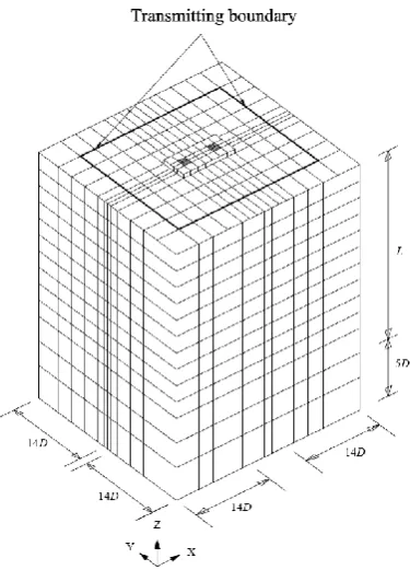
in Fig. 1(b), when direction of loading is parallel to the line joining piles; it is considered as series arrangement. In parallel arrangement direction of loading is perpendicular to the line joining piles. Three dimensional finite element methods are used to model the soil-pile system. The supporting soil medium domain is divided into two regions as near field and far field. The near field is within the range of 10D (D is width of pile)from the edge of exterior pile along the width of domain on all sides of pile group. The near field boundary is modelled as transmitting boundary. To the exterior boundary nodes of the near field Kelvin Elements are attached in both the directions which are supposed to absorb the energy waves propagating in horizontal and vertical directions and thus not allowing them to reflect back into the near field. Beyond this, the soil domain represents the far field (4D from transmitting boundary. The Pile and soil are treated as linear elastic. The soil considered in present study is medium clay which is partially saturated due to capillary action. Figure 1 shows the details of soil pile system considered for present study.
Fig. 1(a). Typical view of soil pile system for 2 piles. Fig. 1(b). Arrangement of piles in group.
[image:3.595.108.255.225.365.2] [image:3.595.205.393.409.670.2]3.
Methodology of Research
3.1. Finite Element Model for Analysis of Laterally Loaded Piles
A program is developed in FORTRAN which is capable of carrying out full three dimensional finite element analysis incorporating transmitting boundary. Full three-dimensional geometric model is used to represent the soil-pile system. Selection of the correct finite element to represent the medium is one of the very important aspect in finite element analysis. In the soil pile system two materials viz. soil and reinforced concrete are to be modelled. Both the materials show the different behaviours when subjected to loading. The failure of soil is dominated by its shear characteristics; whereas flexure dominated failure is shown by the reinforced concrete. Therefore, to model the pile and pile cap 20 node solid finite elements are used. This element has quadratic shape function which is well suited to model the medium with bending dominated deformation. Eight node solid finite elements are used to model the soil which has linear shape functions. These elements are suitable for the medium whose deformations are dominated by shear strength. To maintain the continuity of displacement between these two types of the elements in the discretised pile-soil domain, two more elements were formulated viz. 12 node and 9 node solid elements. The shape functions of these two elements were formulated by degrading the shape functions of 20 node solid elements. 12 node elements are used at the junction where 8 node and 20 node element meets. 9 node elements are used at the junction of 8 node element and 12 node element. The shape functions of these elements are derived by degrading the 20 node element. Each node of the elements has three translational degrees of freedom, in the X, Y and Z coordinate directions. The interface between pile or pile cap and soil is modeled using 16 node isoparametric interface elements with zero thickness [24]. These interface elements are useful in simulating the mechanics of stress transfer along the interface of soil and pile. Piles and soil are treated as linear elastic. A 20m long square piles of side 1m are considered for present study. The piles are completely embedded in the soil.
3.2. Continuum Element
Relation between strains and nodal displacements is expressed as,
e
B e (1)where {ε}e is strain vector, {δ}e is vector of nodal displacements, and [B] is strain displacement transformation matrix. The stress-strain relation is given by,
e
D e (2)where, {σ}e is stress vector, and [D] is constitutive relation matrix. The stiffness matrix of an element is expressed as,
T
e V
K
B D B dv (3)3.3. Interface Element
Relative displacements (strains) between the surface of soil and structure induce stresses in the interface element. These relative displacements are given as,
e
B f
e (4)where, [B]f represents the strain displacement transformation matrix. The element stiffness is obtained by the usual expression,
Te f f f
S
K
B D B ds (5)where, [D]f is the constitutive relation matrix for the interface.
3.4. Equivalent Nodal Force Vector
The lateral force FH, acting on pile cap, is considered as uniformly distributed force over the pile cap. The
T e
A
Q
q N dA (6)where [N] represents matrix of shape functions. The properties of materials used in present study are shown in the Table 1.
Table 1. Properties of materials.
Pile Soil Interface
Ep =25 GPa
νp= 0.30
Width 1 m, Length 20 m Pile-cap thickness 0.5 m
Es =10000 kPa, 20000 kPa, 30000 kPa, 40000 kPa
νs = 0.40
ks=1000 kN/m3
kn=1.0×10⁶ kN/m3
Ep and Es = Modulus of elasticity for pile and soil respectively, νp and νs = Poisson's ratio for pile and soil respectively, ks and kn = Tangential and normal stiffness for interface element.
3.5. Transmitting Boundary
The spring and dashpot constants of the Kelvin element in the horizontal directions are calculated using the solution developed by Novak (1974) [9] as:
1 2
*
2 R S iS G
k o
r (7)
In which, G is the shear modulus of soil, kr* is the complex stiffness and, Ro is the radial distance of the
node where the Kelvin element is attached from the source of vibration. S1 and S2=dimensionless
parameters from closed-form solutions, i=imaginary unit= 1. The real part of the above Eq. (7)
represents the stiffness and the imaginary part represents the damping. The constants for the Kelvin element in vertical direction are given by
1 2
*
2 o v v
v S iS
R G
k
(8)
The subscript v represents the vertical direction and the other parameters are the same as in Eq. (7).
3.6. Time History Analysis
Dynamic force equilibrium equation in incremental form
M
qi
C
qi
K
qi Fi (9)In which
qi , qi , qi are vectors of incremental displacement, velocity and acceleration, [K]assembled stiffness matrix, [M] consistent mass matrix and [C] damping matrix.
The displacement at each time step can be evaluated by applying Newmark-Beta integration method. After application of Newmark-Beta integration method, Dynamic force equilibrium equation in incremental form is given as follows.
1 2 1 1 1 1 1 2 2i i i
i
M C K q F M C q
t t
t
M t C q
(10)
The values of and in above equation are taken as 0.5 and 0.25 respectively. Solution of the above equation yields incremental displacement
qi from which displacements at current time step areupdated and Velocity and accelerations are evaluated. For next time step the values of
qi1
, qi1
, qi1
are set as
qi , qi , qi and analysis is performed for next dynamic load4.
Parametric Study
A parametric study is carried out on the group of two piles in series and parallel configuration. The dynamic load of the type P0sin(ωt) (P0=1000 kN for present case) is applied, where the external frequency (ω) is varied between 0.5 to 40 rad/sec. All piles considered in the analysis are square concrete piles. In present study L/D ratio is considered as 20 and spacing to width (s/D) ratio between piles is varied as 2, 3, 4, 5 and 7 (D is width of square pile). Top displacements in the pile considered for comparison of different responses.
5.
Results and Discussion
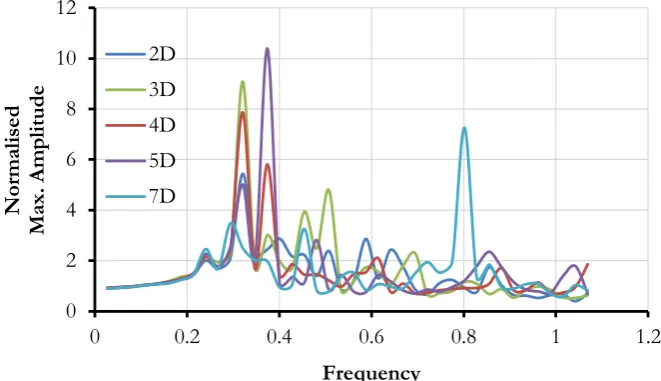
The response of pile group is presented in the form of normalized maximum amplitude verses dimensionless frequency. The maximum amplitudes obtained are normalized by dividing them with corresponding static deflection. The dimensionless frequency a0 is calculated using a0 = d/Vs (where, is forcing frequency in rad/sec, d is width of square pile and Vs is shear wave velocity). The variations in normalized maximum amplitude with dimensionless frequency at different pile spacing for piles in series and parallel arrangement (Es=20000 kPa) is presented in Figs. 2 and 3, respectively.
Fig. 2. Frequency-Amplitude Curve for two pile in series arrangement and Es=20000 kPa.
0 2 4 6 8 10 12 14
0 0.1 0.2 0.3 0.4 0.5 0.6 0.7 0.8
N
or
m
alise
d
Ma
x.
A
m
plit
ud
e
Dimensionless Frequency, a0
2D 3D 4D 5D 7D
0 2 4 6 8 10 12
0 0.2 0.4 0.6 0.8 1 1.2
N
orm
al
ise
d
M
ax
. Am
pl
it
ud
e
Frequency
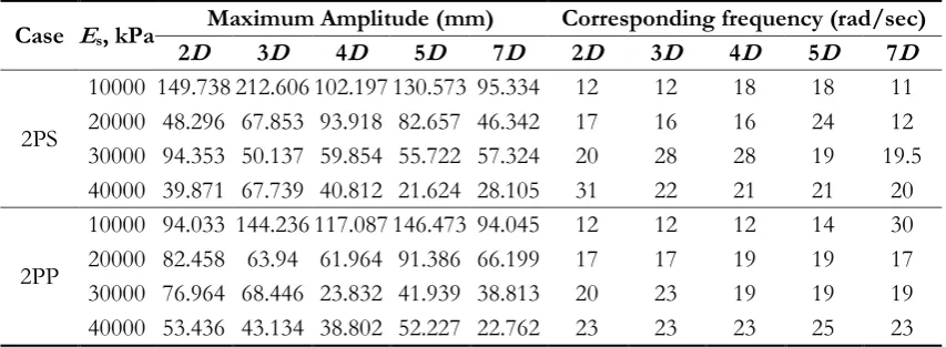
[image:6.595.132.476.302.498.2] [image:6.595.133.464.555.745.2]When the external frequency is matching with natural frequency of the system, a clear peak in the response is observed. The frequencies corresponding to first three prominent peaks are summarized in Table 2. In case of series arrangement, the fundamental frequency corresponding to first peak at the pile spacing of 2D is observed to be 9 rad/sec ( Es=10000 kPa), which is increasing with increase in soil modulus and increased to value of 17 rad/sec for Es=40000 kPa. The same is observed to be decreasing with increase in pile spacing and it is reduced from 9 rad/sec at 2D spacing to 8 rad/sec at 7D spacing (Es=10000 kPa). At smaller pile spacing there is a reduction in the soil stiffness due to overlapping zone of individual piles. Though overall stiffness of pile-soil system is increasing with increase in pile spacing, fundamental frequency is observed to be decreasing. This may be attributed to the increase in the mass of pile-soil system taking part in vibration at higher spacing. Similar effect of pile spacing and soil modulus is observed for piles in parallel arrangement. But it is important to note that effect of pile spacing is marginal. Almost no reduction or very little reduction in the frequency is noticed with increase in pile spacing for all soil modulus. It is observed that frequency in parallel arrangement is higher than the corresponding frequency in series arrangement. Maximum amplitudes and corresponding frequencies are reported in Table 3 for different configurations. It is observed that with increase in soil modulus maximum amplitudes are decreasing and corresponding frequencies are increasing on account of higher soil stiffness. Generally in the case of static analysis, top displacement is reducing with increase in the pile spacing, but such a definite pattern is not observed in the dynamic analysis for maximum amplitudes in top displacement with different pile spacing. Maximum amplitude is a complex phenomenon. It is not only a function of stiffness of pile soil system, but is also dependent on the external frequency as well as natural frequency.
Table 2. Frequency corresponding to first three prominent .
Case Es, kPa I Peak (rad/Sec) II Peak (rad/Sec) III Peak (rad/Sec)
2D 3D 4D 5D 7D 2D 3D 4D 5D 7D 2D 3D 4D 5D 7D
2PS
10000 9 8 8 8 8 12 12 12 11 11 15 14 14 14 20000 12 12 11 11 17 16 16 16 15 20 19 18 18 30000 15 14 14 14 13 20 19 19 19 18 22 23 23 22 22 40000 17 16 16 17 15 22 22 21 21 20
2PP
10000 9 9 9 9 9 12 12 12 12 11 15 14 14 14 14 20000 13 13 13 13 13 17 17 17 17 17 20 19 19 19 30000 16 16 16 16 15 20 20 19 19 19 23 23 23 22 22 40000 18 18 18 18 17 20 20 20 23 23 23 22 22
Table 3. Maximum amplitudes and corresponding frequencies.
Case Es, kPa Maximum Amplitude (mm) Corresponding frequency (rad/sec)
2D 3D 4D 5D 7D 2D 3D 4D 5D 7D
2PS
10000 149.738 212.606 102.197 130.573 95.334 12 12 18 18 11 20000 48.296 67.853 93.918 82.657 46.342 17 16 16 24 12 30000 94.353 50.137 59.854 55.722 57.324 20 28 28 19 19.5 40000 39.871 67.739 40.812 21.624 28.105 31 22 21 21 20
2PP
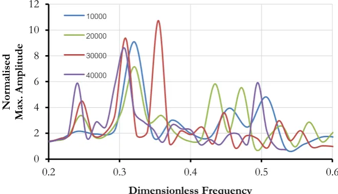
[image:7.595.85.512.604.760.2]Effect of soil modulus on non-dimensional frequency-amplitude response curve is presented in Figs. 4 and 5 for series and parallel arrangement respectively. It is observed that for parallel arrangement, the peaks are observed at nearly constant non-dimensional frequency with variation in soil modulus. The average non-dimensional frequencies corresponding to first three peaks are 0.243, 0.314 and 0.365. But in case of series arrangement, the frequency ratios are observed to be decreasing with soil modulus.
Fig. 4. Effect of Soil modulus on Frequency-Amplitude response Curve for two pile in series arrangement and s/D=3.
Fig. 5. Effect of Soil modulus on Frequency-Amplitude response Curve for two pile in parallel arrangement and s/D=3.
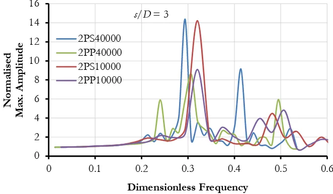
Effect of pile arrangement on non-dimensional frequency-amplitude response curve is presented in Figs. 6 and 7. Comparisons at two different pile spacing 3D and 7D (Es=30000 kPa) are presented in Fig. 6. It is observed that frequencies in the parallel arrangement are higher than those compared to series arrangement. This suggests higher soil stiffness offered in case of parallel configuration. Similar comparison at two different soil modulus (Es=10000 kPa and Es=40000 kPa) for s/D=3 is presented in Fig. 7 which also shows similar trend with respect to arrangement of piles.
0 2 4 6 8 10 12 14 16
0.2 0.3 0.4 0.5 0.6
N
orm
al
ise
d
M
ax
. Am
pl
it
ud
e
Dimensionless Frequency 10000
20000 30000 40000
0 2 4 6 8 10 12
0.2 0.3 0.4 0.5 0.6
N
orm
al
ise
d
M
ax
. Am
pl
it
ud
e
Dimensionless Frequency 10000
[image:8.595.133.463.410.600.2]Fig. 6. Effect of pile arrangement on Frequency-Amplitude response Curve for Es=30000 kPa.
Fig. 7. Effect of pile arrangement on Frequency-Amplitude response Curve for s/D=3.
6.
Conclusions
1) Fundamental frequency is decreasing with increase in pile spacing for piles in series arrangement whereas marginal reduction is observed for piles in parallel arrangement.
2) Maximum amplitude is a complex phenomenon and depends on stiffness of pile soil system, the external frequency and natural frequency. Mass involved in vibration is major governing factor.
3) The fundamental frequency increases with increase in the soil modulus.
4) It is observed that frequencies in the parallel arrangement are higher than those compared to series arrangement.
0 2 4 6 8 10 12
0.1 0.2 0.3 0.4 0.5 0.6
N
orm
al
ise
d
M
ax
. Am
pl
it
ud
e
Dimensionless Frequency
Es=30000 kPa
2PS3D 2PP3D 2PS7D 2PP7D
0 2 4 6 8 10 12 14 16
0 0.1 0.2 0.3 0.4 0.5 0.6
N
orm
al
ise
d
M
ax
. Am
pl
it
ud
e
Dimensionless Frequency
s/D = 3 2PS40000
[image:9.595.132.463.336.529.2]References
[1] H. G. Poulos, “Behavior of laterally loaded piles-I: Single piles,” J. Soil Mech. and Found. Div., vol. 97, no. 5, pp. 711–731, 1971.
[2] P. J. Pise, “Laterally loaded piles in a two-layer soil system,” J. Geotech. Engrg. Div., vol. 108, no. 9, pp. 1177–1181, 1982.
[3] M. F. Randolph, “The response of flexible piles to lateral loading,” Geotechnique, vol. 31, no. 2, pp. 247–259, 1981.
[4] L. C. Reese and H. Matlock, “Non-dimensional solutions for laterally loaded piles with soil modulus assumed proportional to depth,” in Proc. of 8th Texas Conf. on Soil Mechanics and Foundation Engineering, Austin, Texas, 1956, pp. 1–23.
[5] H. Matlock and L. C. Reese, “Generalized solutions for laterally loaded piles,” Journal of Soil Mechanics and Foundation, vol. 86, no. 5, pp. 63–91, 1960.
[6] M. T. Davisson and H. L. Gill, “Laterally loaded piles in a layered soil system,” J. Soil Mech. and Found. Div., vol. 89, no. 3, pp. 63–94, 1963.
[7] H. Matlock, “Correlations for design of laterally loaded piles in soft clay,” in Proc. of 2nd Offshore Technology Conf., Houston, 1970, pp. 577–594.
[8] L. C. Reese and R. C. Welch, “Lateral loading of deep foundations in stiff clay,” J. Geotech. Engrg. Div., vol. 101, no. 7, pp. 633–649, 1975.
[9] M. Novak, “Dynamic stiffness and damping of piles,” Canadian Geotechnical J., vol. 11, pp. 4, pp. 574-598, 1974.
[10] O. I. Ghazzaly, S. T. Hwonc, and M. W. O’Neil, “Approximate analysis of a pile under dynamic, lateral loading,” Computers and Structures, vol. 6, pp. 363-368, 1976.
[11] M. M. Ettouney, J. A. Brennan, and M. F. Forte, “Dynamic behavior of pile groups,” Journal of Geotechnical Engineering, vol. 109, no. 3, pp. 301-317, 1983.
[12] G. Gazetas, “Seismic response of end-bearing single piles,” Soil Dynamics and Earthquake Engineering, vol. 3, no. 2, pp. 82-93, 1984.
[13] T. Nogami and K. Konagai, “Time domain flexural response of dynamically loaded single piles,”
Journal of Engineering Mechanics, vol. 114, no. 9, pp. 1512-1225, 1988.
[14] T. Nogami, J. Otani, K. Konagai, and H. L. Chen, “Nonlinear soil-pile interaction model for dynamic lateral motion,” Journal of Geotechnical Engineering, vol. 118, no. 1, pp. 89-106, 1992.
[15] G. Gazetas, K. Fan, and A. Kaynia, “Dynamic response of pile groups with different configurations,”
Soil Dynamics and Earthquake Engineering, vol. 12, pp. 239-257, 1993.
[16] M. H. El Naggar and M. Novak, “Nonlinear lateral interaction in pile dynamics,” Soil Dynamics and Earthquake Engineering, vol. 14, pp. 141-157, 1995.
[17] D. Badoni and N. Makris, “Nonlinear response of single piles under lateral inertial and seismic loads,”
Soil Dynamics and Earthquake Engineering, vol. 15, pp. 29-43, 1996.
[18] T. Nogami and M. Novak, “Soil-pile interaction in vertical vibration,” Int. J. of Earthquake Eng. and Structural Dynamics, vol. 4, pp. 77-293, 1976.
[19] M. Novak and T. Nogami, “Soil-pile-interaction in horizontal vibration," Earthquake Eng. and Structural Dynamics,” vol. 5, pp. 263-281, 1977.
[20] T. Chau and X. Yang, “Nonlinear interaction of soil–pile in horizontal vibration,” Journal of Engineering Mechanics, vol. 131, no. 8, pp. 847-858, 2005.
[21] Y. X. Cai, P. L. Gould, and C. S. Desai, “Nonlinear analysis of 3D seismic interaction of soil–pile– structure systems and application,” Engineering Structures, vol. 22, pp. 191–199, 2000.
[22] B. K. Maheshwari and P. K. Emani, “Effect of nonlinearity on the dynamic behavior of pile groups,” in the 14th World Conference on Earthquake Engineering, Beijing, China, Oct. 12-17, 2008.
[23] P. K. Emani and B. K. Maheshwari, “Dynamic impedances of pile groups with embedded caps in homogeneous elastic soils using CIFECM,” Soil Dynamics and Earthquake Engineering, vol. 29, pp. 963– 973, 2009.