Determination of Compressive Strength of Concrete by Statistical Learning Algorithms

Article

Determination of Compressive Strength of Concrete

by Statistical Learning Algorithms

Pijush Samui

Centre for Disaster Mitigation and Management, VIT University,Vellore, India E-mail: [email protected]

Abstract. This article adopts three statistical learning algorithms: support vector machine (SVM), lease square support vector machine (LSSVM), and relevance vector machine (RVM), for predicting compressive strength (fc) of concrete. Fly ash replacement ratio (FA),

silica fume replacement ratio (SF), total cementitious material (TCM), fine aggregate (ssa), coarse aggregate (ca), water content (W), high rate water reducing agent (HRWRA), and age of samples (AS) are used as input parameters of SVM, LSSVM and RVM. The output of SVM, LSSVM and RVM is fc. This article gives equations for prediction of fc of concrete.

A comparative study has been carried out between the developed SVM, LSSVM, RVM and Artificial Neural Network (ANN). This article shows that the developed SVM, LSSVM and RVM models are practical tools for the prediction of fc of concrete.

Keywords: Support vector machine, least square support vector machine, relevance vector machine, compressive strength, concrete.

ENGINEERING JOURNAL Volume 17 Issue 1 Received 18 July 2012

1.

Introduction

In the last years, a number of efficient statistical learning algorithms, e.g. support vector machine (SVM) [1, 2], least square support vector machine (LSSVM) [3], and relevance vector machine (RVM) [4] have been proposed. Successful applications of statistical learning algorithms have been reported for various fields [5-7]. This article adopts SVM, LSSVM and RVM for determination compressive strength (fc) of concrete.

SVM was developed by Vapnik and his coworkers in 1995, and it is based on the structural risk minimization (SRM) principle. LSSVM is proposed by taking with equality instead of inequality constraints to obtain a linear set of equations instead of a quadratic programming (QP) problem in the dual space [3, 8]. RVM is a sparse method for training generalized linear models [4]. It can be seen as probabilistic version of SVM. This study uses the database collected by Pala et al. [9]. Table 1 shows the dataset. The database contains information about fly ash replacement ratio (FA), silica fume replacement ratio (SF), total cementitious material (TCM), fine aggregate (ssa), coarse aggregate (ca), water content (W), high rate water reducing agent (HRWRA), age of samples (AS) and fc. A comparative study has been carried out between

[image:2.595.88.506.320.766.2]

the developed SVM, LSSVM and RVM models. The developed SVM, LSSVM and RVM provide equations for the prediction of fc.

Table 1. Dataset used in this study.

FA

(%) (%) SF (kg/mTCM 3_{) (kg/m}ssa 3_{) (kg/m}ca 3_{) (lt/m}W 3₎ HRWRA _(lt/m3_{) (days)} Age _(MPa) fc

0 0 500 724 1086 150 7.5 3 64.9

0 0 500 724 1086 150 7.5 7 75.5

0 0 500 724 1086 150 7.5 28 86.8

0 0 500 724 1086 150 7.5 56 87.2

0 0 500 724 1086 150 7.5 90 95.7

0 0 500 724 1086 150 7.5 180 97.7

15 0 500 700 1086 150 7.5 3 52.1

15 0 500 700 1086 150 7.5 7 66.4

15 0 500 700 1086 150 7.5 28 86

15 0 500 700 1086 150 7.5 56 94.8

15 0 500 700 1086 150 7.5 90 99.6

15 0 500 700 1086 150 7.5 180 106.3

25 0 500 683 1086 150 9.25 3 48

25 0 500 683 1086 150 9.25 7 65.7

25 0 500 683 1086 150 9.25 28 85.4

25 0 500 683 1086 150 9.25 56 90.4

25 0 500 683 1086 150 9.25 90 95.4

25 0 500 683 1086 150 9.25 180 107.8

45 0 500 650 1086 150 10.5 3 34.1

45 0 500 650 1086 150 10.5 7 49.2

45 0 500 650 1086 150 10.5 28 71.8

45 0 500 650 1086 150 10.5 56 85.4

45 0 500 650 1086 150 10.5 90 87.7

45 0 500 650 1086 150 10.5 180 97.7

55 0 500 634 1086 150 13 3 22.3

55 0 500 634 1086 150 13 28 57.4

55 0 500 634 1086 150 13 56 66.6

55 0 500 634 1086 150 13 90 72.8

55 0 500 634 1086 150 13 180 79.9

0 5 500 719 1086 150 8 3 58.3

0 5 500 719 1086 150 8 7 75.5

0 5 500 719 1086 150 8 28 87.8

0 5 500 719 1086 150 8 56 93.1

0 5 500 719 1086 150 8 90 93.6

0 5 500 719 1086 150 8 180 99.3

20 5 500 686 1086 150 9.25 3 46.3

20 5 500 686 1086 150 9.25 7 65.6

20 5 500 686 1086 150 9.25 180 95.9

40 5 500 654 1086 150 11 3 30.5

40 5 500 654 1086 150 11 7 48.6

40 5 500 654 1086 150 11 56 80

40 5 500 654 1086 150 11 90 83.4

40 5 500 654 1086 150 11 180 88.3

0 0 400 710 1157 160 4 3 35

0 0 400 710 1157 160 4 28 60.7

0 0 400 710 1157 160 4 56 67.1

0 0 400 710 1157 160 4 90 70.5

0 0 400 710 1157 160 4 180 70.6

15 0 400 690 1157 160 4.4 3 29.3

15 0 400 690 1157 160 4.4 28 56

15 0 400 690 1157 160 4.4 56 63.4

15 0 400 690 1157 160 4.4 90 68.5

15 0 400 690 1157 160 4.4 180 72.1

25 0 400 660 1157 160 4.8 3 24.7

25 0 400 660 1157 160 4.8 7 33.7

25 0 400 660 1157 160 4.8 28 49.3

25 0 400 660 1157 160 4.8 56 60.8

25 0 400 660 1157 160 4.8 90 66.2

25 0 400 660 1157 160 4.8 180 70.2

45 0 400 634 1157 160 5.2 3 14.5

45 0 400 634 1157 160 5.2 7 20.3

45 0 400 634 1157 160 5.2 28 43.9

45 0 400 634 1157 160 5.2 90 61.2

45 0 400 634 1157 160 5.2 180 63.7

55 0 400 621 1157 160 5.5 3 13.6

55 0 400 621 1157 160 5.5 7 19.8

55 0 400 621 1157 160 5.5 28 37.3

55 0 400 621 1157 160 5.5 56 47.1

55 0 400 621 1157 160 5.5 180 63.2

0 5 400 688 1157 160 5.5 3 37.3

0 5 400 688 1157 160 5.5 7 53

0 5 400 688 1157 160 5.5 28 69.4

0 5 400 688 1157 160 5.5 56 72.1

0 5 400 688 1157 160 5.5 180 74.5

20 5 400 662 1157 160 5.5 3 28.9

20 5 400 662 1157 160 5.5 7 42.1

20 5 400 662 1157 160 5.5 28 62.3

20 5 400 662 1157 160 5.5 56 69.9

20 5 400 662 1157 160 5.5 90 72.4

40 5 400 636 1157 160 6 3 14.5

40 5 400 636 1157 160 6 7 20.5

40 5 400 636 1157 160 6 28 44.6

40 5 400 636 1157 160 6 56 55.3

40 5 400 636 1157 160 6 90 59.1

40 5 400 636 1157 160 6 180 68.4

0 0 410 609 1132 205 0 3 26.1

0 0 410 609 1132 205 0 7 36.9

0 0 410 609 1132 205 0 28 50.8

0 0 410 609 1132 205 0 56 57.1

0 0 410 609 1132 205 0 90 58.1

0 0 410 609 1132 205 0 180 60.6

15 0 410 589 1132 205 0 3 23.3

15 0 410 589 1132 205 0 7 32.3

15 0 410 589 1132 205 0 28 48.9

15 0 410 589 1132 205 0 56 55.7

15 0 410 589 1132 205 0 90 62.6

25 0 410 576 1132 205 0 3 18.4

25 0 410 576 1132 205 0 7 26.2

25 0 410 576 1132 205 0 28 41.7

25 0 410 576 1132 205 0 56 49.1

25 0 410 576 1132 205 0 90 53.7

25 0 410 576 1132 205 0 180 57.9

45 0 410 549 1132 205 0 3 13.4

45 0 410 549 1132 205 0 28 35.6

45 0 410 549 1132 205 0 56 47

45 0 410 549 1132 205 0 90 54.1

45 0 410 549 1132 205 0 180 56.6

55 0 410 536 1132 205 0 3 7.8

55 0 410 536 1132 205 0 7 11.3

55 0 410 536 1132 205 0 28 24

55 0 410 536 1132 205 0 56 33.7

55 0 410 536 1132 205 0 180 48.4

0 5 410 605 1132 205 0 3 27.4

0 5 410 605 1132 205 0 7 39.2

0 5 410 605 1132 205 0 28 57.3

0 5 410 605 1132 205 0 56 59.6

0 5 410 605 1132 205 0 90 67.3

0 5 410 605 1132 205 0 180 66.3

20 5 410 578 1132 205 0 3 20.1

20 5 410 578 1132 205 0 28 52.9

20 5 410 578 1132 205 0 56 60.7

20 5 410 578 1132 205 0 180 68

40 5 410 552 1132 205 0 3 11.4

40 5 410 552 1132 205 0 7 11.68

40 5 410 552 1132 205 0 28 38.7

40 5 410 552 1132 205 0 90 48.7

40 5 410 552 1132 205 0 180 58.4

20 5 410 578 1132 205 0 90 63.7

40 5 500 654 1086 150 11 28 71.1

45 0 400 634 1157 160 5.2 56 54.1

0 0 400 710 1157 160 4 7 48.4

15 0 400 690 1157 160 4.4 7 39.9

45 0 410 549 1132 205 0 7 18.4

55 0 500 634 1086 150 13 7 36.4

20 5 410 578 1132 205 0 7 30.6

55 0 400 621 1157 160 5.5 90 52.9

0 5 400 688 1157 160 5.5 90 73.7

40 5 410 552 1132 205 0 56 45.9

55 0 410 536 1132 205 0 90 41.4

20 5 400 662 1157 160 5.5 180 76

20 5 500 686 1086 150 9.25 56 85.8

2.

Details of SVM

SVM uses the following expression for the prediction of output variable (y):

 

x

b

w

y



.





₍₁₎

where



 

x

expresses the high-dimensional feature space which is nonlinearly mapped from the input space x, b is bias and w is weight.

This article adopts FA, SF, TCM, ssa, ca, W, HRWRA, and AS as input variables. The output of SVM is fc. Thus



FA

SF

TCM

ssa

ca

HRWRA

AS



 

f

c

y



.

The value of w and b have been estimated by minimizing the regularized risk function,

Minimize:





 







N

i

i i

f

x

y

L

N

C

w

1 2

1

2

1



 





_{ }

 

















others





 i i i i i i

x

f

y

x

f

y

x

f

y

L

,

0

(2)

where

L

_



y

_i

,

f

 

x

_i



is ε-insensitive loss function and ε is error insensitive zone. To minimize the effect of noise data, positive slack variables (



_i and *

i



) have added in Eq. (2).

Minimize:













N i i i

N

C

w

1 * 2

1

2

1

_

_

Subjected to:

y

i



w

.



 

x

i



b









i

 

*

. x_i b y_{i i} w



  







0



i





_i*0 (3)

By introducing kernel function

K



x

i

,

x

j



, the above optimization problem (3) can be written in the following way [1]:

Maximize:

























          N i N j N i N i i i i i i j i j j i

i K x x y

1 1 1 1

* * * * , . 2

1

_

_

_

_

_

_

_

_

_

Subject to:













N i i i 1 *

0





(4)



_i,



_i*

 

0,C

where



i,

* i



are Lagrange multipliers. The final equation of SVM takes the following form:



















N i i i

i

K

x

x

b

y

1

*

,





(5)

To develop the SVM, the data have been divided into the following groups:

 Training dataset: This is required to construct the SVM model. This article uses the same training dataset as used by Pala et al. [9].

 Testing Dataset: This is required to verify the developed SMV. This article uses the same testing dataset as used by Pala et al. [9].

This study adopts the radial basis function:





























_

_





₂

2

exp

,



x

x

x

x

x

x

K

k T k

where σ is the width of radial basis function and T is transpose) as kernel function. The data have been normalized between 0 and 1. The program of SVM has been constructed by using MATLAB.

3.

Details of RVM

RVM uses the following equation for the prediction of output (y).

 

_















n i i i

K

x

x

a

a

x

a

y

1 0

,



(6)

where x is input, K(x, xi) is kernel function, n is number of data and a is weight. In this study,



FA

SF

TCM

ssa

ca

HRWRA

AS



x



,

,

,

,

,

,

and

 

f

c

y



The likelihood of the complete data set can be written as



  













_

_



 2

2 2 2 2

2

1

exp

2

y

aφ

σ

πσ

y|a,σ

p

n (7)

To prevent overfitting, automatic relevance detection (ARD) prior is set over the weights.

 

_





_

 

               n i n i j i i i i a p 0 0 2 1 2 exp 2 ,

0















(8)

where α is a hyperparameter vector that controls how far from zero each weight is allowed to deviate [10]. The posterior distribution over the weights is thus given by:



 

_



 

_

 

 

_

_{ }

_

   _{ } _{ }   

_

  

_



_













a a

y p a p a y p y a

p n 1 2 12 1

2 2 2 2 1 exp 2 , , ,

, (9)

where the posterior covariance and mean are respectively:



_2



1













A

(10)

y









2



For uniform hyperpriors over α and σ2, one needs only maximize the term

p



y

α

,σ

2



:



 



 

 









_

















_







    



y

A

I

y

A

I

a

p

a

y

p

y

p

n _{2 1} 1_{2 2 1} 1

2 2 2

2

1

exp

2

,

,















(11)

vectors.

This study adopts the same training dataset, testing dataset, kernel function and normalization technique for the RVM as used by the SVM. MATLAB has been used to develop RVM.

4.

Details of LSSVM

LSSVM adopts the following equation for prediction of output (y)

 

x

b

w

y



T





₍₁₂₎

where w is weight, b is bias, x is input variable and φ(x) is non-linear mapping function. In this study,



FA

SF

TCM

ssa

ca

HRWRA

AS



x



,

,

,

,

,

,

and

 

f

c

y



_.

LSSVM uses the following optimization problem determination of w and b:

Minimize:







N

k k T

e

w

w

1 2

2

1

2

1

_

Subject to:

 

 

k k T

e b x w x

y 



  , k = 1, …, N. (13) where ek is the random errors and γ is a regularization parameter in determining the trade-off between

minimizing the training errors and minimizing the model complexity.

The following equation has been obtained by solving the above optimization problem and it has been used for prediction of fc [15, 16]:















N

k

k k

c

y

K

x

x

b

f

1

,



(14)

where

K



x

,

x

k



is kernel function and αk is lagrange multipliers.

This study adopts the same training dataset, testing dataset, kernel function and normalization technique for the LSSVM as used by the SVM and RVM. The program of LSSVM has been constructed by MATLAB.

5.

Results and Discussion

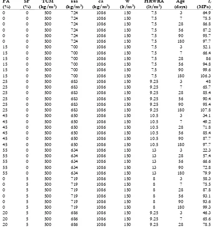
For SVM, the design value of C, ε and σ have been determined by a trial and error approach. The design values of C, ε and σ are 100, 0.01 and 2 respectively. The best SVM produces 115 support vectors. The performance of training and testing dataset has been determined by using the design values of C, ε and σ.

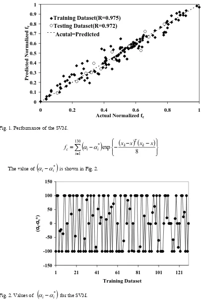
Figure 1 shows the performance of training and testing for the SVM. This article employs coefficient of correlation (R) to assess the performance of SVM. For a good model, the value of R should be close to one. It is observed from Fig. 1 that the value of R is close to one for training as well as testing dataset. So, the developed SVM predicts fc fairly well. The developed SVM presents the following equation (by substituting





























_

_





₂

2

exp

,



x

x

x

x

x

x

K

k

T k

[image:8.595.70.475.75.679.2]

Fig. 1. Performance of the SVM.







 























_

_







130

1

*

8

exp

i

k T k i

i c

x

x

x

x

f





(15)

The value of



*



i i





 is shown in Fig. 2.

Fig. 2. Values of



*



i i





 for the SVM.

[image:8.595.115.479.80.358.2]

In RVM, the trial and error approach has been adopted for determining the design value of σ. The developed RVM gives best performance at σ = 1. Therefore, the design value of σ is 1.

Figure 3 shows performance of RVM model. It is observed from Fig. 3 that the value of R is close to one for training as well as testing dataset. So, the developed RVM has the capability for predicting fc. The

developed RVM gives the following equation for prediction of fc:

0 0.1 0.2 0.3 0.4 0.5 0.6 0.7 0.8 0.9 1

0 0.2 0.4 0.6 0.8 1

Actual Normalized fc

Predi

cted N

orma

li

zed f

c

Training Dataset(R=0.975) Testing Dataset(R=0.972)

Acutal=Predicted

-150 -100 -50 0 50 100 150

1 21 41 61 81 101 121

Training Dataset

(

i

-

i



 























_

_





1

2

exp

i

k k

i c

x

x

x

x

a

f

(16)

6.

Conclusion

This study successfully applied SVM, RVM and LSSVM for the prediction of fc of concrete. 130 datasets

have been utilized to develop the models. User can use the developed equations for practical purposes. The developed RVM, SVM and LSSVM give almost the same performance. The obtained variance from the RVM can be used to determine uncertainty. SVM and RVM produce sparse solutions. In summary, it can be concluded that SVM, RVM and LSSVM can be examined for solving different problems in concrete.

References

[1] V. N. Vapnik, The Nature of Statistical Learning Theory, New York: Springer-Verlag, 1995.

[2] B. Schölkopf, Support Vector Learning, R. Oldenbourg Verlag,M¨unchen. Doktorarbeit, TU Berlin. Online at: http://www.kernel-machines.org.

[3] J. A. K. Suykens, and J. Vandewalle, “Least squares support vector machine classifiers,” Neural Process. Lett., vol. 9, pp. 293-300, 1999.

[4] M. E. Tipping, “The relevance vector machine,” Advances in Neural Information Processing Systems, vol. 12, pp. 652-658, 2000.

[5] D. Zhao, W. Zou, and G. Sun, “A fast image classification algorithm using support vector machine,”

Proceeding 2nd International Conference on Computer Technology and Development, pp. 385-388, 2010.

[6] H. Suetani, A. M. Ideta, and J. Morimoto, “Nonlinear structure of escape-times to falls for a passive dynamic walker on an irregular slope: Anomaly detection using multi-class support vector machine and latent state extraction by canonical correlation analysis,” Proceeding IEEE Int. Conference on Intelligent Robots and Sys., pp. 2715-2722, 2011.

[7] D. Matić, F. Kulić, M. Pineda-Sánchez, and I. Kamenko, “Support vector machine classifier for diagnosis in electrical machines: Application to broken bar,” Expert Syst. Appl., vol. 39, no. 10, pp. 8681-8689, 2012.

[8] J. A. K. Suykens, T. Van Gestel, J. De Brabanter, B. De Moor, and J. Vandewalle, Least Squares Support Vector Machines, Singapore: World Scientific, 2002.

[9] M. Pala, E. Özbay, A. Öztaş, and M. I. Yuce, “Appraisal of long-term effects of fly ash and silica fume on compressive strength of concrete by neural networks,” Constr. Build. Mater., vol. 21, no. 2, pp. 384-394, 2007.

[10] B. Schölkopf, and A. J. Smola, Learning with Kernels: Support Vector Machines, Regularization, Optimization, and Beyond, Cambridge: MIT Press, 2002.

[11] J. O. Berger, Statistical Decision Theory and Bayesian Analysis, 2nd ed., New York: Springer, 1985.

[12] G. A. Wahba, “Comparison of GCV and GML for choosing the smoothing parameters in the generalized spline-smoothing problem,” Ann. Statist., vol. 13, no. 4, pp. 1378-1402, 1985.

[13] D. J. MacKay, “Bayesian methods for adaptive models,” Ph.D. Thesis, California Institute of Technology, 1992. Online at: http://resolver.caltech.edu/CaltechETD:etd-01042007-131447.

[14] M. E. Tipping, “Sparse Bayesian learning and the relevance vector machine,” J. of Machine Learning Research, vol. 1, pp. 211-244, 2001.

[15] V. N. Vapnik, Statistical Learning Theory, New York: Wiley, 1998.