The Fall 2017 issue of the Research Update comes after a very active year at the Banco de España that featured an unusually large number of conferences sponsored, articles and working papers published, and new researchers hired. Our Update aims to inform the academic and policy-making communities about the results of these research efforts.
As usual, this issue of the Research Update includes several feature articles outlining policy-relevant findings from the work of Banco de España researchers. First, an article by M. Correa-López and R. Domenech argues that deregulation of service industries has provided a powerful boost to Spanish manufacturing exports. A second article, by I. Kataryniuk and J. Martínez-Martín, cautions that apparent productivity gains in emerging economies prior to the Great Recession may not prove permanent. A contribution by S. Mayordomo, A. Moreno, S. Ongena, and M. Rodríguez-Moreno analyzes the factors that lead banks to collateralize loans with real assets or personal guarantees, noting that personal guarantees have become much more common since 2011. Next, O. Arce, R. Gimeno, and S. Mayordomo document the effects of the ECB’s recent purchases of bonds of non-financial corporations, showing that these actions not only eased credit conditions for issuers of eligible bonds, but also spilled over via expanded bank lending to other corporations, including small and medium enterprises. Finally, M. Alloza, P. Burriel, and J. Pérez describe a new quarterly fiscal database which they use to measure spillovers of fiscal expansions across several euro area countries.
This Update also documents the conferences that took place at the Banco de España in 2017, including its first Annual Research Conference, its first biennial Conference on Financial Stability, and activities co-organized with the European System of Central Banks (ESCB), the CEPR, the ADEMU network, the Bank of Canada, and the World Bank. We highlight these and other developments at the Banco de España in hopes that they will interest the broader research community, in Spain and internationally, and thereby contribute to an improved understanding of economic policy.
Óscar Arce Ángel Estrada Juan Francisco Jimeno Jesús Saurina
Research Committee, Banco de España
CONTENTS:
Features
/
Publications
/
News and Events
/
People /
Announcements
FEATURES
SERVICE REGULATIONS, INPUT PRICES AND EXPORT VOLUMES: EVIDENCE FROM A PANEL
OF MANUFACTURING FIRMS1
MÓNICA CORREA-LÓPEZ AND RAFAEL DOMÉNECH
WORKING PAPER 1707
Using a panel of firm-level data from Spanish manufacturers, this study shows that better service regulation reduces the price of intermediate inputs paid by downstream firms. The beneficial cost effects of services reforms extend to both large and small-to-medium sized corporations (SMEs), but the former tend to enjoy greater gains. Likewise, in international markets, we identify an input cost channel through which service regulations affect the volume of exports, especially for large manufacturers. Our estimates indicate that, from 1991 to 2007, large firms increased their volume of exports by an average of 22% as a result of the direct input cost effect of services reforms. The firms that benefited the most typically belonged to industries more dependent on services. Furthermore, convergence to the “best practice” regulatory framework in services would have raised exports at least by an additional 10%.
Introduction
Since the 1990s the barriers to competition in certain services activities in the Spanish economy have been progressively lowered. The change in the regulatory framework has involved a substantial reduction in the barriers to entry for new firms, favouring more competitive market structures. As a result, Spanish regulation has moved closer to the best practice framework of the advanced economies (see Chart 1).2
Services have a significant influence on the ability of manufacturing firms to compete both in the domestic market and abroad. This is because services include high-technology activities such as telecommunications, logistics, and engineering services, which play an essential role in improving the efficiency of the industrial sector. Also, competitive strategies in industry, based on product differentiation and quality improvement, largely depend on the availability of specialised business services.
The empirical literature has largely addressed the effects of services deregulation on macroeconomic aggregates, such as growth, employment and inflation.3 More recently, some authors have quantified the economic impact of such reforms on the industrial base of OECD countries.4 Barone and Cingano (2011), for example, find that countries with a more competitive regulatory framework in services have higher growth rates of value added, productivity and exports in those manufacturing industries that make the most intensive use of services. This suggests that services regulation may affect the pattern of specialisation and international trade in the advanced economies. Yet, despite the emerging literature, none of the studies has empirically identified the transmission channel through which downstream firms’ decisions and market outcomes are affected by upstream service regulations, whether this channel operates through, e.g., product innovation, process innovation or input price-setting mechanisms. Using firm-level data from Spanish manufacturers, this article addresses precisely this question and identifies an input cost channel through which service regulations affect manufacturing firms’ export performance.
1 This article is a summary of the research carried out in M. Correa-López and R. Doménech (2017).
2 According to the OECD Product Market Regulation (PMR) indicators. This set of indicators quantifies de jure information on the regulatory environment for different market services in OECD countries. Direct quantification of competition in services (a de facto indicator) is less common in the literature. For further details, see Mora-Sanguinetti and Martínez-Matute (2014).
3 See, for example, Nicoletti and Scarpetta (2003), Griffith
et al. (2007), Fiori et al. (2012) and Correa-López et al. (2014), among others.
4 See, for example, Barone and Cingano (2011) and Bourlès
is built by combining information on the restrictions to competition in the energy, transport, communications and professional services sectors (Zst ), with an estimate ω js of the level of dependence of manufacturing sector j on the output produced of service sector s:6
REGjt=∑s=1..4 ωjs Zst
Chart 2 depicts the evolution of the regulatory impact indicator for each manufacturing sector. The variability shown across sectors and over time reflects differences in the extent of service sector dependence of each industry, in the composition of the input services used, and in the initial level and pace of deregulation of each service.7
Data and econometric strategy
The source of firm-level data is the Encuesta sobre Estatregias Empresariales (ESEE), an annual survey conducted by Fundación SEPI. The total sample comprises 29,137 observations covering information on 3,540 firms arranged in an unbalanced panel observed annually over the period 1991-2007 with an average of 8 observations per firm. Of the total 29,137 observations, 8,980 correspond to large firms (more than 200 employees) and 20,157 to SMEs (10 to 200 employees).
Summary statistics show that, on average, large firms export more, are more efficient and capital intensive, and are less leveraged and older than SMEs.5 They also face a lower inflation rate in intermediates, and have more market power and foreign presence in their ownership structure.
The indicator that measures the impact of the regulatory environment in the upstream market for service inputs on downstream manufacturing (REGjt )
5 See Table 1 of Correa-López and Doménech (2017).
6 The food, non-metallic mineral products and chemicals industries are the most dependent on services (around 15% of total inputs), about three times more than the least dependent industry, electrical and optical equipment.
7 Services reforms were especially pronounced in the energy sector, followed by transport, communication and, to a lesser extent, professional services, while manufacturing dependence on professional services and transport has become increasingly relevant.
SOURCE: OECD.
a The indicator takes values between 0 and 6, with lower values denoting more efficient functioning of the markets.
0 1 2 3 4 5 6 1998 2003 2008 2013
BEST PRACTICES FRAMEWORK SPAIN OECD ADVANCED (MEDIAN)
PROFESSIONAL SERVICES AND RETAIL TRADE
INDICATORS OF REGULATION IN SERVICES (a) CHART 1
0 1 2 3 4 5 6 90 92 94 96 98 00 02 04 06 08 10 12 14
ENERGY: SPAIN AND STATISTICS OF ADVANCED COUNTRIES
0 1 2 3 4 5 6 90 92 94 96 98 00 02 04 06 08 10 12 14
TRANSPORT: SPAIN AND STATISTICS OF ADVANCED COUNTRIES
0 1 2 3 4 5 6 90 92 94 96 98 00 02 04 06 08 10 12 14 WORST PRACTICES FRAMEWORK EUROPEAN ADVANCED (MEDIAN) OECD ADVANCED (MEDIAN) SPAIN
BEST PRACTICES FRAMEWORK
COMMUNICATIONS: SPAIN AND STATISTICS OF ADVANCED COUNTRIES
results of the first step, we instrument the price of intermediate inputs with the regulatory impact indicator. We check for instrument validity and informativeness by adopting an incremental approach whereby the baseline specification is extended with additional determinants and estimated using alternative methods while addressing endogeneity issues.8
We implement a two-step econometric approach to identify the effect of regulation on exports going through the price of intermediate consumption. In the first step, we measure the effect of services regulation on the firm’s price of intermediate inputs, controlling for other firm- and industry-level determinants. This step allows us to evaluate whether service regulation might be considered as a strongly informative instrument for intermediate input prices in the second step, which is a Generalized Method of Moments (GMM) procedure. Throughout the analysis, services reforms are treated as exogenous, derived from EU-wide directives and initiatives. In the second step, we regress the firm’s foreign sales on the price of intermediate consumption. In light of the
8 Our identification strategy consists of evaluating how the use of the regulatory impact indicator as an external instrument influences the coefficient on the price of intermediate consumption. We check for changes in coefficient size and significance both in a baseline model that omits firm attributes and in the full empirical model.
REGULATORY IMPACT INDICATOR (a) CHART 2
0.0 0.1 0.2 0.3 0.4 0.5 0.6 0.7 0.8 90 91 92 93 94 95 96 97 98 99 00 01 02 03 04 05 06 07
FOOD PAPER INDUSTRY CHEMICALS INDUSTRY
OTHER
RUBBER AND PLASTICS
TEXTILES NON-METALLIC MINERAL PRODUCTS BASE METALS ELECTRICAL AND OPTICAL EQUIPMENT
TRANSPORT EQUIPMENT
SOURCE: Authors´ calculations based on OECD data.
a Higher values of the indicator denote a higher impact on manufactures of barriers to competition in the services sector.
SOURCE: Authors´ calculations, based on the ESEE of Fundación SEPI.
a All specifications include a constant, time dummies and industry. *** denotes statistical significance at the 1% level, ** at the 5% level and * at the 10% level, respectively. Figures in brackets are robust standard errors.
Dependent variable: Fixed effects Random effects Fixed effects Random effects Fixed effects Random effects Regressor * * * 4 2 2 . 0 * * * 1 8 1 . 0 * * * 2 6 2 . 0 * * * 8 5 2 . 0 * * * 8 2 2 . 0 * * * 4 8 1 . 0 k r o w e m a rf y r o t a l u g e r n i e g n a h C [0.040] [0.036] [0.073] [0.062] [0.053] [0.045] 0.261*** 0.312*** 0.369*** 0.405*** 0.217*** 0.278*** [0.036] [0.034] [0.063] [0.061] [0.044] [0.042] * * * 7 1 0 . 0 * * 5 1 0 . 0 * * * 2 2 0 . 0 * * 2 2 0 . 0 * * * 8 1 0 . 0 * * * 4 1 0 . 0 s t r o p x e d lr o W [0.006] [0.004] [0.010] [0.006] [0.007] [0.006] 0 0 0 . 0 0 0 0 . 0 * * * 3 0 0 . 0 * * * 2 0 0 . 0 * * 1 0 0 . 0 * * 1 0 0 . 0 s t r o p m i t u p n I [0.001] [0.001] [0.001] [0.001] [0.001] [0.001] 2 0 0 . 0 -* * 3 0 0 . 0 -2 0 0 . 0 -2 0 0 . 0 -* 2 0 0 . 0 -* * 3 0 0 . 0 -n o i s s e c e R [0.001] [0.001] [0.002] [0.002] [0.001] [0.001] Whole sample Large firms SMEs
Change in price of inputs
REGULATION IN SERVICES AND INPUT PRICES Sample of manufacturing firms in Spain, 1991-2007 (a)
TABLE 1
possibly because firms facing weak demand search more intensively for cost-effective suppliers or negotiate lower input prices.
Overall, our results indicate that service sector deregulation reduces the price of intermediate inputs paid by firms and that firm size is relevant for this link. Since the pro-competitive cost effect of deregulation is stronger for large firms than for SMEs, we expect that the impact of service regulations on firms’ exports will be more evident among large firms.
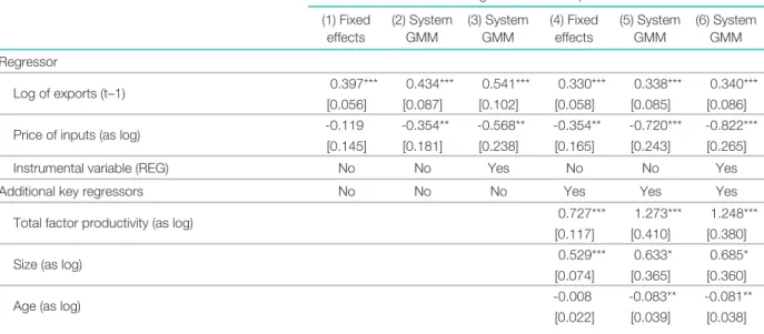
Table 2 shows the second step estimates for the sample of large firms.9 The results confirm that input prices
Results
The results in Table 1 show a positive and significant relationship between the sector-specific change in the regulatory impact indicator and the firm-level rate of variation in the price of intermediate inputs. Considering that Spain undertook major services reforms in the period of study, the estimates indicate that the removal of barriers to competition in services reduced inputs inflation for manufacturers. Quantitatively, the first two columns suggest that increasing the deregulatory effort by 0.1 reduces input price inflation by an average of 2 percentage points. The magnitude of the effect appears to vary with firm size, with an effect of 2.6 percentage points for large firms (columns 3 and 4) and 2 percentage points for SMEs (columns 5 and 6). Small firms could possibly be at a disadvantage with respect to large firms when negotiating the best contract conditions with service providers.
On the other hand, the inflation rate for intermediate inputs of US manufacturing, in world real exports and in import prices are positively and significantly correlated with the inflation rate of intermediate consumption. These results indicate the presence of technology-, supply- and demand-side drivers of intermediate input prices, out of which, the price of intermediates in US manufacturing had the largest influence. Finally, a firm that reports a recession in its main market faces lower intermediates inflation,
9 As an illustrative starting point, we first report the results of the OLS fixed-effects estimator. Then, we employ the System GMM estimator (Arellano and Bover (1995), Blundell and Bond (1998)), which effectively controls for the potential endogeneity of introducing lagged export volumes, input prices and firm-level characteristics in the specification. A common problem with system GMM is instrument proliferation: too many instruments can overfit endogenous variables and fail to remove their endogeneous components. To limit the risk of instrument proliferation, we carefully restrict the number of lags to use as instruments for each endogenous variable and we collapse the instrument matrices, as proposed by Roodman (2009). Note that, unless stated explicitly, the discussed impacts are short-term, given the inclusion of the lagged endogenous variable.
SOURCE: Authors´ calculations, based on the ESEE of Fundación SEPI.
a All specifications include a constant, time dummies and industry. *** denotes statistical significance at the 1% level, ** at the 5% level and * at the 10% level, respectively. Figures in brackets are robust standard errors. See Correa-López and Doménech (2017) for a complete list of regressors.
(1) Fixed effects (2) System GMM (3) System GMM (4) Fixed effects (5) System GMM (6) System GMM Regressor 0.397*** 0.434*** 0.541*** 0.330*** 0.338*** 0.340*** [0.056] [0.087] [0.102] [0.058] [0.085] [0.086] -0.119 -0.354** -0.568** -0.354** -0.720*** -0.822*** [0.145] [0.181] [0.238] [0.165] [0.243] [0.265] s e Y o N o N s e Y o N o N ) G E R ( e l b a ir a v l a t n e m u r t s n I s e Y s e Y s e Y o N o N o N s r o s s e r g e r y e k l a n o it i d d A 0.727*** 1.273*** 1.248*** [0.117] [0.410] [0.380] 0.529*** 0.633* 0.685* [0.074] [0.365] [0.360] -0.008 -0.083** -0.081** [0.022] [0.039] [0.038] Logarithm of real exports
Dependent variable:
Price of inputs (as log)
Total factor productivity (as log) Size (as log)
Log of exports (t–1)
Age (as log)
REGULATION IN SERVICES AND SALES ABROAD, LARGE FIRMS
have a significant negative effect on the export volumes of large manufacturing firms. The inclusion of the regulatory impact indicator in the provision of services as an explanatory factor increases this effect (columns 3 and 6).10 Thus, the study identifies the presence of a transmission channel of services reforms to exports that works through the input costs borne by firms. With regard to other determinants, in addition to the importance of the persistence mechanisms, the results indicate that firm size and productivity, in particular, have a significant positive effect on exports. Hence, according to the baseline results shown in column 6, a 1% rise in productivity is associated with an increase of 1.2% in exports, and a 1% increase in firm size raises exports by 0.7%. In contrast, there is a negative correlation between firm’s age and export activity, which could indicate that the expansion strategy of younger firms is focused on growth in foreign markets. Capital intensity, market share, long-term debt, and foreign ownership are not found to be significant determinants of the volume of exports.
In the case of SMEs, the results shown in Table 3 confirm the significant negative effect of input prices on exports. However, the importance of the transmission channel of services reforms that operates through input costs is less evident from an empirical standpoint and is confined to the model in column 3. Table 3 reveals the relevance of size and, especially, TFP for the export performance of SMEs, with point elasticities of 0.9 and 2.4 per cent, respectively. Likewise, the results show that the SMEs reporting a recessionary main market witnessed a significant rise of their sales abroad. In addition, the estimates suggest that the age of the firm and the number of industrial establishments are negatively associated to the volume of exports.
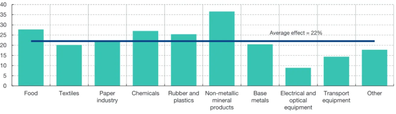
Finally, we carry out two simulation exercises that tentatively illustrate the impact on firm-level manufacturing exports of adopting a more efficient regulatory framework in upstream services (see Chart 3). To this end, we take the empirical model of large firms shown in column 6 of Table 2 as the baseline and, in line with that model, the long-term elasticity of exports to the price of intermediate inputs is set at 1.25%.
SOURCE: Authors´ calculations based on the ESEE of Fundación SEPI.
0 5 10 15 20 25 30 35 40
Food Textiles Paper
industry Chemicals Rubber andplastics Non-metallicmineral products
Base
metals Electrical andoptical equipment
Transport
equipment Other
EFFECT OF CONVERGENCE TOWARDS THE BEST PRACTICES FRAMEWORK, 1991-2007 Total change as percent by industry
Average effect = 9.8%
SIMULATION EXERCISE ON TOTAL EXPORTS OF LARGE FIRMS CHART 3
0 5 10 15 20 25 30 35 40
Food Textiles Paper
industry Chemicals Rubber andplastics Non-metallicmineral products
Base
metals Electrical andoptical equipment
Transport
equipment Other
EFFECT OF REFORMS IN THE REGULATORY FRAMEWORK OF THE SERVICES SECTOR COMPARED WITH A SCENARIO OF NO REFORMS, 1991-2007 Total change as percent by industry
Average effect = 22%
10 It also improves the model’s significance and exogeneity tests. For further details, see Correa-López and Doménech (2017).
The simulation exercise suggests that the improved regulatory practices in services activities had a strong impact on the input prices faced by firms, which would have increased by 17.7% more had there been no such improvement between 1991 and 2007. According to these estimates, the effect of services reforms channelled through the price of intermediate consumption increased exports by 22%, on average, compared with a hypothetical scenario of no reforms. Consistent with Chart 2, the firms that benefited the most belonged to industries typically more dependent on service inputs. On the other hand, had regulation moved closer to the best practice framework in 2007, the export volume of large firms would have been 9.8% higher, on average, than it actually was.11
Conclusion
Growing evidence suggests that regulatory barriers to competition in inputs markets matter for the performance of downstream firms. In this article, we
estimate the impact of barriers to competition in services on the cost of inputs and the export performance of manufacturing firms in Spain, finding a significant impact on exports, especially for larger firms. Our estimates suggest that additional gains in the degree of competition could further improve the export performance of the Spanish economy.
REFERENCES
ARELLANO, M., and O. BOVER (1995). “Another look at the instrumental variable estimation of error-components models”, Journal of Econometrics, vol. 68, pp. 29-51.
BARONE, G., and F. CINGANO (2011). “Service regulation and growth: evidence from OECD countries”, Economic Journal, vol. 121, pp. 931-957.
BLUNDELL, R., and S. BOND (1998). “Initial conditions and moment restrictions in dynamic panel data models”, Journal of Econometrics, vol. 87, pp. 115-143.
BOURLÈS, R., G. CETTE, J. LOPEZ, J. MAIRESSE and G. NICOLETTI (2013). “Do product market regulations in upstream sectors curb productivity growth? Panel data evidence for OECD Countries”. Review of Economics and Statistics, vol. 95, pp. 1750-1768.
11 The best practices framework reflects average regulation in the three OECD countries whose regulatory framework is most conducive to competition.
SOURCE: Authors´ calculations, based on the ESEE of Fundación SEPI.
a All specifications include a constant, time dummies and industry. *** denotes statistical significance at the 1% level, ** at the 5% level and * at the 10% level, respectively. Figures in brackets are robust standard errors. See Correa-López and Doménech (2017) for a complete list of regressors.
(1) Fixed effects (2) System GMM (3) System GMM (4) Fixed effects (5) System GMM (6) System GMM Regressor 0.482*** 0.465*** 0.480*** 0.407*** 0.352*** 0.371*** [0.027] [0.047] [0.047] [0.028] [0.064] [0.062] -0.152 -0.410* -0.578** -0.712*** -0.863* -0.859* [0.179] [0.235] [0.228] [0.159] [0.442] [0.450] s e Y o N o N s e Y o N o N ) G E R ( e l b a ir a v l a t n e m u r t s n I s e Y s e Y s e Y o N o N o N s r o s s e r g e r y e k l a n o it i d d A 0.811*** 2.081*** 2.380*** [0.099] [0.708] [0.689] 0.667*** 0.989*** 0.892*** [0.080] [0.226] [0.204] -0.019 -0.120** -0.114** [0.037] [0.056] [0.054] -0.087*** 0.784 1.076** [0.034] [0.532] [0.459] -0.173 -0.383*** -0.347*** [0.106] [0.109] [0.101] Number of establishments
Total factor productivity (as log) Size (as log)
Age (as log)
Logarithm of real exports
Log of exports (t–1) Price of inputs (as log)
Recession
Dependent variable:
REGULATION IN SERVICES AND SALES ABROAD, SMEs
product and labour market reforms: are there synergies?”, Economic Journal, vol. 122, pp. F79–F104.
GRIFFITH, R., R. HARRISON and G. MACARTNEY (2007). “Product market reforms, labour market institutions and unemployment”, Economic Journal, vol. 117, pp. 142-66.
MORA-SANGUINETTI, J. S., and M. MARTÍNEZ-MATUTE (2014). “La regulación en el mercado de productos en España según los indicadores de la OCDE”. Boletín Económico, December, Banco de España.
ROODMAN, D. (2009). “Practitioners’ corner: A note on the theme of too many instruments”, Oxford Bulletin of Economics and Statistics, vol. 71, pp. 135-158.
CONWAY, P., and G. NICOLETTI (2006). “Product market regulation in the non-manufacturing sectors of OECD countries: measurement and highlights”, Working Paper 58, Economics Department OECD. CORREA-LÓPEZ, M., and R. DOMÉNECH (2017).
“Service regulations, input prices and export volumes: Evidence from a panel of manufacturing firms”, Banco de España Working Paper 1707. CORREA-LÓPEZ, M., A. GARCÍA-SERRADOR and
C. MINGORANCE-ARNÁIZ (2014). “Product Market Competition, Monetary Policy Regimes and Inflation Dynamics: Evidence from a Panel of OECD Countries”, Oxford Bulletin of Economics and Statistics, vol. 76, pp. 484-509.
FIORI, G., G. NICOLETTI, S. SCARPETTA and F. SCHIANTARELLI (2012). “Employment effects of
TFP GROWTH AND COMMODITY PRICES IN EMERGING ECONOMIES
IVÁN KATARYNIUK AND JAIME MARTÍNEZ-MARTÍN
WORKING PAPER 1711
Total Factor Productivity (TFP) growth in emerging economies has been falling in the last few years, particularly in commodity-exporting economies. In this paper, we explore different determinants of TFP growth in the short run and find that shocks in commodity prices have been highly correlated with the evolution of productivity, although the recent decline has been also related to negative supply shocks.
Total Factor Productivity (TFP) is an important but poorly understood driving force of economic growth, defined as a residual after growth by means of factor accumulation, both in labor and in capital, is eliminated. Therefore it is especially relevant when factor accumulation is subdued (Easterly and Levine, 2001). In this regard, many commodity-exporting emerging economies (EMEs) are undergoing a process of adjustment of their potential output. This coincides with a decline in commodity prices, after a period in which commodity prices and economic activity both grew rapidly. This phenomenon has been documented by several related papers, either for EMEs in general (Tsounta, 2014) or for economic or geographical areas (Sosa et al., 2013, for Latin America, or Anand et al., 2014, for East Asia).
In the long run, one might expect that commodity prices should not have any effect on potential output. However, their effect in the short and medium run is less clear. Shifts in commodity prices may either alter investment decisions or generate labor force reallocations toward different sectors. Moreover, complementarities between commodity sectors and manufacturing/services sectors could lead to a positive correlation of TFP and commodity prices in the short run (Ferraro and Peretto, 2015). In this regard, recent studies show that some sectors, especially non-tradables, have been positively affected by commodity price booms (De la Huerta and García-Cicco, 2016). To better understand TFP, the recent evolution of commodity exporters is an interesting case to study, as their TFP growth plummeted at the same time that international prices of most commodities suffered huge corrections (see Figure 1).
Methodology and selection of variables
This study aims to analyze empirically the cross-country impact of commodity prices shocks on aggregate TFP growth for a sample of EMEs. First, under a growth accounting framework with a Cobb-Douglas production
COMMODITY PRICES INFLATION AND TFP GROWTH (%) FIGURE 1
-10 -5 0 5 10
1 ARGENTINA 2 BOLIVIA 3 BRAZIL
-40 -20 0 20 40 4 CHILE -10 -5 0 5 10
5 COLOMBIA 6 ECUADOR 7 INDONESIA
-40 -20 0 20 40 8 PERU -10 -5 0 5 10
9 RUSSIA 10 SAUDI ARABIA 11 SOUTH AFRICA
-40 -20 0 20 40 12 URUGUAY 00 02 04 06 08 10 12 14 00 02 04 06 08 10 12 14 00 02 04 06 08 10 12 14 00 02 04 06 08 10 12 14
function (calculating TFP as the growth residual after taking into account labor units and physical capital), we estimate country-specific annual TFP growth (1992-2014).
Second, we construct country-specific commodity prices indices and we use a Bayesian Model Averaging (BMA) approach1 to select a static model that explains TFP growth on the basis of a pool of variables used in the literature, including cyclical variables, such as output and credit gaps (constructed as the cyclical components of output and credit after HP filtering), as well as structural variables, in order to test whether commodity prices growth is robustly correlated with TFP growth. The results of the BMA estimation suggest that fluctuations of commodity export prices in commodity-exporting countries are a robust predictor of TFP variation.2 Also, TFP is found to be strongly cyclical, as demonstrated by the substantial explanatory power of the output gap for TFP. The empirical results imply that a decrease of 10% in commodity prices is associated with a drop of around 0.6-1.0 percentage points of TFP growth per year for an average commodity-exporting EME. Other variables selected under a random-effects estimation are discarded once the existence of fixed effects is taken into account.
Using the findings of the previous part, in a third step we address endogeneity, and the dynamic behavior of the variables, in order to identify the effects of structural shocks. We propose a panel Bayesian VAR, based on Canova and Ciccarelli (2013), and we introduce cross-sectional heterogeneity as in Jarocinski (2010). For each country unit i we estimate:
where y i,t is a vector of endogenous regressors including the output gap and TFP growth, and x i, t is a vector of exogenous variables including commodity prices growth.
Our structural analysis is restricted to nine commodity-exporting EMEs (Brazil, Bolivia, Chile, Colombia, Ecuador, Indonesia, Peru, South Africa, and Uruguay) over the period 1992-2014. This sample is chosen due to computational restrictions, and to ensure comparability, as our modelling approach generates a common steady state for all country units.3
In order to identify shocks in the endogenous variables, we rely on a Cholesky ordering of the output gap and TFP growth. In principle, the output gap should capture business cycle fluctuations more related with demand shocks, which usually fade away in the medium run. By contrast, TFP growth ought to capture supply shocks, with a permanent effect, even though we have seen that other factors help explain TFP in the short run. However, the theoretical literature does not provide clear evidence to guide the exogeneity ordering of the variables. We address this issue by performing panel Granger-Causality tests to shed light on the direction of this relationship. We find that Granger-causality goes from output gap to TFP growth, consistent with our earlier finding of highly pro-cyclical TFP growth. Hence, by ordering shocks to the output gap last in our VAR, we make the identifying assumption that TFP shocks only affect the output gap after one year, while shocks to the output gap and commodities prices can affect TFP growth contemporaneously.
Results
The results of the panel VAR suggest that an increase of 10% in commodity prices is associated with an aggregate TFP expansion of about 0.4 percentage points, once endogeneity is taken into account. However, we find evidence for a high degree of cross-sectional heterogeneity, as commodity prices growth is not homogeneously significant in the country-specific estimations (it is positive and significant for Brazil, Ecuador, and Peru, but not significant for the other countries).
A matter of particular interest within our empirical approach is to establish the contribution of each structural shock to the historical dynamics of TFP growth. Hence, Figure 2 depicts the historical decomposition of the three shocks under consideration (i.e., demand, supply,
1 By model averaging, we are able to correct for potential model uncertainty problems (with the risk of over-fitting and over-parameterization) and eventually select an optimal model specification, as in Danquah et al. (2014).
2 We have constructed a Commodities Export Price Index (CEPI), considering those commodities defined by the UNCTAD classification. Each country-specific weight is calculated on an annual basis over the value of total exports. To maintain constant weights, the final weight for each category in the index is the average of each product’s weight for all years in the country.
3 The model includes two lags of the endogenous variables, based on the AIC tests, and features only commodity prices as structural shocks. As expected for small, open economies, commodity prices growth enter the model as an exogenous variable affecting both the output gap and TFP growth contemporaneously.
and commodity prices) for the case of Peru and Brazil. For these countries, our findings attribute an important role to favorable commodities prices to high TFP growth prior to the Global Recession. However, the recent slowdown in productivity in both countries is mostly attributed to demand shocks and especially to negative supply shocks, rather than commodities prices. Hence, the contribution of the commodity prices shock to TFP growth after the Global Recession was too small, or insufficiently durable, to avoid the more recent falling path.
Finally, to illustrate the influence of the favorable cyclical environment on TFP growth over the last decade, in Figure 3 we display a measure of TFP growth adjusted for the economic cycle and for changes in commodity prices, constructed by subtracting the contributions of these two components from the raw series. Again, we see that much of the positive TFP growth performance in the last decade in many commodity exporters can be attributed to a favorable cyclical context. This suggests that both policymakers and scholars should reconsider previous TFP estimates which have been published without considering cyclical adjustments.
Robustness
Since there have been important changes in the share of commodity groups over the sample period, it could be relevant to check whether patterns of development of advanced commodity-exporters differ in the short run from those of EMEs. To check for robustness, we extend the countries in our sample and split it into two groups, repeating the BMA analysis for both subsamples. Interestingly, we find that the output gap, commodity price growth, economic complexity, and credit levels are robustly correlated with TFP growth in both subsamples (advanced and EMEs). Although the economic effects of commodity price growth are lowered, they are still sizable.
As an additional robustness exercise, we follow Hamilton (2016) and explore alternative methods, besides the Hodrick-Prescott (1997) filter, to calculate country-specific output gaps. We find that median country-specific responses of TFP growth to commodity export prices are even larger under these alternative output gap measures than the responses we found using HP filtering.
Conclusions
A correct measurement of TFP growth is paramount for developing economies, since TFP is crucial for economic growth in the long run. However, the impact of short-run developments could lead to a biased diagnosis of the sustainability of current growth. To shed light on this issue, this paper proposes an empirical framework based on the estimation of robust determinants of TFP growth (1992-2014) by means of model averaging techniques for commodity-exporting economies. Subsequently, we rely on a panel Bayesian VAR model accounting for cross-country heterogeneity to identify the effects of structural shocks.
Our main contribution is to take a systematic approach to a controversial topic –the impact of commodity prices on TFP growth in EMEs. Our results suggest that the recent behavior of TFP growth in commodity-dependent economies is partially explained by: (i) the correlation between TFP growth and the business cycle; and (ii) the correlation between TFP growth and commodity prices. Moreover, TFP growth in each country reacted heterogeneously to commodity prices changes. However, these negative short-run factors cannot fully account for the recent slowdown in productivity. After considering the variation produced by the output gap and commodity prices, TFP growth continues on a downward path, with a notable impact of negative supply shocks.
COUNTRY-SPECIFIC HISTORICAL SHOCK DECOMPOSITION OF TFP GROWTH FIGURE 2
-4 -3 -2 -1 0 1 2 3 4 5 1998 2000 2002 2004 2006 2008 2010 2012 2014 1 SHOCK DECOMPOSITION OF TFP GROWTH IN BRAZIL (%)
DETERMINISTIC AND COMMODITY PRICES SUPPLY SHOCKS DEMAND SHOCKS -5 -4 -3 -2 -10 1 2 3 4 5 1998 2000 2002 2004 2006 2008 2010 2012 2014 2 SHOCK DECOMPOSITION OF TFP GROWTH IN PERU (%)
TFP GROWTH: UNADJUSTED (DARK BLUE) VS. CYCLICALLY ADJUSTED (LIGHT BLUE) FIGURE 3 -4 -3 -2 -10 1 2 3 4 5 1 2 3 4 5 6 7 8 9 10 11 12 13 14 15 16 17 2 BRAZIL -3 -2 -1 0 1 2 3 4 1 2 3 4 5 6 7 8 9 10 11 12 13 14 15 16 17 1 BOLIVIA -4 -3 -2 -1 0 1 2 3 4 1 2 3 4 5 6 7 8 9 10 11 12 13 14 15 16 17 3 CHILE -4 -3 -2 -1 0 1 2 3 1 2 3 4 5 6 7 8 9 10 11 12 13 14 15 16 17 4 COLOMBIA -6 -4 -2 0 2 4 6 1 2 3 4 5 6 7 8 9 10 11 12 13 14 15 16 17 5 ECUADOR -1 -0,5 0 0,5 1 1,5 2 2,5 1 2 3 4 5 6 7 8 9 10 11 12 13 14 15 6 INDONESIA -6 -4 -2 0 2 4 6 1 2 3 4 5 6 7 8 9 10 11 12 13 14 15 16 17 7 PERU -3 -2 -10 1 2 3 4 5 6 1 2 3 4 5 6 7 8 9 10 11 12 13 14 15 16 17 8 SOUTH AFRICA -8 -6 -4 -2 0 2 4 6 8 1 2 3 4 5 6 7 8 9 10 11 12 13 14 15 16 17 9 URUGUAY
ADJUSTED TFP GROWTH (%) RAW TFP GROWTH (%)
All in all, our results raise questions about productivity measurement in commodity-dependent economies. If traditional TFP measures are influenced by changes in commodity prices in the short run, it would make it hard to estimate the effects of structural reforms in such economies. Nevertheless, the qualitative takeaway from this paper is that the
higher productivity levels achieved in commodity-exporting EMEs before the Global Recession would not have been sustained in an alternative environment characterized by lower commodity prices. As a result, improving structural factors becomes vital to recover the convergence path towards advanced economies.
REFERENCES
ANAND, R., K. C. CHENG, S. REHMAN and L. ZHANG (2014). “Potential growth in emerging Asia”, IMF Working Paper 14/2.
CANOVA, F., and M. CICCARELLI (2013). “Panel vector autoregressive models: a survey”, Working Paper Series 1507, European Central Bank.
DANQUAH, M., E. MORAL-BENITO and B. OUTTARA (2014). “TFP growth and its determinants: a model averaging approach”, Empirical Economics, 47(1): 227-251.
DE LA HUERTA, C., and J. GARCÍA CICCO (2016). “Commodity Prices, Growth and Productivity: a Sectoral View” Documentos de Trabajo, Banco de Chile, no. 777
EASTERLY, W., and R. LEVINE (2001).“What have we learned from a decade of empirical research on growth? It’s Not Factor Accumulation: Stylized Facts
and Growth Models”, World Bank Economic Review, 15(2), 177-219.
FERRARO, D., and P. F. PERETTO (2017). “Commodity Prices and Growth”, forthcoming, Economic Journal. HAMILTON, J. D. (2016). “Why You Should Never Use
the Hodrick-Prescott Filter”, Working paper, UC San Diego.
HODRICK, R. J., and E. C. PRESCOTT. 1997. “Postwar U.S. Business Cycles: An Empirical Investigation,” Journal of Money, Credit and Banking, 29(1): 1-16. JAROCINSKI, M. (2010). “Responses to monetary policy
shocks in the east and the west of Europe: a comparison”. Journal of Applied Econometrics, 25(5): 833-868. SOSA, S., E. TSOUNTA, and K. HYE SUN (2013). “Is the
growth momentum in Latin America sustainable?”, IMF Working Paper 13/109.
TSOUNTA, E. (2014). “Slowdown in Emerging Markets: Sign of a Bumpy Road Ahead?” IMF Working Paper 14/205.
“KEEPING IT PERSONAL” OR “GETTING REAL”? ON THE DRIVERS AND EFFECTIVENESS OF PERSONAL VERSUS REAL LOAN GUARANTEES
SERGIO MAYORDOMO, ANTONIO MORENO, STEVEN ONGENA AND MARÍA RODRÍGUEZ-MORENO
WORKING PAPER 1715
Little is known about the drivers and effectiveness of personal versus real loan guarantees. We study unique data from 477,209 loan contracts granted to firms between 2006 and 2014 by a Spanish bank with many independent subsidiaries. While personal guaranteeing responds to firm and bank conditions, real guarantees are mostly tied to loan characteristics. The higher capital requirements imposed by European authorities in 2011 increased personal guarantee requirements more than their real counterparts. But while personal guarantees in general discipline firms in their risk-taking, their overuse seemingly blunts this effect and undermines firm performance.
Introduction
Why are some bank loans collateralized with personal guarantees while other ones employ real assets, and others are not collateralized at all? Which characteristics of firms and loans drive this decision? Did recent changes in bank regulation have any impact on the guarantees required by banks? If so, what type of guarantee is now preferred and why? Do borrowers mitigate their risk and/or enhance their profitability when subject to a specific type of guarantee? These are some of the questions addressed in a recent paper by Mayordomo, Moreno, Ongena and Rodríguez-Moreno (2017), which we summarize here.
Collateralized loans may be backed by personal or real guarantees. Personal guarantees involve the direct and joint liability of one or more guarantors, these being persons (e.g., firms’ managers or third parties) or institutions (e.g., official institutions or mutual guarantees societies) whose solvency is sufficiently demonstrated to deal with borrower default. Theoretically, a personal guarantee leads to a transformation in the nature of the firm’s responsibility: a limited responsibility firm effectively becomes an unlimited responsibility firm if a loan is backed by personal guarantees. In contrast, real guarantees simply refer to specific assets, such as real estate, financial or movable assets, that the lender can subsequently sell in the case of borrower default. Most loan agreements involving personal guarantees
represent general claims against present and future wealth and typically do not restrict the borrower’s use of that wealth, while real guarantees include restrictions on the use that borrowers can make of the pledged assets.
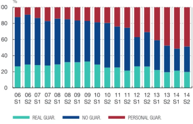
Figure 1 depicts the evolution of the proportion of the value of loans backed by personal and real guarantees, for a Spanish financial institution and its subsidiaries from the first semester of 2006 to the second semester of 2014. The figure shows that the outstanding loan amounts without explicit guarantees significantly decreased over time. It also reveals different patterns in the imposition of personal and real guarantees. While the amount collateralized through personal guarantees displays a significant increase, particularly after the second semester of 2011, the proportion corresponding to real guarantees remains stable. The increase of collateralized loans (of either guarantee type) may be related, on the one hand, to the need to mitigate credit risk in a context of uncertainty and weak global economic conditions. On the other hand, guarantees play a key role in capital regulation, where assets weighted by their risk level are fundamental.
The empirical literature so far has mainly focused on the determinants behind the use of real guarantees or collateral (e.g., Jiménez et al., 2006; Berger et al., 2011). Because of data limitations, less is known about the determinants of personal guarantees usage and, in general, about the differences between personal and real guarantees. In this paper, we break new ground by examining the determinants of the imposition of personal versus real guarantees, their use to improve bank loan
LOAN AMOUNT OUTSTANDING FIGURE 1
0 20 40 60 80 100 06 S1S20607S1 07S2S108 08S2S109 09S2S110 10S2 11S1S211S112 S21213S1S21314S1 14S2
REAL GUAR. NO GUAR. PERSONAL GUAR.
portfolio credit risk and capital ratios, and the implied costs and benefits for the firm. To address these questions, we use a unique and proprietary dataset of 477,209 loan contracts granted over the 2006-2014 period by a Spanish financial institution and its subsidiaries.
Different Drivers for Different Types of Guarantees
Our first research goal is to analyze whether the two types of guarantees are driven by different factors, by means of an OLS regression where the existence/ absence of personal or real guarantees (1/0) in a given loan contract i, denoted as Gi, is regressed on several sets of variables, relating to characteristics of the branch (distance between the bank branch and the headquarters), of the loan (maturity and size), of the firm (total assets, leverage, return on assets (ROA) and a refinancing dummy) and of the bank/ subsidiary-firm pair (a dummy based on existence of additional outstanding contracts between the parent bank or a subsidiary and the firm). The regression also includes fixed effects for each sector, bank/subsidiary, year, and province:
Gi = α + β1 BBo + β2 Li + β3 BFb,f,t + β4 Ff,t + θs + μb + γy + δp + εi (1) Here BBo, Li, BFb,f,t and Ff,t stand for branch, loan, bank/ subsidiary-firm, and firm characteristics, respectively. Both bank/subsidiary-firm and firm characteristics refer to the month before the loan is granted (t). The subscript b denotes the bank/subsidiary granting the loan in branch o to firm f operating in sector s and located in province p. The subscript y denotes the year in which the loan is granted and so, the term γy refers to the use of year fixed effects. Standard errors are clustered at the firm level.
The resulting coefficients on loan maturity are positive and significant for both personal and real guarantees. This is in agreement with previous literature (see Boot et al. (1991) among others) which showed that for longer-maturity loans, banks are more likely to request collateral, to align the incentives of the borrower and the lender. However, this effect is larger in economic terms in the case of real collateral, supporting the idea that as loans become longer-term, e.g., mortgages, the bank relies more on tangible real assets than on personal guarantees, which may be more uncertain since they depend on the firm’s manager’s present and future wealth. For the same reason, in the presence of large loans, the bank may prefer to request real collateral to seize the real assets in case of default.
The moral hazard literature documents that when lenders can observe a borrower’s credit quality, low-quality borrowers obtain loans with collateral while high-quality borrowers obtain loans without having to pledge collateral (Boot et al., 1991; Berger and Udell, 1990 and 1995; and Jiménez et al, 2006). In line with this theory, we document that overall, firm characteristics suggesting higher creditworthiness imply lower guarantees requirements. Moreover, we document that banks prefer personal guarantees when the economic conditions of the firm and/or the overall economy deteriorate, perhaps because personal guarantees are the ones with the strongest effects on incentives (Voordeckers and Steijvers, 2006).
In view of these results and the explanatory power associated to each group of variables, we conclude that real guarantees are mostly driven by loan characteristics, whereas personal guarantees are mostly driven by overall economic conditions. Indeed, the year fixed-effects coefficients (γy ) increase sharply after 2011 for the case of personal guarantees. This effect could be driven by the Spanish economic and financial crisis, or by requirements that European banks improve their capital ratios – we further elaborate on this point in the next section.
What Changed After 2011 in Guarantee Requirements?
Figure 1 reveals a noteworthy change of strategy with regard to guarantees requirements in 2011. Concretely, after October 2011 there is a sharp increase in the requirement of personal guarantees. This is the outcome of a combination of two events: i) recommendations and measures following the July 2011 stress test results in an environment of weak economic conditions; and ii) the EU agreement in October 2011 that required European banks to increase their capital buffers.
Both events help explain the increasing demand for guarantees since these represent a natural mechanism to limit losses and to align the interests of creditors and debtors by mitigating default rates. Moreover, effective guarantees (i.e., guarantees that fulfill certain regulatory criteria) might contribute to improved capital ratios by reducing risk-weighted assets (RWA). In fact, the European Banking Authority (EBA) highlights the usefulness of improvements in collateral and guarantees as a mitigating measure to reduce RWA. In this context, it is relevant to investigate the factors behind banks’ use of each type of guarantee from 2011 onwards.
One factor favoring personal guarantees is their role as a discipline device to limit the borrowers’ incentives to take risks, more effectively than business collateral (Mann, 1997). Moreover, personal guarantees could be more valuable than real guarantees if the guarantor’s personal assets are easier to value or sell, compared to certain firm-specific assets or human capital (Bodenhorn, 2003). Another reason to use personal guarantees is their potential efficiency advantage for the bank: personal guarantees can be rapidly and efficiently executed through extrajudicial enforcement. Finally, personal guarantees could also be of interest for banks to reduce their RWA. All of these incentives suggest that personal guarantees will be preferred to real guarantees in the post-October 2011 context. To test this hypothesis, we estimate equation (1) using a 3-month window before and after October 2011 on the same set of explanatory variables with the exception of the year fixed effects.1 We include a dummy for the policy change that takes the value one after October 2011, and equals zero otherwise.
We find that the use of personal and real guarantees is significantly more widespread after the bank guarantee policy change, with personal guarantees increasing substantially more. In fact, half of the variation in the use of personal guarantees is explained by this policy change. Results for real guarantees stand in stark contrast, as the policy change only explains around three percent. One may argue that if the bank uses guarantees to improve its regulatory capital, better capitalized subsidiaries should require guarantees less frequently. We take advantage of information about the specific bank/subsidiary granting the loan to conduct a formal test on this issue. To that end, we supplement equation (1) with a dummy variable that equals one if the total capital ratio of the bank/subsidiary granting the loan is above the median across the bank and its subsidiaries, and its interaction with the policy change dummy (the dummy equals one after October 2011).2 We document that credit institutions with a better capital position make less use of both real and personal guarantees. The lower use of guarantees by better capitalized subsidiaries is even more evident in the case of personal guarantees after October 2011, confirming the idea that the policy change affected those subsidiaries with lower capital ratios.
Guarantees, Firms’ Risk-Taking and Performance
We finally analyze whether guarantees lead to lower default rates and higher firm profitability, with a special focus on the post-October 2011 period.
A common result in the scarce literature analyzing the performance of firms that take out secured loans is that collateralized loans exhibit higher default probabilities because borrowers that pledge collateral are riskier ex-ante (Jiménez and Saurina, 2004; and Berger et al., 2011). However, Berger et al. (2016) show that the effect of collateral on ex-post performance could depend on the specific type of collateral. Thus, they find that liquid collateral has stronger risk-reducing incentives.
Our setting allows us to analyze in detail the risk and performance profiles of firms depending on whether the lender requires personal or real guarantees. We first analyze firms’ risk-taking, as measured by a dummy variable that takes the value of one if a firm defaults on its loan within a year after the first time it pledged guarantees, conditioned on not having defaulted prior to that event. Those individual firms that pledged guarantees for the first time in a given loan contract (treatment group) are then matched to a control group. This group consists of firms in the same industry, with similar size and profitability that got the loan the same year as the corresponding firm in the treatment group but did not pledge guarantees after the granting of the loan and did not pledge guarantees in the prior three years. The indicator of default for each firm in excess of the average indicator in the corresponding control group is then regressed on a constant. The resulting coefficient represents the probability of a loan default for those firms that pledged guarantees (treatment group) for the first time (i.e., we exclude repeat uses of guarantees) in excess of the average probability of default of the corresponding control group. We perform two regression analyses for the two types of guarantees using two different time periods corresponding to the year in which the loans were granted: 2006-2010 and 2012-2013.
Besides studying default, we also perform a similar analysis, using the same treatment and control groups, to study the effect of guarantees on firms’ performance. The dependent variable in the new analysis is the firm’s excess ROA, which is defined as its ROA a year after the firm pledged guarantees for the first time in excess of the ROA of the control group. The control group consists of firms in the same industry with similar size,
1 We add to the specification a proxy for overall economic risk, as measured by the 5-year sovereign CDS spread.
2 The bank/subsidiary fixed effects used in the baseline regression are excluded from this specification.
profitability, and risk profile that got the loan the same year as the corresponding firm in the treatment group but did not pledge guarantees to obtain the loan. Results show that for those loans granted during the period 2006-2010, personal guarantees were associated with a significant reduction in firm risk whereas the effect of real guarantees is not statistically different from zero. In fact, the economic effect, obtained as the estimated coefficient for the treatment group relative to the average default probability of the treatment group before the event, is sizeable in the case of personal guarantees, i.e.,–9.5%. Personal guarantees could have led managers to increase their effort level and to lower their risk-appetite to avoid losing their pledged personal wealth in case of default. Moreover, the beneficial effect of personal guarantees on loan default probabilities is not associated with a decrease in firms’ performance.
However, when analyzing loans granted in 2012-2013, personal guarantees are not associated with a significant reduction in risk-taking. The extensive use of personal guarantees in the second sub-period might have led to less selective decisions on the firms pledging guarantees, if they were used for regulatory capital purposes rather than to discipline borrowers. Thus, after the extensive use of this type of guarantees and the substantial increase in their coverage ratio,3 the borrowers’ incentive to take any risk could be so low that it could discourage firms to undertake certain investments, affecting the efficiency of their investment decisions. This could explain the negative effect found in our paper on firm performance, and, as a consequence, on the real economy.
The strategy adopted after 2011 may be positive in terms of financial stability since it implies that banks can better hedge potential defaults and improve capital ratios. Nevertheless, the use of personal guarantees with a higher coverage ratio implies that the risk ultimately affects the incentives of firms’ managers and
this could penalize the effectiveness of their decisions and their current and future enterprises. This result highlights that guarantees can also have costs, which are associated to their overuse.
REFERENCES
BERGER, A. N., W. S. FRAME and V. IOANNIDOU (2011). Tests of ex ante versus ex post theories of collateral using private and public information. Journal of Financial Economics 100, pp. 85-97. BERGER, A. N., W. S. FRAME and V. IOANNIDOU
(2016). Reexamining the empirical relation between loan risk and collateral: The roles of collateral liquidity and types. Journal of Financial Intermediation, 26, pp. 28-46.
BERGER, A. N., and G. F. UDELL (1990). Collateral, loan quality, and bank risk. Journal of Monetary Economics 25, pp. 21–42.
BERGER, A. N., and G. F. UDELL (1995). Relationship lending and lines of credit in small firm finance. Journal of Business 68, pp. 351–382.
BODENHORN, H. (2003). Short-term loans and long-term relationships: Relationship lending in early America. Journal of Money, Credit and Banking 35, pp. 485–505.
BOOT, A. W. A., A.V. THAKOR and G. F. UDELL (1991). Secured lending and default risk: equilibrium analysis, policy implications and empirical results. Economic Journal 101, pp. 458–472.
JIMÉNEZ, G., V. SALAS and J. SAURINA (2006). Determinants of collateral. Journal of Financial Economics 81, pp. 255-281.
JIMÉNEZ, G., and J. SAURINA (2004). Collateral, type of lender and relationship banking as determinants of credit risk. Journal of Banking and Finance, 28, pp. 2191-2212.
MANN, R.J. (1997). The role of secured credit in small-business lending, The Georgetown Law Journal 86, pp. 1–44.
VOORDECKERS, W., and T. STEIJVERS (2006). Business collateral and personal commitments in SME lending, Journal of Banking and Finance 30, 3067–3086.
3 The coverage ratio is obtained as the proportion of the loan size that is hedged by the guarantee associated with that risk.
MAKING ROOM FOR THE NEEDY: THE CREDIT-REALLOCATION EFFECTS OF THE ECB’S CORPORATE QE
ÓSCAR ARCE, RICARDO GIMENO AND SERGIO MAYORDOMO
WORKING PAPER 1743
We analyse how the European Central Bank’s purchases of corporate bonds under its Corporate Sector Purchase Programme (CSPP) affected the financing of Spanish non-financial firms. We first document that the announcement of the CSPP in March 2016 significantly raised these firms’ propensity to issue CSPP-eligible bonds. The flipside was a drop in the demand for bank loans by these firms. Moreover, the drop in credit given to bond-issuers, which are usually large corporations, unchained a positive and significant side effect on the flow of new loans extended to firms, typically smaller, that do not issue bonds. Specifically, we find that around 78% of the drop in loans previously given to bond issuers was redirected to other companies, which, in turn, raised their level of investment. The previous reallocation of credit was amplified by the ECB’s Targeted Longer Term Refinancing Operations (TLTRO).
1 Introduction
The Governing Council of the European Central Bank (ECB) announced in March 2016 the launch of a corporate sector purchase programme (CSPP) as an additional leg of its quantitative easing programme, known as the Asset Purchase Programme (APP). Under the CSPP, the Eurosystem buys debt securities issued by euro area non-financial corporations, with the goal of improving the pass-through of its monetary policy to the real economy. By October 2016, the market value of outstanding bonds eligible under the CSPP amounted to near 320 billion euros, and the Eurosystem had already purchased almost 12% of them.
In this paper, we analyse how the CSPP changed the financing conditions and the external financing mix of Spanish non-financial corporations. In addition to the direct effects on firms issuing eligible bonds, we study the existence of potential side effects of the central bank’s programme on the financing conditions of firms not issuing CSPP-eligible claims. The side effects or spillovers we look at operate through the reallocation of the supply of bank loans from firms issuing CSPP-eligible paper to companies that do not raise funding in the capital markets by issuing bonds, which are typically smaller than the issuers of CSPP-eligible bonds.
2
Direct effects of the CSPP
2.1 Cost of issuance
From the announcement of the CSPP in March 2016 until mid-April, the average yield of eligible bonds issued by Spanish non-financial corporations decreased by 44 basis points (bp); see Figure 1. This decline represents 30% of the average yield during that period. The impact on eligible bond yields around the initiation of the CSPP purchases, in June 2016, was more modest, which suggests that the effect of the programme may already have been factored into bond prices by that time. Interestingly, the effect of the programme was not limited to CSPP-eligible securities, but also extended to others, in particular, to bonds issued by non-financial corporations with credit ratings below investment grade (high-yield bonds).
The results of an econometric analysis show that the average yield of eligible bonds dropped 46 bp more than the overnight indexed swap (OIS) rate from the announcement of the program to the date when the purchases began. From then until the end of the sample (July 2016) the excess yield of the eligible bonds continued decreased further, but by a smaller amount (7.6 bp).1 0 1 2 3 4 5 6 0.0 0.4 0.8 1.2 1.6 2.0 2.4
Jan. Feb. Mar. Apr. May. Jun. Jul. Aug. Sep. Oct.
PUBLIC DEBT (5-10 YEARS AVERAGE) FINANCIAL CORPORATIONS. INVESTMENT GRADE NON-FINANCIAL CORPORATIONS. INVESTMENT GRADE NON-FINANCIAL CORPORATIONS. HIGH YIELD (RIGHT-HAND SCALE)
CSPP Announcement
Purchases start-date AVERAGE YIELD OF SPANISH LONG-TERM DEBT SECURITY ISSUES (%)
FIGURE 1
1 The end of the sample period is determinated by data availability on specific bond purchases.
2.2 Bond issuance activity
Beyond the effects of CSPP on yields, we also show that groups issuing CSPP-eligible bonds raised their volume of new issuances following the launch of the programme.2 Concretely, we find that the announcement of the CSPP pushed up by almost one third the probability that groups issuing eligible bonds increased their issuances. The effect of the programme was not limited to CSPP-eligible securities, but also extended, although to a lesser extent, to other bonds. Specifically, the probability that groups with non-eligible bonds increased their issuances rose by 6% in the quarter following the date of announcement.
We are also interested in knowing whether the funds obtained from the newly issued bonds under the CSPP served as a substitute for bank loans. To this end, we run a regression analysis in which the credit growth rate of a given group with a given bank between February 2016 and June 2016 is regressed on the group’s net growth of bonds outstanding during the quarter following the announcement of the CSPP, and a set of control variables at group and group-bank level. The results show that for each 1% increase in the net amount of bonds outstanding in the quarter following the CSPP announcement, the credit balance of groups diminished, on average, by around 0.44%. Hence, parallel to the increase in issuance activity, there was a substantial decrease in the credit exposure of resident credit institutions to the bond-issuing companies, as measured relative to total assets (see Figure 2).
3 Indirect effects of the CSPP
3.1 The credit reallocation channel
Against the previous contraction in the demand for loans by large bond-issuing corporates, we next analyze the role of the CSPP in promoting a reallocation of credit to non-bond issuing firms. To this aim, we use a regression analysis in which the dependent variable is the increase in the credit balance of firm j at bankb one month before the announcement of the CSPP (February 2016) and one quarter afterwards (June 2016), divided by the average credit balance in both periods (Creditj, b ). The main explanatory variables are the ratio of total credit outflows from bond issuers relative to bank b total assets during the time window mentioned above (Outflows/TA b ), and the interaction of the previous variable with two dummy variables related to the size of firmj that denote whether it is a medium-sized (D.Median j ) or micro-small
(D.Small j ) firm. In addition, we include some variables related to the characteristics of the bank and the firm:
Creditj, b= α + β1 Outflows/TA b + β2 D.Median j + β3 D.Small j + β4 D.Median j x Outflows/TA b + β5 D.Small j x Outflows/TA b + δF j + γBb+ θFB jb + ε j, b (1) Here, the coefficient β1 can be interpreted as the percentage change in credit granted to non-issuing large firms one quarter after the announcement of the CSPP, given an outflow of 1% in the credit balance of firms that are bond issuers. The sum of coefficients β1 and β4 (β1 and
β5 ) can be interpreted as the change in credit to medium-sized (micro/small) firms after the announcement of the CSPP given the same 1% outflow in the credit balance of bond issuers. Firm variables, represented by Fj , include profitability and risk. Bb denotes a set of bank characteristics such as bank size, profitability, financial strength, risk profile, percentage of liquid assets over total assets, and business model. Our sample consists of 29 resident credit institutions including commercial banks, saving banks and credit cooperatives, and 303,915 Spanish non-financial corporations j that do not issue bonds. Finally, we include joint firm-bank characteristics, such as the length of the bank-firm relationship immediately before the CSPP announcement. The information on loans is obtained from the Banco de España’s Central Credit Register (CCR). We aggregate the outstanding amount of credit of each firm in each bank at a monthly basis to obtain total credit (both drawn and undrawn in the case of credit lines). The CCR is
2 We consider groups instead of firms in this analysis because domestic and foreign subsidiaries are responsible for an important fraction of groups’ bond issuances.
1.60% 1.80% 2.00% 2.20% 2.40% 1.00% 1.10% 1.20% 1.30% 1.40%
AVERAGE WEIGHTED AVERAGE (RIGHT AXIS)
Credit Exposure / TA (%) CSPP Announcement
2015.06 2015.09 2015.12 2016.03 2016.06 2016.09 2016.12
RELATIVE CREDIT EXPOSURE OF RESIDENT CREDIT INSTITUTIONS (OVER TOTAL ASSETS) TO DEBT ISSUER GROUPS AROUND
AND AFTER ANNOUNCEMENT OF THE CSPP
These operations were conducted once a quarter between June 2016 and March 2017. Under TLTRO-II, banks were able to borrow a total amount of up to 30% of the eligible part of their outstanding loans as of 31 January 2016, net of any amount previously borrowed under the previous TLTRO-I scheme and still outstanding at the time of the settlement of TLTRO II.
Banks were given the opportunity to repay funds borrowed under TLTRO-I early, and switch to TLTRO-II funds. In fact, as detailed in ECB (2017), the vast majority of these funds were transferred to the TLTRO-II scheme. This shift of funds between the two TLTRO programmes was attractive because the second programme lengthened the maturity of funding provided by the ECB and lowered its cost. In particular, counterparties will receive a maximum rate reduction equal to the difference between the main refinancing operations (MRO) rate prevailing at the time of allotment (which is 0% since March 2016) and the rate on the deposit facility (which stood at –0.4%) applicable at the time of take-up if they exceed their benchmark stock of eligible loans by 2.5% in total as of 31 January 2018.
The previous pricing scheme implies that the decrease in lending given to bond issuers after the announcement of the CSPP could have an impact on the effective borrowing rate for those banks that were financing themselves through the TLTRO and, hence, on their lending incentives. To explore this possibility, we investigate empirically whether banks relying more on TLTRO increased their lending to non-issuing firms to a higher extent than banks less dependent on TLTRO funding, for a given decrease in the flow of loans to issuing firms after the CSPP. Considering two hypothetical banks that have both experienced high credit outflows from bond issuers, one of which has used up 50% of its TLTRO limit, while the other has not taken up TLTRO funds, we find that the former bank would increase its credit to a given firm on average by 15% after the announcement of the CSPP, whereas in the latter case this increase would be just 7%. Hence, the reallocation of credit documented above was amplified by the ECB’s TLTRO-II.
REFERENCES
EUROPEAN CENTRAL BANK (2016). Decision (EU) 2016/948 of the European Central Bank, 1 June 2016 on the implementation of the corporate sector purchase programme (ECB/2016/16).
EUROPEAN CENTRAL BANK (2017). The targeted longer-term refinancing operations: and overview of the take-up and their impact on bank intermediation, Box 5, Economic Bulletin, No 3/2017.
merged with a second dataset, the Integrated Central Balance Sheet Data Office Survey (CBI), which includes information from firms’ accounts filed with the mercantile registries. The CBI dataset enables us to classify the firms as micro/small or medium-sized firms according to the European Commission criteria.
The estimation of equation (1) reveals that banks that suffered a more severe reduction in credit demand from large bond-issuing companies increased their loans to large companies that did not issue bonds as detailed above, but also, although to a lesser extent, to medium-sized and micro/small firms. After controlling for bank and firm characteristics, we find that a drop of one euro in the credit balance of bond issuer groups led to an average increase of around 78 euro cents in the credit balance of firms that do not issue bonds one quarter after the announcement of the CSPP. In particular, the increase in the average credit balance was worth 48, 15, and 15 euro cents in the case of large, medium-sized and small firms. This represents 3.3%, 1.8%, and 0.8% of the firms’ average credit balances before the CSPP announcement, respectively. Furthermore, the reallocation of credit towards non-issuing firms led to an increase in the investment of these firms.
Banks differentiate between large, medium-sized, and small firms probably because the latter are riskier and could lead to higher expected costs of absorbing potential losses. Thus, the cascade effect along the firm-size dimension derived from the substitution of bank loans by bonds by regular issuers could reflect the banks’ attempt to preserve their risk profile to the extent possible. This conjecture is supported by the fact that banks suffering credit outflows from bond issuers mainly raised their flow of credit towards large and medium-sized firms, which are relatively safer borrowers than micro/small firms. Based on this conjecture, we extend the previous econometric analysis by splitting firms according to their risk instead of their size, and confirm that banks suffering credit outflows from bond issuers exhibit a strong preference for safer borrowers. Hence, minimizing the change in the risk profile of their loan portfolios appears to have been a central motive behind the profile of lending in this credit-cascade process.
3.2 The amplifying effect of the TLTRO on the
credit reallocation channel
The ECB’s CSPP programme overlapped with other unconventional monetary policy measures, including its Targeted Longer Term Refinancing Operations (TLTRO). The first phase of TLTRO was followed by a second series of four operations (TLTRO-II), announced on March 2016, coinciding with the CSPP announcement.