A note on using the collocation method for modelling the dynamics of a flexible continuous beam subject to impacts

This is a repository copy of A note on using the collocation method for modelling the dynamics of a flexible continuous beam subject to impacts.

White Rose Research Online URL for this paper: http://eprints.whiterose.ac.uk/79683/

Article:

Wagg, D.J. (2004) A note on using the collocation method for modelling the dynamics of a flexible continuous beam subject to impacts. Journal of Sound and Vibration, 276 (3-5). 1128 - 1134. ISSN 1541-0161

https://doi.org/10.1016/j.jsv.2003.11.039

Reuse

Unless indicated otherwise, fulltext items are protected by copyright with all rights reserved. The copyright exception in section 29 of the Copyright, Designs and Patents Act 1988 allows the making of a single copy solely for the purpose of non-commercial research or private study within the limits of fair dealing. The publisher or other rights-holder may allow further reproduction and re-use of this version - refer to the White Rose Research Online record for this item. Where records identify the publisher as the copyright holder, users can verify any specific terms of use on the publisher’s website.

Takedown

If you consider content in White Rose Research Online to be in breach of UK law, please notify us by

A note on using the collocation method for

modelling the dynamics of a flexible

continuous beam subject to impacts

D. J. Wagg

Department of Mechanical Engineering, University of Bristol, Queens Building, University Walk, Bristol BS8 1TR, U.K.

Fax:0117 9294423

Key words: Collocation, Euler-Bernoulli beam, vibro-impact

15 pages, 4 Figures.

1 Introduction

The use of nonsmooth modelling techniques to model the dynamics of a flexible

impacting beam has recently been reported by [1]. The method used was based

on taking a Galerkin approximation [2] of the partial differential equation

(PDE) governing the dynamics of the beam away from impact, and coupling

this to a nonsmooth coefficient of restitution rule to model the impact [3]. In

this letter the advantages and limitations of using a collocation method instead

of the Galerkin method combined with a nonsmooth impact law are discussed.

Journal of Sound and Vibration 276 (2004) 1128–1134

The example of a flexible beam subject to a motion limiting constraint is used,

similar to that discussed in [1].

The general problem of a cantilever beam impacting against an impact stop

has been considered by several authors — see for example [4–7]. The

colloca-tion approach has been used for modelling a variety of engineering problems —

see for example [8–11]. In this example, collocation has the advantage that

un-like the Galerkin method there is no requirement to integrate the mode shape

over the domain of interest in order to decouple the system modal equations.

This means that (in general) the collocation method can be applied to a larger

range of problems, particularly those with more complex geometry. There is a

further advantage in that the Galerkin approach [1] required the exact solution

for the modal equations between impact, whereas with this collocation method

a numerical integration routine is used. However, we note that in general it is

not necessary to use exact solutions for the trial functions when applying the

Galerkin method.

For piecewise-linear systems, Wang & Wang [12] describe a collocation method

for simulating periodic responses. The use of collocation methods for modelling

periodic motions in constrained multi-body systems has also been considered

by Franke & F¨uhrer [13]. In the approach described here there is no a priori

requirement for periodicity.

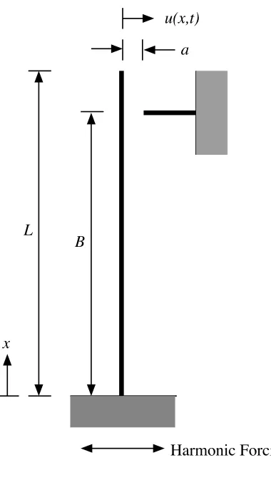
2 Mathematical model

The system considered is a clamped cantilever beam with a motion limiting

is positioned at a distance B from the base along the beam, and with an

initial transverse distance a from the beam which is harmonically forced at

its base. The transverse vibration of the centre line of the beam is denoted

by u(x, t), where x is the length along the beam from the base andt is time.

Away from the impact constraint, the beam is assumed to be governed by the

Euler-Bernoulli equation with damping and external forcing

EI∂

4

u ∂x4 +η

∂u ∂t +ρA

∂2

u

∂t2 =f(x, t) u < a. (1)

whereE is the Young’s modulus,ρdensity,Across-sectional area,ηthe

damp-ing constant and I the second moment of area for the beam of length L.

When an impact occurs,u(B, t) =aand a coefficient of restitution rule of the

form

˙

u(B, t+) =−ru˙(B, t−) u(B, t−) =a, (2)

is applied, where t− is the time just before impact, t+ is the time just after

impact and r ∈ [0,1] is the coefficient of restitution. It is assumed that the

velocities are normal to the beam centre line, and that the tangential velocity

component at impact is negligible. Equation (2) is applied instantaneously

such thatt− =t+, and a nonsmooth discontinuity in velocity occurs at impact.

However, for a continuous structural element, such as a beam, the velocity is

a continuous function of beam length. Thus, in order to apply the nonsmooth

impact condition, equation (2), at u = a, the velocity components for the

non-impacting part of the beam x6=B remain unaffected such that

˙

Journal of Sound and Vibration 276 (2004) 1128–1134

applies. The combination of equations (2) and (3) are essentially a nonsmooth

representation of the physical impact process for the beam. In the physical

beam system the contact time will be finite (though small for materials with

high stiffness) and the velocity reversal will propagate outwards from the point

of impact, a process which is captured with this type of model.

It is now assumed that there is a series solution to the Euler-Bernoulli equation

given by

u(x, t) =

∞ X

j=1

φj(x)qj(t), (4)

whereφj(s) are the normal mode shapes of the beam, andqj(t) are the modal

coordinates [14]. Then substituting equation (4), into the Euler-Bernoulli

equation (equation (1)) gives

N

X

j=1

φjq¨j(t) +βφjq˙j(t) +αφ

′′′′

j qj(t)

=γf(x, t) j = 1,2,3. . . N, (5)

where ()′

represents differentiation with respect tox, an overdot differentiation

with respect tot,α=EI/ρA,β =η/ρA andγ = 1/ρA. As the normal linear

beam modes are being used for this example, the standard relationship that

φ′′′′

j =ξ 4

jφj, where

ξ4 j =ω

2 nj

ρAL4

EI (6)

and ωnj is the jth natural frequency [15] will be used. In the case when this

doesn’t hold, collocation can still be applied providing the fourth derivative of

equation (6) into equation (5) gives

N

X

j=1

φjq¨j(t) +βφjq˙j(t) +αξ 4

jφjqj(t)

=γf(x, t) j = 1,2,3. . . N. (7)

N collocation points x1, x2, . . . , xN are now chosen along the length of the

beam. Collocation points are usually chosen at evenly spaced intervals, and a

key requirement for this method is that the point of contact, x = B, is at a

collocation point. Now for the N discrete collocation points equation (7) can

be represented in a matrix form

Φ¨q+βΦ ˙q+αΦˆξq =γF (8)

where                    

φ1(x1) φ2(x1) . . . φN(x1)

φ1(x2) φ2(x2) . . . φN(x2)

... ... . . . ...

φ1(xN) φ2(xN). . . φN(xN)

                    , (9)

q= [q1, q2. . . qN]T, ˆξ =diag{ξ14, ξ 4 2. . . ξ

4

N}andF = [f(x1, t), f(x2, t). . . , f(xN, t)]T.

Multiplying equation (8) by Φ−1

and putting it into first order form gives

˙

Journal of Sound and Vibration 276 (2004) 1128–1134 where z= [q,q˙]T_{, ˆF = [0}

N, γΦ−1F]T and

H =        

0N IN

−αξˆ−βIN

        . (11)

Equation (10) can now be integrated forward in time from a set of initial

conditions using a suitable time-stepping method — in this case a fourth

order Runge-Kutta method [16] is used.

To apply the nonsmooth impact condition, a coefficient of restitution matrix,R

is defined using equations (2) and (3). Equation (2) applies to the collocation

point where impact occurs, x = B, and equation (3) applies to all other

collocation points. For example, for a choice of N collocation points with the

impact at point N (the beam tip) the coefficient of restitution matrix is

R =                    

1 0 . . . 0

0 1 . . . 0

..

. ... . . . ...

0 0 . . .−r                     , (12)

At each time step the condition for the beam having an impact, u(B) > a,

is checked. Once an impact is detected a root finding method is used to find

the exact time at which u(B) = a. Then the modal velocities are updated

according to the matrix coefficient of restitution rule [1]

˙

q(t+) = [Φ]

−1

and time stepping begins again.

3 Example: four mode model of a cantilever beam

As an example a cantilever beam which has dimensions length 300mm width

25.5mm and thickness 0.49mm is considered. The properties of the beam are

taken as the following parameter values; Young’s ModulusE=205×109

N/m2

,

second moment of area I=24.4×10−14

m4

, density ρ=8500kg/m3

, cross

sec-tional areaA=12.4×10−6

m2

damping constantη=0.005Ns/m and lengthL=0.3m.

In this example N = 4 is selected and the initial conditions are chosen such

that all displacements and velocities of the beam are zero at time t = 0.

The forcing function is assumed to be separable into space and time

depen-dant functions such that f(x, t) = g(x)h(t), where for this example h(t) =

P cos(Ωt), P = 0.0006m and Ω = 28.3rads/sec. Evaluating the forcing

func-tions at the collocation points givesF = [g(x1), g(x2), . . . , g(xN)]Th(t) and for

this example g(xi) = 1 for i = 1, . . . , N, and it is assumed that the impact

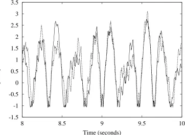
occurs at the beam tip B = L. Then 10 seconds of vibro-impact motion is

simulated and the last two seconds plotted, which is shown in Figure 2.

In Figure 2 the solid line represents the time series simulation computed

using the collocation method described in section 2. For a comparison the

nonsmooth-Galerkin method used in [1] is plotted as a dashed line. The two

methods give qualitatively similar responses in that the maximum amplitudes

and times of impacts are similar. The periodicity of the response is clearly

shown by both simulations.

Journal of Sound and Vibration 276 (2004) 1128–1134

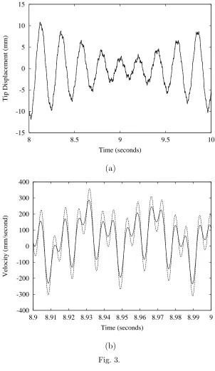
This is demonstrated more clearly when exactly the same simulation without

impacts is plotted — Figure 3. In Figure 3 (a), showing displacement, the

solid line and dashed line are indistinguishable, but in Figure 3 (b), showing a

short section of the velocity signal, there are significant differences between the

simulations. As a result when an impact occurs the nonsmooth jump in velocity

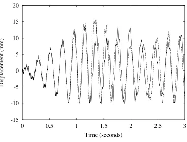
causes the post impact behaviour of the two simulations to differ slightly. As

more impacts occur this initially small difference is compounded and the higher

frequency behaviour of the two approaches diverge — demonstrated in Figure

4. Defining the parameter regimes where reasonable quantitative agreement

between the two methods occurs is an area of future study.

It is worth reiterating at this point that the Nonsmooth-Galerkin method

de-scribed by [1] uses the exact solutions of the decomposed normal mode

equa-tions between impacts, and requires integration of the normal mode shapes

across the length of the beam. In principle, the collocation approach can be

applied with neither of these requirements, and can therefore be applied to

a wider range of problems. The trade off is that there is a cumulative

reduc-tion in accuracy for the high frequency part of the simulareduc-tion. However, for

the examples considered here the qualitative behaviour of the system is still

captured by the collocation method.

References

[1] D. J. Wagg, S. R. Bishop, Application of nonsmooth modelling techniques to

the dynamics of a flexible impacting beam, Journal of Sound and Vibration

256 (5) (2002) 803–820.

Springer-Verlag, 1984.

[3] S. R. Bishop, M. G. Thompson, S. Foale, Prediction of period-1 impacts in a

driven beam, Proceedings of the Royal Society of London A 452 (1996) 2579–

2592.

[4] J. L. Escalona, J. Valverde, J. Mayo, Domingez, Reference motion in deformable

bodies under rigid body motion and vibration. part ii: evaluation of the

coefficient of restitution for impacts, Journal of Sound and Vibration 264 (5)

(2003) 1057–1072.

[5] I. Svensson, Dynamic response of a constrained axially loaded beam, Journal

of Sound and Vibration 252 (4) (2002) 739–749.

[6] A. Fathi, N. Popplewell, Improved approximations for a beam impacting a stop,

Journal of Sound and Vibration 170 (3) (1994) 365–375.

[7] J. Wang, J. Kim, New analysis method for a thin beam impacting against a

stop based on the full continuous model, Journal of Sound and Vibration 191 (5)

(1996) 809–823.

[8] J. Kouatchou, Comparison of time and spatial collocation methods for the heat

equation, Journal of Computational and Applied Mathematics 150 (2003) 129–

141.

[9] K.-Y. Lee, A. A. Renshaw, Stability analysis of parametrically excited systems

using spectral collocation, Journal of Sound & Vibration 258 (4) (2002) 725–

739.

[10] R. Baltensperger, J.-P. Berrut, The linear rational collocation method, Journal

of Computational and Applied Mathematics 134 (2001) 243–258.

[11] B. Li, A crank-nicolson orthogonal spline collocation method for vibration

Journal of Sound and Vibration 276 (2004) 1128–1134

[12] Y. Wang, Z. Wang, Periodic response of piecewise-linear oscillators using

trigonometric collocation, Journal of Sound and Vibration 177 (4) (1994) 573–

576.

[13] C. Franke, C. F¨uhrer, Collocation methods for the investigation of periodic

motions of constrained multibody systems, Multibody System Dynamics 5

(2001) 133–158.

[14] R. Vichnevetsky, Computer methods for partial differential equations, Prentice

Hall, 1981.

[15] R. D. Blevins, Formulas for natural frequency and mode shape, New York: Van

Nostrand Reinhold, 1979.

[16] W. H. Press, S. A. Teukolsky, W. T. Vettering, B. P. Flannery, Numerical

Figure Captions

• Figure 1: Schematic representation of the continuous vibro-impact cantilever

beam system.

• Figure 2: Impacting beam simulation; parameter valuesus =−1.05,N = 4,

F = 0.0006, Ω = 28.3, η = 0.005, r = 0.8. Solid line; collocation, dashed

line; Galerkin.

• Figure 3: Non-impacting beam simulation; parameter values N = 4, F =

0.0006, Ω = 28.3, η = 0.005. Solid line; collocation, dashed line; Galerkin.

(a) Displacement, (b) Velocity.

• Figure 4: Impacting beam simulation; parameter values us =−10.05, N =

4,F = 0.0006, Ω = 28.3,η = 0.005, r= 0.8. Solid line; collocation, dashed

Journal of Sound and Vibration 276 (2004) 1128–1134

x L

B

a u(x,t)

Harmonic Forcing

-1.5 -1 -0.5 0 0.5 1 1.5 2 2.5 3 3.5

8 8.5 9 9.5 10

Tip Displacement (mm)

Time (seconds)

Journal of Sound and Vibration 276 (2004) 1128–1134

-15 -10 -5 0 5 10 15

8 8.5 9 9.5 10

Tip Displacement (mm)

Time (seconds)

(a)

-400 -300 -200 -100 0 100 200 300 400

8.9 8.91 8.92 8.93 8.94 8.95 8.96 8.97 8.98 8.99 9

Velocity (mm/second)

Time (seconds)

(b)

-15 -10 -5 0 5 10 15 20

0 0.5 1 1.5 2 2.5 3

Displacement (mm)

Time (seconds)