Efficient protocols for private record linkage

(1)

Efficient Protocols for Private Record Linkage

Zikai Wen

*†

Changyu Dong

*

[email protected]

†_{College of Information Science and Technology} *_{Dept. of Computer and Information Sciences}

Beijing University of Chemical Technology University of Strathclyde

Beijing, China Glasgow, UK

ABSTRACT

Record linkage allows data from different sources to be integrated to facilitate data mining tasks. However, in many cases, records have to be linked by personally identifiable information. To prevent privacy breaches, ideally records should be linked in a private way such that no information other than the matching result is leaked in the process. In this paper, we present an exact Private Record Link-age (PRL) protocol and an approximate PRL protocol. The exact PRL protocol is based on Oblivious Bloom Intersection, which is an efficient private set intersection protocol. The approximate PRL protocol extends the exact PRL protocol by incorporating Locality Sensitive Hash functions. Both protocols are secure in the semi-honest model. We also report the evaluation results based on our C implementation of the protocols. The results show that our proto-cols are efficient and effective.

1. INTRODUCTION

Data is invaluable to organizations. Everyday, a large amount of data is generated, collected and stored. By analyzing the data, new knowledge can be discovered that will lead to improvement in pub-lic health, productivity for government agencies, and competitive edge for a commercial enterprise. However, often data is possessed by different entities separately, therefore needs to be integrated to facilitate data mining that is not feasible on a single database. To link two databases, record pairs are compared using a variety of fields and record comparison functions. The goal is to classify the record pairs into matches and non-matches.

Linking data may cause privacy concerns. When linking two databases from different sources, the data usually lacks unique en-tity identifiers. That means linking is often based on some

person-ally identifiable information. Sharing personal information across

multiple entities may cause a breach of privacy. Legally, it may also be prohibited by laws and regulations. For example, in the USA the Health Insurance Portability and Accountability Act (HIPPA) sets the standard for protecting health data, e.g. what kind of match-ing and analysis can be conducted with health data, and at what level of detail health data can be published. Similarly, in Europe, Data Protection Directive regulates the processing of personal data.

Permission to make digital or hard copies of all or part of this work for personal or classroom use is granted without fee provided that copies are not made or distributed for profit or commercial advantage and that copies bear this notice and the full citation on the first page. Copyrights for components of this work owned by others than ACM must be honored. Abstracting with credit is permitted. To copy otherwise, or republish, to post on servers or to redistribute to lists, requires prior specific permission and/or a fee. Request permissions from [email protected].

SAC’14March 24-28, 2014, Gyeongju, Korea.

Thus it is vital to ensure that whenever databases are linked across organizations, privacy of individuals is maintained.

Private Record Linkage (PRL) is the process of identifying records from multiple data sources that refer to the same individual, with-out revealing more information besides the matched records. More formally, assumingAandB are the data owners and each holds a databaseDA, DB respectively, for each recordRAi ∈ DA and RBj ∈DB, they want to decide whetherRiA∼=RjBwhere∼=is the

match relation defined by certain record comparison functions. In the process data privacy must be retained in the sense that no more information other than the linking result (RAi ∼=RBj orRAi 6∼=RBj)

should be leaked. PRL has many practical uses. For example, epi-demiological research often requires correlated demographics data with diseases to identify possible risk factors or targets for preven-tive medicine. However in many countries the data is held sep-arately by different registries, and often privacy concerns arise if such data is stored and linked at a central location. As a result, in the past a few years we have seen a lot of research work in this area.

There are three requirements for a PRL protocol:

• Privacy: As one of the goals of PRL is to maintain privacy, it must not allow additional information to be leaked from the linking process. The privacy guarantee must stand rigorous analysis.

• Effective: In case of exact match, the identified matches must be correct. In case of non-exact match, the quality of the identified matches must conform certain evaluation criteria. • Efficient: The database being linked can be very large,

there-fore the protocol needs to be efficient so the linking can be done in a reasonable amount of time.

Our Contributions:In this paper, we present two novel and

effi-cient PRL protocols. They are based on Oblivious Bloom Intersec-tion, an efficient and scalable Private Set Intersection protocol. The first protocol supports exact match. The second protocol is built on top of the exact match protocol and supports similarity-based ap-proximate match by incorporating Locality Sensitive Hashing. The protocols are secure in the semi-honest model. The protocols are very efficient and have linear complexity. We have built prototypes of the PRL protocols and evaluated the protocols in terms of effi-ciency and accuracy. We also compared our protocols with other protocols and the comparison shows that our protocols are much more efficient.

2. RELATED WORK

(2)

back to [8]. The protocol hashes the records and uses the hash values instead of the records for linking two databases. The proto-col however is subject to frequency attacks because hash functions are deterministic. Later exact PRL work includes various protocols that rely on private set intersection [1, 9, 14, 11, 6, 12].

Approximate PRL usually depends on some sort of similarity measures. If, according to the chosen similarity measure, the dis-tance between two record values is less than a certain threshold, then the two records are considered a match. Many approximate PRL protocol are three-party protocols, i.e. apart from the two parties who hold the data, there is also a trusted or semi-trusted party involved in the protocol. In [5] the two parties hash their at-tribute values to be compared, then the hash values are sent to a third party who compares the values blindly and finds values in the two sets that match. In [19] the two parties embed their values us-ing the SparseMap method. Then the embedded strus-ings are sent to a third party who determines the similarity. A third party can make protocol more efficient. However, in practice a trusted or semi-trusted third party may not always be available. In a strict two-party setting, [2] links records by securely computing edit distance of strings, [18] securely computes TF-IDF (term-frequency, inverse document frequency), [22] uses phonetic functions and commuta-tive encryption to link records, and [24] proposed a very efficient protocol that first converts records into vectors and then securely computes the distance between each pair of the records. A good survey of PRL protocols can be found in [23].

Our protocol uses Bloom filters. Previously, a protocol in [20] is also based on Bloom filters. However, our approach is quite differ-ent from that in [20]. Firstly, in [20] , each record needs a Bloom filter to store q-grams of the attribute values to be compared, while in our protocol, only one Bloom filter is required for the whole database. Secondly, in [20], a semi-trusted third party is needed, while in our protocol we do not need a third party. The protocol in [20] has also been shown to be insecure [15]. Our protocol is secure in the semi-honest model.

3. THE EXACT PRL PROTOCOL

In this section, we introduce the exact PRL protocol. Here ex-act means the match relation is defined by an equality relation on the attribute values being compared. The protocol follows the pri-vate set intersection approach and is an extension of the Oblivious Bloom Intersection (OBI) protocol [7].

3.1 Oblivious Bloom Intersection

Oblivious Bloom Intersection (OBI) [7] is an efficient and scal-able private set intersection protocol. A private set intersection pro-tocol is a propro-tocol between two parties,AandB. Each party has a private set as input. The goal of the protocol is thatAlearns the intersection of the two input sets, but nothing more aboutB’s set, andBlearns nothing. A PRL protocol can be built on top of a pri-vate set intersection protocol directly. However, previous pripri-vate set intersection protocols are not efficient enough to be used in real applications. This situation is changed by the recently proposed OBI protocol. The OBI protocol adapts a very different approach for computing set intersections. It is mainly based on efficient hash operations. Therefore it is significantly faster than previous private set intersection protocols. In addition, the protocol can also be par-allelized easily, which means performance can be further improved by parallelization. The protocol is secure in the semi-honest model and an enhanced version is secure in the malicious model. We refer the readers to [7] for more details regarding OBI. In the rest of this section we will show how to modify OBI and build an exact PRL protocol on top of it.

3.2 Bloom Filters and Garbled Bloom Filters

The OBI protocol relies on Bloom filters (BF) and garbled Bloom filters (GBF). Both BF and GBF are probabilistic data structures that encode set membership and allow queries without false nega-tive but may have negligible false posinega-tive. The two data structures are both sizemarrays that can encode a setS of at mostn ele-ments, and are associated with a set ofkindependent uniform hash functionsH={h0, ..., hk−1}such that eachhimaps elements to

index numbers over the range[0, m−1]uniformly. The main differ-ence between the two is that a Bloom filter is a bit array while a gar-bled Bloom filter is an array ofλ-bit strings. We will use the nota-tion in [7]: we use(m, n, k, H)-Bloom filter to denote a Bloom fil-ter paramefil-terized by(m, n, k, H),(m, n, k, H, λ)-Garbled Bloom filter to denote a garbled Bloom filter parameterized by(m, n, k, H, λ), useBFSorGBFSto denote a Bloom filter or a garbled Bloom

fil-ter that encodes the setS, and useBFS[i]orGBFS[i]to denote

the bit or string at indexiin the filter’s array.

The two data structures work in a similar way. For a Bloom filter, to insert an elementx ∈ S into the filter, the element is hashed using thekhash functions and setBFS[hi(x)] = 1. To check if an

itemyis inS,yis hashed by thekhash functions, and all locations

yhashes to are checked. If any of the bits at the locations is 0 ,yis not inS, otherwiseyisprobablyinS. For a garbled Bloom filter, to insert an elementx∈Sinto the filter,xis split intokshares using an XOR-based secret sharing scheme. The secret sharing scheme ensures that the element can only be recovered from the shares if all k shares are available. The elementxis hashed using thek

hash functions to getkindexes and the shares ofxare stored in the

GBFarray by the indexes, one share at each index. To check if an itemyis inS,yis hashed by thekhash functions, and all strings at locationsyhashes to are retrieved back and XORed together. if the result string is noty,yis not inS, otherwiseyisprobablyinS.

3.3 Modified Garbled Bloom Filter

The idea of the OBI protocol is thatA encodes its set into a Bloom filter andBencodes its set into a garbled Bloom filter, then they run an oblivious transfer protocol so thatAreceives a new garbled Bloom filter that encodes the set intersection andBgets nothing. The reason whyAuses a Bloom filter andBuses a gar-bled Bloom filter is because if both parties uses Bloom filters then the protocol is not secure, while if both parties uses garbled Bloom filters then the protocol cannot produce meaning results.

However this approach cannot be directly used in PRL. The orig-inal algorithm in [7] for building garbled Bloom filters is not suit-able and needs to be modified. Loosely speaking, the original al-gorithm allowsAto find a subset of its records that can be linked to records inB’s database, butAcannot find out for each of the records in the subset, which record inB’s database is linked to it. Let us elaborate it: for a database that hasnrecords, we assume each recordRihas a unique identifieridiand there is a functionf

such thatxi=f(Ri)is computable andxican be used for record

matching purpose. For example, xican be the concatenation of

some attribute values ofRi, or a hash value ofRi(or part ofRi).

We say a recordRA

i ∈ DAmatches another record RBj ∈ DB

ifxAi =x B

j. For two databasesDAandDB, an exact PRL

pro-tocol should return the following: {(idA

i, idBj) |xAi =xBj}, i.e.

all pairs of record IDs of matching records in the two databases. If we use OBI without any modification, thenAuses the set of all

xAi to generate a Bloom filter, andBuses the set of allxBj to

gen-erate a garbled Bloom filter. Then they run the oblivious transfer protocol so thatAobtains a garbled Bloom filter that encodes the intersection. After that,Acan query eachxAi against the

(3)

inter-section. For eachxA

i such that the query result is positive,Aonly

knows it is in the intersection and then there must be somexBj such

thatxA

i = xBj. In other words, at the end of the protocol,Acan

only output{xAi |x A

i =x

B

j}, but not{(id A i, id

B j)|x

A

i =x

B j}.

This is because the garbled Bloom filter generated by the original algorithm does not allow us to encode any record ID information. To fix the problem, we modified the algorithm and the new algo-rithm is shown in Algoalgo-rithm 1. Accordingly, the query algoalgo-rithm is modified and is shown in Algorithm 2.

Algorithm 1:BuildGBF(D, n, m, k, H, λ)

input : A setD,n, m, k, λ,H={h0, ...hk−1}

output: An(m, n, k, H, λ)-garbled Bloom filterGBFD

1 GBFD= newm-element array of bit strings; 2 fori= 0tom−1do

3 GBFD[i]=NULL; // NULL is the special symbol that means no value

4 end

// encodes(_{xi, idi})rather than just_xias in the original algorithm

5 for each(xi, idi)∈Ddo

6 emptySlot =−1, finalShare=idi; // idiis the value to be stored

7 forj=0tok-1do

8 z=hj(xi); // get an index by hashing_xi

9 ifGBFD[z]==NULLthen

10 ifemptySlot ==−1then

11 emptySlot=z; // reserve this location for finalShare

12 else

13 GBFD[z]← {r 0,1}λ_; _//

generate a new share

14 finalShare=finalShare⊕GBFD[z];

15 end

16 else

17 finalShare=finalShare⊕GBFD[z]; // reuse a share

18 end

19 end

20 GBFS[emptySlot]=finalShare; // store the last share

21 end

22 fori= 0tom−1do

23 ifGBFD[i]==NULLthen

24 GBFD[i]← {r 0,1}λ_;

25 end

26 end

Algorithm 1 differs from the original algorithm only in one place: for each record, we split its identifieridi, rather thanxi, intok

shares on the fly and store the shares inGBFD[hj(xi)] (line

5-21). The intuition is that later the GBF query returns two things: (1) for eachxiwhetherxiis encoded in the GBF; (2) for eachxi

that is encoded in the GBF, the identifieridiof the recordRisuch

thatxi =f(Ri). Thus whenAqueries the intersection GBF, for

eachxA

i = xBj, it also gets the identifieridBj of the record from

whichxBj is extracted. SinceAknows the identifier of its record

from whichxA

i is extracted, nowAcan output(idAi, idBj).

Algorithm 2:QueryGBF(GBFD, x, k, H)

input : A garbled Bloom filterGBFD, an elementx,k,H={h0, ...hk−1}

output: the identifier ofRifor someRi∈Difx=f(Ri), NULL otherwise

1 recovered={0}λ_; 2 forj=0tok-1do

3 z=hj(x);

4 recovered=recovered⊕GBFD[z]; 5 end

// We assume that identifiers can be distinguished from random strings.

6 ifrecoveredis an identifierthen

7 returnrecovered; 8 else

9 return NULL; 10 end

3.4 PRL by Oblivious Bloom Intersection

The idea of the protocol is to compute and transfer a GBF that contains only the matching record identifiers toAin an oblivious way. The protocol runs as follows:

1. A’s private input isDA,B’s private input isDB. The

aux-iliary inputs include the security parameterλ, the maximum database sizen, the Bloom filter parametersm, kandH =

{h0, ..., hk−1}. The parameterkis set to be the same as the

security parameterλto make false positive negligible. 2. Agenerates an(m, n, k, H)-BF that encodes its records in

DA. To do so,Afirst produces an empty setSA, thenA

com-putes for eachRAi ∈ DA,xAi =f(RiA)and putsxAi into SA. ThenAencodesSAinto an(m, n, k, H)-BFBFSA.

3. Bgenerates an(m, n, k, H, λ)-GBF that encodes its records inDB. To do so,B first produces an empty setSB, then B computes for eachRiB ∈ DB, xBi = f(RBi)and puts

(xB

i , idBi)intoSB. ThenBencodesSBinto an(m, n, k, H, λ)

-GBFGBFSBusing Algorithm 1.

4. Auses its Bloom filter as the selection string and acts as the receiver in anOTm

λ protocol.Bacts as the sender in the OT

protocol to sendmpairs ofλ-bit strings(xi,0, xi,1)where xi,0is a uniformly random string andxi,1isGBFSB[i]. For 0≤i≤m−1, ifBFSA[i]is 0, thenAreceives a random

string, ifBFSA[i]is 1 it receivesGBFSB[i]. The result is

GBFmatch.

5. Afinds the matches by querying all elements inSAagainst GBFmatch.

At the end of step 4, A receives a new garbled Bloom filter

GBFmatch. This GBF encodes only identifiers of records inDB

that match records in DA. Let’s see why this is the case: for

any matching record pair(RA

i, RBj), we havexAi = xBj where

xA

i =f(RAi)andxBj =f(RBj). Note thatAandBuse the same

set of hash functionsHwhen buildingBFSAandGBFSBand the

hash functions are deterministic. Therefore, becausexA i = xBj,

for anyhl ∈ H we havezl = hl(xiA) = hl(xBj). InGBFSB,

eachGBFSB[zl]is a share ofid

B

j and it will be transferred toA

because BFSA[zl] = 1. So all shares ofid

B

j will be preserved

inGBFmatch and by queryingGBFmatch, Acan recoveridBj.

For any non-matching record pair(RA

i, RBj), sincexAi 6=xBj, we

have with a high probabilityhl(xAi)=6 hl(xBj), therefore with an

overwhelming probability, at least one share of idBj will not be

transferred toA. Instead, a random string will be transferred. Then whenAqueriesGBFmatch,idBj cannot be recovered because at

least one share is missing.

This protocol is secure in the semi-honest model [10]. We have the following theorem:

THEOREM 1. Letf≡be the exact record linkage function

de-fined as:f≡(DA, DB) = ({(idAi, id

B j)|x

A i =x

B

j},Λ), whereΛ

denotes the empty string. If OBI is secure in the semi-honest model,

then the exact PRL protocol in Section 3.4 securely computesf≡in

the semi-honest model.

As we can see, the only modification we have made to OBI is the content of the garbled Bloom filter. The modification does not af-fect the security of OBI, so the proof in [7] still holds. Due to lack of space, the proof of this theorem (and also the proof of Theorem 2) is omitted and will appear in the full version

4. THE APPROXIMATE PRL PROTOCOL

(4)

usually can assume that any record matches at most one record in the other database, here we must allow one-to-many matches.

4.1 Q-gram Based String Comparison

In many cases, record matching can be done by comparing field values as strings. For example, to compare the values in fields such as name, address, telephone number and date of birth. One widely accepted string comparison mechanism is to split two input strings into short sub-strings of lengthqcharacters (calledq-grams) using a sliding window approach, then calculate a distance using theq -gram representation of the strings [21]. The numberqis usually small, e.g. 2 or 3. Q-gram based string comparison has been used in a few approximate PRL protocols [5, 20].

Given a string, we can construct a set that contains all q-grams of it. For example, the set for all 2-grams ofsmithis{sm, mi, it, th}. Given two q-gram sets of two strings, a popular similarity metric is the Jaccard distance [16]. For two setS1 andS2, the Jaccard distance is calculated as:

J(S1, S2) = |S1∩S2|

|S1∪S2|

The Jaccard distance always lies between 0 and 1.

4.2 Locality Sensitive Hashing

Locality Sensitive Hashing (LSH) [13] is a method to hash data items such that the hash values will collide with high probability if the data items are similar, while dissimilar ones do not. It has been extensively used for similarity search in the information retrieval community. LSH is based on locality sensitive function families. Formally, letd1 < d2be two distances according to some metric

d, andp1, p2be two probabilities, A familyGof functions is said to be(d1, d2, p1, p2)-sensitive if for everyginGand anyx, y, the following holds:

• Ifd(x, y)≤d1, then the probability thatg(x) =g(y)is at leastp1.

• Ifd(x, y)≥d2, then the probability thatg(x) =g(y)is at mostp2.

Given a family of (d1, d2, p1, p2)-sensitive functions, we can compose the functions to obtain a new locality sensitive function family that is(d1, d2, p′1, p′2)-sensitive [17]. Usuallyp′1 > p1and

p′2< p2so false negative and false positive are reduced. For

exam-ple, if we have a familyGof(d1, d2, p1, p2)-sensitive functions, we can obtain a new familyG′ of(d1, d2,1−(1−pα

1)β,1−

(1−pα2) β₎

-sensitive functions by forming a composite hash fam-ily from anα-AND-construction followed by aβ-OR-construction. Theα-AND-construction results in a composite hash function˜g=

(g1, g2, . . . , gα)which is the combination ofαrandom functions

fromG. We sayg˜(x) = ˜g(y)if and only if∀j, gj(x) = gj(y)

where1≤j≤α. Theβ-OR-construction results in a composite hash functiong′= (˜g1,g2, . . . ,˜ ˜gβ). We sayg′(x) =g′(y)if and

only if∃j,g˜j(x) = ˜gj(y)where1 ≤ j ≤ β. Readers can find

more details about the constructions in [17].

There exist effective locality sensitive families for several dis-tance measures, e.g. Jaccard disdis-tance, Hamming disdis-tance, Eu-clidean Distance and Cosine distance. The locality sensitive family for Jaccard distance is called MinHash [3]. Let∆be the domain of all possible elements of a set,Pbe a random permutation on∆,

P[i]be the element inith position ofPandminbe a function that returns the minimum of a set of numbers. Then MinHash function of a setSunderP is defined as:

hP(S) =min({i|1≤i≤ |∆| ∧P[i]∈S})

To compute the MinHash value over a string, we can use theq-gram set of the string as the input of the MinHash function. The MinHash family is the set of MinHash functions under different random per-mutations on∆. The MinHash family is(d1, d2,1−d1,1−d2) -sensitive for 0 ≤ d1 < d2 ≤ 1. In the protocol we will use LSH obtained from the MinHash function family. To control the rate of false positives and false negatives, we always use composite LSH functions that are parameterized by(α, β), which means the LSH function is composed by anα-AND-construction of MinHash functions, followed by aβ-OR-construction.

4.3 LSH Hashtables

As we said at the beginning of this section, there are two prob-lems we need to address in building an approximate PRL protocol: matching by similarity and allowing one-to-many matches. We solve the problems by first building LSH hashtables and then en-coding hashtable buckets into a BF or a GBF.

The hashtable structure is quite similar to normal hashtables: it is an array of buckets, each bucket contains a list of values. Given a key-value pair, the key is hashed by a LSH functiongand then the value is put into buckets based on the hash result. We want to achieve the following goal by using the hashtable: for any two pairs(k1, v1),(k2, v2), ifg(k1) =g(k2), then we can find in the hashtable a bucket that contains bothv1andv2; ifg(k1)6=g(k2), then we cannot find in the hashtable a bucket that contains bothv1

andv2. Because LSH is different from normal hash functions, we also require each bucket in the hashtable to have a bucket identifier (bid). Thebidis used when assigning values into buckets. The bucket identifier depends on the LSH function. In our protocol, the LSH functions we use are composite and the final composition is through aβ-OR-construction, i.e. g= (g1′, g2′, . . . , g′β)such that

eachg′

iis an LSH byα-AND-construction. Then the hash value

produced bygis aβ-tupleg(x) = (g′1(x), g2′(x), . . . , gβ′(x)), and

the bucket id is the sub-hash value concatenated with the hash index number, i.e.g′

1(x)||1,g′2(x)||2,. . .,g′β(x)||β. For any(k, v)pair,

we can hashkto getβbidsg′1(k)||1,g′2(k)||2,. . .,g′β(k)||β, then vwill be put into allβbuckets that have the bids. This is because the collision semantics of the OR-construction requiresat least one

value in theβ-tuple to be matched. The concatenated index number prevents collisions caused by equal hash values produced by differ-ent sub-hash functions, i.e. we do not wantv1, v2to be put in the same bucket if for exampleg′

1(k1) =gβ′(k2)because that does not

meang(k1) =g(k2).

4.4 Approximate PRL

In the approximate PRL protocol,AandBuse a locality sensi-tive hash function to build hashtables. For each recordRiin their

database,AandBusef(Ri)as the key and putidiin their

hashta-bles. After doing so,Bconstructs a setSBsuch that each element

inSBis a tuple(a, b)whereais thebidof a non-empty bucket in

the hashtable, andbis the concatenation of the records identifiers in the bucket. For example if there are three recordsRBi, R

B j, R

B k in a

bucket, then there is an entry(x, idB

i||idBj||idBk)inDsuch thatxis

thebidof the bucket. ThenSBis used as input to build theGBFSB

using algorithm 11. On the other hand, onA’s side,AbuildsBFS_A

usingbids of a non-empty bucket in its own hashtable. Then they use oblivious transfer soAobtains a GBF that contains the match-ing record identifiers.Athen queries the GBF to find all matching records. The protocol is as follows:

1. A’s private input isDA,B’s private input isDB. The

aux-1

(5)

iliary inputs include the security parameterλ, the maximum database sizen, the Bloom filter parametersm, kandH =

{h0, ..., hk−1}. The parameterkis set to be the same as the

security parameterλ. An LSH functiongagreed by the two parties.

2. Aencodes its database records into a LSH hashtable using the LSH functiong. To do so,Acomputes for eachRA

i ∈

DA,xAi =f(RiA)and adds(xAi, idAi)into the hashtable as

described in Section 4.3. Similarly,Bencodes its database records into a LSH hashtable using the same LSH function. 3. Bconstructs a setSBas follows: initiallySBis empty, then

for each non-empty bucket in its hashtable, put(a, b)intoSB

whereais thebidof this bucket andbis the concatenation of all values in the buckets. After all buckets in the hashtable have been processed,BgeneratesGBFSBthat encodesSB

using algorithm 1.

4. Agenerates a BF that encodes thebidof every non-empty bucket in its hashtable. To do so,Afirst produces an empty setSA, then for each bucket in the hashtable, if it is not empty

then itsbidis put intoSA. ThenAencodesSAintoBFSA.

5. Auses its Bloom filter as the selection string and acts as the receiver in anOTλmprotocol.Bacts as the sender in the OT

protocol to send mpair ofλ-bit strings(xi,0, xi,1)where xi,0is a uniformly random string andxi,1isGBFSB[i]. For 0≤i≤m−1, ifBFSA[i]is 0, thenAreceives a random

string, ifBFSA[i]is 1 it receivesGBFSB[i]. The result is

GBFmatch.

6. Afinds the matches by querying all elements inSAagainst GBFmatch . For each positive query, Acan get a list of

record identifiers of records in DB from the query result,

and get a list of record identifiers of records inDAfrom its

hashtable using thebidbeing queried. ThenAcomputes the Cartesian product of the two lists and put the result into the result set.

The correctness is obvious: in the last step if a query against

GBFmatchis positive, then the buckets inA’s hashtable andB’s

hashtable with thebidbeing queried are both non-empty. SinceA

andB use the same LSH function, records sharing the samebid

implies their LSH values are equal, thus they are similar. Then the records in the two databases should be linked.

This protocol is also secure in the semi-honest model. The secu-rity follows directly the secusecu-rity of the OBI protocol. We have the following theorem:

THEOREM 2. Letgbe a LSH function,f≈be the approximate

record linkage function defined as:f≈(DA, DB) = ({(idAi , idBj)|

g(xAi) =g(x

B

j)},Λ). If OBI is secure in the semi-honest model,

then the approximate PRL protocol in Section 4.4 securely

com-putesf≈in the semi-honest model.

5. EXPERIMENTS AND EVALUATION

In this section, we evaluate our PRL protocols in terms of effi-ciency and accuracy. The protocols were implemented in C. Our experimental datasets were created by FEBRL [4], a data genera-tor that can generate records with realistic characteristics and can accurately model typographic, phonetic and OCR errors. FEBEL has been used widely in (non-private) record linkage research. All records generated in our experiments contain 12 attributes such as personal identities, full resident information, social security ID and so on. We use all of those attributes for matching records. The at-tribute values are treated as strings. We use the concatenation of the attribute values in the exact PRL protocol. In the approximate PRL

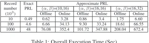
Record Exact Approximate PRL

number PRL (α, β)=(10,16) (α, β)=(16,16) (α, β)=(16,32) (103₎ _Offline _Online _Offline _Online _Offline _Online

10 0.49 0.62 3.28 0.86 3.4 1.75 6.60

[image:5.612.316.558.52.122.2]

100 4.6 6.66 34.13 9.30 33.24 18.61 66.55 1000 48 76.08 352.4 101.72 347.88 208.04 672.4

Table 1: Overall Execution Time (Sec)

protocol, for each record we creates a 2-gram set from the strings as the input to the LSH function. Our experiments were carried out on two Mac computers: party A ran on a Macbook Pro with a 2.2 GHz quad-core CPU and 16 GB RAM, party B ran on a MacPro with two 2.4 GHz six-core CPUs and 32 GB RAM.

5.1 Efficiency

In this section we evaluate the efficiency of our protocols. We first measured the overall execution time of the exact PRL proto-col. The result is shown in Table 1. We used databases with 10 thousand, 100 thousand and 1 million records in the experiment. The running time is almost linear in the size of the database. The performance is quite close to the result reported in [7].

The approximate PRL protocol splits record matching into two phases: offline and online. In the offline phase, each party inpendently processes its database to create a LSH hashtable as de-scribed in Section 4.3. Then in the online phase, the hashtable is used in oblivious Bloom intersection to generate matching pairs. In the experiment, we varied the size of databases and also param-eters(α, β)for the LSH function. Then for each combination, we measure the execution time of the offline and online phases. The re-sults are shown in Table 1 . The sizes of the databases are 10,000, 100,000 and 1,000,000. Three pairs of(α, β) used are (10,16), (16,16) and (16,32).

We can see from Table 1 that the total execution time increases almost linear in the size of the database. This is as expected be-cause the time complexity of both phases isO(n). From Table 1 we can also see that the choice of(α, β)has impact on perfor-mance. For example, when(α, β)is (10,16), (16,16) and (16,32), the total execution time is 404.08, 429.72 and 864.04 seconds re-spectively on databases with 1 million records. We can also see from the figure thatαaffects only offline execution time whileβ

affects both offline and online execution time. Whenα= 16, the offline execution time only slightly higher (about 10%) than when

α = 10. Whenβ = 32, the offline and online execution time are almost doubled comparing to whenβ= 16. This is because in-creasingαandβwill increase the cost of LSH, therefore the offline phase takes longer to finish. Increasingβalso results in a bigger hashtable with more buckets, in turn the sizes of Bloom filter and garbled Bloom filter become bigger and thus the online phase re-quires more time.

5.2 Accuracy

For the approximate PRL protocol, another very important eval-uation criterion is accuracy. The accuracy of our approximate PRL protocol is assessed by precision and recall. These metrics are based on the notions of true positive (TP), false positive (FP) and false negative (FN).

precision= _P PT P

T P+PF P

recall=P PT P

T P+PF N

A correct match is a TP, a wrong match is an FP, and a missed match is an FN.

(6)

!"#$ !"#%$ !"&$ !"&%$ '$

!$ (!!$ )!!$ *!!$ #!!$ '!!!$ !"#$%&'()'*%+(&,-'./0("-12,3!

(a) 1 Error,(α, β) = (10,16) !"#$ !"#%$ !"&$ !"&%$ !"'$ !"'%$ ($

!$ )!!$ *!!$ +!!$ &!!$ (!!!$ !"#$%&'()'*%+(&,-'./0("-12,3!

,-./01023$ 4./566$

(b) 1 Error,(α, β) = (16,16)

!"#$ !"#%$ !"&$ !"&%$ '$

!$ (!!$ )!!$ *!!$ #!!$ '!!!$ !"#$%&'()'*%+(&,-'./0("-12,3!

+,-./0/12$ 3-.455$

(c) 1 Error,(α, β) = (16,32)

!"#$ !"#%$ !"&$ !"&%$ '$

!$ (!!$ )!!$ *!!$ #!!$ '!!!$ !"#$%&'()'*%+(&,-'./0("-12,3!

(d) 2 Errors,(α, β) = (10,16) !"#$ !"#%$ !"&$ !"&%$ !"'$ !"'%$ ($

!$ )!!$ *!!$ +!!$ &!!$ (!!!$ !"#$%&'()'*%+(&,-'./0("-12,3!

,-./01023$ 4./566$

(e) 2 Errors,(α, β) = (16,16)

!"#$ !"#%$ !"&$ !"&%$ '$

!$ (!!$ )!!$ *!!$ #!!$ '!!!$ !"#$%&'()'*%+(&,-'./0("-12,3!

+,-./0/12$ 3-.455$

(f) 2 Errors,(α, β) = (16,32)

!"#$ !"#%$ !"&$ !"&%$ '$

!$ (!!$ )!!$ *!!$ #!!$ '!!!$ !"#$%&'()'*%+(&,-'./0("-12,3!

+,-./0/12$ 3-.455$

(g) 3 Errors,(α, β) = (10,16) !"#$ !"#%$ !"&$ !"&%$ !"'$ !"'%$ ($

!$ )!!$ *!!$ +!!$ &!!$ (!!!$ !"#$%&'()'*%+(&,-'./0("-12,3!

,-./01023$ 4./566$

(h) 3 Errors,(α, β) = (16,16)

!"#$ !"#%$ !"&$ !"&%$ '$

!$ (!!$ )!!$ *!!$ #!!$ '!!!$ !"#$%&'()'*%+(&,-'./0("-12,3!

+,-./0/12$ 3-.455$

[image:6.612.101.509.52.271.2]

(i) 3 Errors,(α, β) = (16,32)

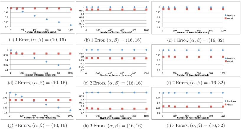
Figure 1: Accuracy with Different numbers of errors and Different(α, β)

!"#$ !"%$ !"&$ !"'$ ($

!$ (!$ )!$ *!$ +!$ ,!$ #!$

!"#$"%&'(")*+),-"#.'/)012!

(a)(α, β) = (10,16)

!"#$ !"%$ !"&$ !"'$ ($

!$ (!$ )!$ *!$ +!$ ,!$ #!$ !"#$"%&'(")*+),-"#.'/)012!

-./012134$ 5/0677$

(b)(α, β) = (16,16)

!"#$ !"%$ !"&$ !"'$ ($

!$ (!$ )!$ *!$ +!$ ,!$ #!$ !"#$"%&'(")*+),-"#.'/)012!

-./012134$ 5/0677$

[image:6.612.98.510.301.375.2]

(c)(α, β) = (16,32)

Figure 2: Accuracy with Different Overlap Percentages

several databases with different sizes, then for each database we created a modified duplicate. Each record from the original database is copied to the duplicate database with 1, 2 or 3 modifications. The modifications simulate errors such as typos, insertion, deletion, or switch of positions. We measure precision and recall with differ-ent(α, β). The results of experiments with 1 error are show in Figure 1a, 1b and 1c. We can see the protocol generally performs well with recall always higher than 0.95 and precision higher than 0.80. We can see from Figure 1a that with a smallα, we might get large amount of false positive if the database size is big. This is be-cause smallerαmeans the LSH function is more likely to produce equal hash values from distinct records. Therefore false positive in-creases. To deal with it, we can increaseα. In our experiments, set

α= 16would be enough to make false positive almost negligible. The other results in Figure 1 show that the number of errors has little effect on precision, but might affect recall. Nevertheless, if we increaseβ, then we can get a higher recall. Lower recall means more false negative. Higherβ means the LSH function is more likely to produce equal hash values from similar records. There-fore by increasingβwe can get a better recall.

In Figure 2, we show the accuracy measured with different num-ber of overlapping records and different(α, β). In the experiments, we set the size of databases to 200 thousand. In each of the ex-periment, we create the duplicate database as follows: we take a portion of the records in the original database (10%, 25% or 50%), copy them, with 1 modification, into an empty database, and then insert new records that are not in the original database until the new database contains also 200 thousand records. As we can see, when

αis small, the precision is affected by the percentage of overlap. This is because in case of less overlapped databases, more records

are irrelevant. Therefore the actual number of false positive is more significant comparing to the number of true positive, which takes down the precision. With a higher αvalue, we can get a better precision.

In summary the accuracy of our approximate protocol may be affected by multiple factors, but by setting(α, β)properly, we can ensure the accuracy is within a satisfactory bound.

5.3 Comparison

The performance of our exact PRL is better than all known pro-tocols. This is mainly due to the efficiency of the OBI protocol. As reported in [7], the OBI protocol is orders of magnitude faster than all existing private set intersection protocols. Because cur-rently the main stream exact PRL protocols are all based on private set intersection, it is not surprising that our protocol is much faster. However, it is possible that the other protocols can also use OBI, thus achieve similar performance as our protocol.

For the approximate PRL protocol, we compared our protocol performance and accuracy against two most prominent protocols, namely Vatsalan’s protocol [22] and Yakout’s protocol [24]. In the comparison, we use the results reported by the authors. The hard-ware used in their experiments is similar to or better than ours, so we believe the performance difference caused by hardware should be small thus can be ignored.

(7)

How-ever this time is measured without any encryption. Since the most costly part of the protocol is the commutative encryption, which involves public key operations, the actual execution time should be much longer with encryption. In our experience, an RSA-base commutative encryption scheme at 80-bit security normally needs more than an hour to execute 1 million encryption operations. An-other problem of Vatsalan’s protocol is that the number of the at-tributes affects performance greatly. The more atat-tributes to be used in matching, the longer it will take to do the record linking. While in our protocol, the impact of the number of attributes is negligi-ble. As for the accuracy, the precision of Vatsalan’s protocol is al-ways above 0.99. However, the recall is consistently low (less than 0.7). In our experiments, the lowest value of recall we measured is 0.759, which is still better Vatsalan’s best recall value. And as we discussed, the recall value can be improved by adjusting(α, β).

The computational complexity of Yakout’s protocol is O(n2

)

wherenis the size of the databases. The security strength of the protocol is hard to estimate because no detailed analysis was pro-vided. When the database size is 100 thousand and with the mini-mal privacy parameter (k = 4), Yakout’s protocol takes about 2.5 minutes, which is 3.5 times ((α, β)= (16,16)) or 1.75 times ((α, β)

= (16,32)) of our protocol. When the database size is 1 million, the ratios become 28.5 ((α, β)= (16,16)) or 14.1 ((α, β)= (16,32)). In their paper, the accuracy tests only used small datasets with 1000 and 5000 records. They converts string records to vectors then em-beds vectors into a metric space. The authors mentioned that if there is a large variations of records’ length, then this method is not very accurate and would result in bad matching quality. This is not a problem in our protocol.

6. CONCLUSION

In this paper, we investigated the PRL problem and proposed an exact PRL protocol and an approximate PRL protocol. The exact PRL protocol is an extension of the OBI protocol. The approxi-mate PRL protocol is built by combining LSH functions with the exact PRL protocol. We implemented the two protocols and eval-uated the protocols in terms of efficiency and accuracy. We also compared our protocols against other PRL protocols and the com-parison shows our protocols are much more efficient.

In terms of future work, we would like to validate our protocols with real world data. Another direction would be to implement and evaluate LSH functions for other similarity metrics and incorporate them into our approximate PRL protocol.

AcknowledgementZikai Wen is supported by an undergraduate

research internship from the University of Strathclyde, Changyu Dong is supported by a science faculty starter grant from the Uni-versity of Strathclyde. We thank the anonymous reviewers for their helpful comments.

7. REFERENCES

[1] R. Agrawal, A. V. Evfimievski, and R. Srikant. Information sharing across private databases. InSIGMOD Conference, pages 86–97, 2003.

[2] M. J. Atallah, F. Kerschbaum, and W. Du. Secure and private sequence comparisons. InWPES, pages 39–44, 2003. [3] A. Z. Broder, M. Charikar, A. M. Frieze, and

M. Mitzenmacher. Min-wise independent permutations (extended abstract). InSTOC, pages 327–336, 1998. [4] P. Christen and A. Pudjijono. Accurate synthetic generation

of realistic personal information. InPAKDD, pages 507–514, 2009.

[5] T. Churches and P. Christen. Some methods for blindfolded record linkage.BMC Med. Inf. & Decision Making, 4:9, 2004.

[6] E. D. Cristofaro and G. Tsudik. Practical private set intersection protocols with linear complexity. InFinancial

Cryptography, pages 143–159, 2010.

[7] C. Dong, L. Chen, and Z. Wen. When private set intersection meets big data: An efficient and scalable protocol. InACM

Conference on Computer and Communications Security,

2013.

[8] L. Dusserre, C. Quantin, and H. Bouzelat. A one way public key cryptosystem for the linkage of nominal files in epidemiological studies.Medinfo, 8 Pt 1:644–7, 1995. [9] M. J. Freedman, K. Nissim, and B. Pinkas. Efficient private

matching and set intersection. InEUROCRYPT, pages 1–19, 2004.

[10] O. Goldreich.The Foundations of Cryptography - Volume 2,

Basic Applications. Cambridge University Press, 2004.

[11] C. Hazay and Y. Lindell. Efficient protocols for set intersection and pattern matching with security against malicious and covert adversaries. InTCC, pages 155–175, 2008.

[12] Y. Huang, D. Evans, and J. Katz. Private set intersection: Are garbled circuits better than custom protocols? InNDSS, 2012.

[13] P. Indyk and R. Motwani. Approximate nearest neighbors: Towards removing the curse of dimensionality. InSTOC, pages 604–613, 1998.

[14] L. Kissner and D. X. Song. Privacy-preserving set operations. InCRYPTO, pages 241–257, 2005.

[15] M. Kuzu, M. Kantarcioglu, E. Durham, and B. Malin. A constraint satisfaction cryptanalysis of bloom filters in private record linkage. InPETS, pages 226–245, 2011. [16] C. D. Manning, P. Raghavan, and H. Schütze.Introduction to

Information Retrieval. Cambridge University Press, New

York, NY, USA, 2008.

[17] A. Rajaraman and J. D. Ullman.Mining of massive datasets. Cambridge University Press, Cambridge.

[18] P. Ravikumar and S. E. Fienberg. A secure protocol for computing string distance metrics. InIn PSDM held at ICDM, pages 40–46, 2004.

[19] M. Scannapieco, I. Figotin, E. Bertino, and A. K.

Elmagarmid. Privacy preserving schema and data matching.

InSIGMOD Conference, pages 653–664, 2007.

[20] R. Schnell, T. Bachteler, and J. Reiher. Privacy-preserving record linkage using bloom filters.BMC Medical Informatics

and Decision Making, 9(41), 2009.

[21] E. Ukkonen. Approximate string matching with q-grams and maximal matches.Theor. Comput. Sci., 92(1):191–211, 1992.

[22] D. Vatsalan, P. Christen, and V. S. Verykios. An efficient two-party protocol for approximate matching in private record linkage. InAusDM ’11, pages 125–136, Darlinghurst, Australia, Australia, 2011. Australian Computer Society, Inc. [23] D. Vatsalan, P. Christen, and V. S. Verykios. A taxonomy of

privacy-preserving record linkage techniques.Inf. Syst., 38(6):946–969, 2013.

[24] M. Yakout, M. J. Atallah, and A. K. Elmagarmid. Efficient and practical approach for private record linkage.J. Data