Methodology and Case Study on Corner Detectors
.
White Rose Research Online URL for this paper:
http://eprints.whiterose.ac.uk/792/
Article:
Rockett, Peter (2003) Performance Assessment of Feature Detection Algorithms: A
Methodology and Case Study on Corner Detectors. IEEE TRANSACTIONS ON IMAGE
PROCESSING, 12 (12). pp. 1668-1676. ISSN 1057-7149
https://doi.org/10.1109/TIP.2003.818041
[email protected] https://eprints.whiterose.ac.uk/
Reuse
Unless indicated otherwise, fulltext items are protected by copyright with all rights reserved. The copyright exception in section 29 of the Copyright, Designs and Patents Act 1988 allows the making of a single copy solely for the purpose of non-commercial research or private study within the limits of fair dealing. The publisher or other rights-holder may allow further reproduction and re-use of this version - refer to the White Rose Research Online record for this item. Where records identify the publisher as the copyright holder, users can verify any specific terms of use on the publisher’s website.
Takedown
If you consider content in White Rose Research Online to be in breach of UK law, please notify us by
1668 IEEE TRANSACTIONS ON IMAGE PROCESSING, VOL. 12, NO. 12, DECEMBER 2003
Performance Assessment of Feature
Detection Algorithms: A Methodology and
Case Study on Corner Detectors
Peter I. Rockett
Abstract—In this paper, we describe a generic methodology for
evaluating the labeling performance of feature detectors. We de-scribe a method for generating a test set and apply the method-ology to the performance assessment of three well-known corner detectors: the Kitchen-Rosenfeld, Paler et al., and Harris-Stephens corner detectors. The labeling deficiencies of each of these detec-tors is related to their discrimination ability between corners and various of the features which comprise the class of noncorners.
Index Terms—Corner detection, feature detection, performance
evaluation, ROC curves.
I. INTRODUCTION
T
HE requirement for robust and reliable corner detection is well-rehearsed in the literature [1] and in an attempt to meet this, many corner detection algorithms have been proposed over the years [2]. Unfortunately, assessment of the labeling per-formance of these detectors has been largely subjective: typi-cally detector results on real images are shown – usually with few details of the imaging conditions or detector parameters employed – and a subjective appraisal is made of the labeling performance. In recent years there has been an increasing em-phasis on quantitative performance evaluation in computer vi-sion (which we briefly review in Section II). In this paper, we present a generic methodology for assessing the performance of feature detectors. To illustrate this methodology, we describe its application to corner detectors, an area where there has been comparatively little work on performance evaluation. We return to the generic nature of the proposed methodology in Section V but in the following sections we focus on the issue of corner de-tector evaluation. We employ the well-known receiver operating characteristic (ROC) paradigm [3] to assess the performance on the two-class labeling problem (corners versus noncorners). ROCs have the advantage of mapping-out the whole range of detector operating points independent of the priors on a given labeling problem; the slope of the ROC can be related to the pos-terior probability of class membership [4] and the area under the curve (AUC) is a concise measure of performance [5] although Adams and Hand [6] have pointed-out the need for care when comparing two detectors whose ROCs cross. Central to the gen-eration of an ROC are two labeled datasets: a true feature datasetManuscript received July 17, 2002; revised March 11, 2003. The associate editor coordinating the review of this manuscript and approving it for publica-tion was Dr. Arnaud Jacquin.
The author is with the Department of Electronic and Electrical Engineering, University of Sheffield, Sheffield S1 3JD, U.K. (e-mail: p.rockett@ shef.ac.uk).
Digital Object Identifier 10.1109/TIP.2003.818041
(here, corners) and a dataset of counter-examples (noncorners) and a key challenge is to obtain two labeled sets of sufficient size to obtain statistically meaningful results. In Section II, we review relevant work on the performance evaluation of feature detectors. In the present work we employ a detailed model of the image formation process to obtain datasets of the necessary cardinality; we describe the generation of the model data in Sec-tion III.
In Section IV, we illustrate the application of the methodology presented where we examine the performance and operation of three well-known corner detectors: the Kitchen & Rosenfeld tector [7], the Paler detector [8] and the Harris & Stephens de-tector [9] also known as the Plessey corner dede-tector. One ad-vantage of the present approach is that it enables us to probe the key issues in the functioning of each of the detectors as well as assessing labeling performance in operation.
We discuss the implications and extensions of this work in Section V before offering concluding remarks in Section VI.
II. FEATUREDETECTORPERFORMANCEEVALUATION
The need for performance evaluation protocols in computer vision has greater gained acceptance in recent years—see Bowyer and Phillips [10] and Courtney et al. ([11] and refer-ences therein) for a partial survey. Most of the work done to date on evaluating the performance of feature detectors has concerned edge detection algorithms, an area initiated by the seminal work of Abdou and Pratt [12].
Heath et al. [13] have reviewed a number of methods for as-sessing edge detector performance and presented an approach of using manually labeled edges from real images to generate a dataset labeled with the ground truth from which ROC plots were produced. An ingenious aspect of the method of Heath et
al. was to introduce a “don’t know” class which was applied to
image regions where it was not possible for a human observer to unambiguously label edges. It is, however, a philosophical issue whether judging a feature detector by its concordance with the opinions of a group of human observers is legitimate—the issue would seem to hinge on the ultimate purpose of the edge detec-tion process. In addidetec-tion, whereas an edge detector would em-ploy a small image patch (maybe 3–7 pixels square) a human observer would utilize much larger-scale contextual cues.
As far as the quantitative assessment of corner detectors is concerned there has been little published work. Courtney et al. [11] describe a Monte Carlo procedure for constructing prob-ability density functions for the Harris and Stephens detector
Fig. 1. Image patch in the vicinity of a corner feature. In (a), pixel “A” should be labeled as a corner whereas in (b) pixel “B” should be labeled as a (nonobvious) noncorner.
over a very limited range of corner configurations. Mohanna and Mokhtarian [14] have employed a methodology similar to the one used by Heath et al. for edges by asking a panel of human observers to hand label corners in a set of test images; these au-thors took a feature to be a corner if more than 7 out of the 10 panel members labeled it thus and took the position of a given corner to be the average position indicated by their observers. Whatever the merits of assessing edge detectors using hand-la-beled datasets, clearly the approach is problematic in the case corners since these are fairly rare and a very large number of images would be needed to produce a statistically meaningful test set (see Section III-B). Mohanna and Mokhtarian increased the numbers of corners in their test set by affine and similarity transformation although as a consequence, not all of their test features can have been statistically independent. In addition, it is unclear whether the image location labeled by a human ob-server necessarily corresponds to the correct pixel of projection of a corner in object space.
In the following section, we describe the development of a ground truth dataset based on an accurate imaging model which overcomes the drawbacks of the approaches set-out in this sec-tion.
III. DATAMODEL
In formulating our approach, we take the objective of a corner detection process to be: To label the pixel site which
corre-sponds to the optical projection of the corner feature in object space. This introduces a subtlety in that as a corner detector of
finite (invariably odd) region of support is swept over the dig-ital image, a corner projecting in an adjacent pixel site to the location currently under consideration will produce a pattern rather similar to a corner. Nonetheless the site adjacent to the true corner should be labeled as a noncorner. This situation is illustrated in Fig. 1.
In Fig. 1(a), the pixel labeled “A” should be labeled as a corner whereas in Fig. 1(b), pixel “B”—which would present
a pattern closely resembling a corner—should nonetheless be labeled as a noncorner. In this paper we term the feature at pixel “B” a nonobvious noncorner to distinguish it from fea-tures which are obviously noncorners, such as edges and uni-form patches. Most corner detectors give a number of high re-sponses in the vicinity of a corner, a situation which is usually mitigated by nonmaximal suppression; in pattern space, corners and nonobvious noncorners thus seem to be rather close and are often confused. For this reason we explicitly consider nonob-vious noncorners.
A. Image Patch Generation
There is a sentiment in the image processing community, expressed, for example, in [13] that synthetic image data is somehow not representative of real images. We would argue that the data generated by the model used here is highly
representative of idealized features. The value of approximate
yet tractable models is beyond doubt in most fields of physics and engineering. In addition, a point that has been overlooked by most critics of synthetic data is that the design methodology of almost all detectors is the recognition of idealized features. For example, ideal step edges in the case of the Canny edge detector [15] and points of rapid, two-dimensional intensity change for the Harris-Stephens corner detector [9]. We are aware of no conventional feature detector whose development has been explicitly influenced by the need to reject clutter, texture and so on. Consequently, detector responses to the data used here are at very least, a measure of self-consistency and in practice, indicative of performance across a far wider domain. We are not aware of anybody who regards the Canny detector as of no worth because it is developed from an “unrealistic” —although eminently sensible—model of an edge.
1670 IEEE TRANSACTIONS ON IMAGE PROCESSING, VOL. 12, NO. 12, DECEMBER 2003
accurately modeling the whole optical imaging process. (We re-turn in Section V to yet further extensions.)
In the present work we assume we are imaging a “knife-edge” right-angled (“L”-) corner located on the optical axis. These “knife-edge” features are then projected onto the CCD image plane to a perfect focus through a diffraction-limited lens which in practice involves convolving the object space with an Airy function [16]. The image quality of most reasonable lenses is usually limited by diffraction through the optical aperture when stopped-down sufficiently and in this paper we have assumed an aperture of f8 as a typical figure. (Interestingly, omitting this stage – equivalent to assuming a lens of infinite diameter aper-ture – produces the most significant effect on the (mis)labeling of edges rather than corners. The influence of the optical system on the performance of feature detectors will be reported else-where.)
We then generate a set of corner patterns by applying ran-domly determined affine transformations of the optical field image projected onto the CCD. First the image is sheared to produce a corner with an random opening angle uniformly dis-tributed in the range . Then, the image is rotated by a random angle and translated by uniformly distributed displacements
If then the generated feature is a corner, otherwise it is a nonobvious noncorner. The gray levels either side of the corner were then linearly mapped to the randomly selected ranges, , . The generated data thus spans the whole pattern space of corners.
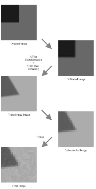
The diffracted and transformed optical signal was then integrated over the square CCD pixel sites (which, without loss of generality, we assume to exactly abut). Finally, we add Gaussian-distributed noise to the pixel values and quantize to one of 255 levels to simulate an 8-bit analog-to-digital conver-sion process in a framegrabber. Up to this final quantization stage, all calculations were performed with floating-point arithmetic. The process flow is illustrated in Fig. 2; note there is a change of scale between the first three images and the last two.
This data model thus accurately represents an idealized imaging situation and the performance of a corner detector on this dataset represents an upper bound on labeling performance which factors such as texture and clutter may well reduce; we would argue that knowing an upper bound on the performance of a detector is extremely valuable. Nonetheless, the basic methodology described here is extendable to cover factors such as finite depth-of-field (see Section V) and image clutter [17].
The particular results reported in this paper have been generated for a representative imaging setup with a lens of 25 mm focal length and an object distance of 1 meter. (In fact, the only role of the object distance is to set the optical magnification.) The CCD pixel sensors have been taken as 7.5 m on a side (15 the mean optical wavelength of 500 nm) and we have used 40 40 samples in the optical field to correspond to one CCD pixel, this figure having been determined
as sufficient to produce accurate results. The Gaussian noise had a variance of 4, being the figure observed in a number of analog camera/framegrabber combinations examined in this laboratory.
B. Size and Composition of Datasets
The labels produced on a two-class classification problem can be described by a binomial distribution with probability of suc-cess, (where is a function of the classifier operating point). We estimate over a finite sample and we would like to have confidence intervals on this measure. Confidence intervals on a binomial-distributed variate were considered by Clopper and Pearson [18] for rather small sample sizes but more generally, we can adjust the sample size to obtain a given confidence in-terval for some observed . Unfortunately, direct evaluation of the factorial quantities in the binomial distribution is problem-atic for the sample sizes of interest here but we can use an ap-proximation to the normal distribution [19] to obtain confidence intervals. In this way we conclude that for probability estimates, , 10 000 samples are sufficient to give a confidence interval of at a 95% confidence level; this range of proba-bilities is of the greatest practical interest for ROC plots.
In order to construct ROC plots we require a test set of corners and another test set of noncorners. Our corner dataset comprises 10 000 examples generated in the manner shown in Fig. 2. The set of noncorners comprises the subclasses of: nonobvious non-corners (see Fig. 1), edges and uniform patches and we can iden-tify two possible measures of performance. Firstly, we can eval-uate performance in the context of a whole image for which the composition of the noncorner set needs to reflect the proportions of the various noncorner subclasses present. Here we proceed by assuming that the prior probability of corners is and therefore the proportion of pixels which are nonobvious non-corners (NONCs) is – every corner has eight nearest neighbors which are NONCs. We further assume that around 5% of all pixel sites are edges and the remainder are uniform patches. Taking the number of NONCs as 1000, the composition of the whole image noncorner set is determined accordingly. We refer to this whole image noncorner set as dataset “A;” clearly the vast majority of this dataset is uniform patches. In a sense, evaluation on dataset “A” reflects the expectation of any pixel randomly selected from an image being labeled correctly.
In addition to studying the typical labeling performance one might expect over a given image, it is highly instructive to study the operation of a detector, in particular its ability to differen-tiate corners from the various noncorner subclasses. For this reason, we have generated a second dataset which we desig-nate “B” which comprises 10 000 of each of the noncorner sub-classes from which can obtain reliable statistics on discrimina-tion ability between, for example, corners and NONCs.
Fig. 2. Illustration of the corner generation process. Note: There is a change of scale of a factor of 40 between the first group of three images and the last two – see text for full details.
To allow other workers to assess the performance of ad-ditional corner detectors, the datasets generated here are available at http:// www.shef.ac.uk/eee/staff/pir/Datasets/Cor-nerDatasets_f8_40.zip.
IV. APPLICATION TOCORNERDETECTORS
1672 IEEE TRANSACTIONS ON IMAGE PROCESSING, VOL. 12, NO. 12, DECEMBER 2003
and Rosenfeld (KR) detector [7] is a seminal contribution to the field and forms a measure of the corner-like properties of an image point (“corner-ness”) by taking the product of gray-level curvature and the gradient magnitude. Subsequently, other au-thors have pointed-out that many other significant corner de-tectors effectively fall into this curvature-times-gradient-mag-nitude category although exact implementations may well pro-duce significant differences in performance. The KR detector here has been implemented over a 3 3 neighborhood.
We have also considered the detector of Paler et al. [8] which appears to operate on a very different principle from those detec-tors based on image calculus in that a median filtered version of the image is subtracted from the original and a cornerness mea-sure formed by multiplying the gray-level differences with the contrast over a window. Davies [20], however, has shown that subject to certain assumptions, this detector also conforms to the curvature-times-gradient-magnitude format.
The corner detector of Harris and Stephens (H-S) [9] is based on an autocorrelation measure and uses only first-derivatives to form a cornerness quantity as opposed to the second-deriva-tives used by the KR detector which are well-known to be noisy. Noble [1], however, has shown that the H-S detector again fits the curvature-times-gradient-magnitude model.
Corner detectors usually produce significant false responses in the vicinity of corners and conventionally, nonmaximal sup-pression (NMS) is used to select the peak local response. De-spite its practical utility, NMS is ultimately a “repair” stage to ameliorate detector deficiencies – in this work we focus only on the quality of the underlying corner measure on the grounds that a detector based on a good corner measure can perhaps be im-proved by NMS but a detector based on a poor measure cannot be brought up to the same quality by NMS. The minor exception to not treating NMS is with the KR detector where, arguably, an NMS stage constitutes an intrinsic part of calculating one of the possible corner measures [7].
In a number of the ROC plots which follow, the false positive fraction does not reach a value of unity even for zero threshold. (To prevent misleading discontinuities in the ROC plots we take a positive label to be the condition where ; note the strict inequality.) Where the we modify the AUC measure to be a fill-factor, AUC’, where we normalize the AUC by the maximum false positive fraction. This gives an indication of the degree to which the characteristic is filling the reachable portion of the plot; an AUC’ measure of unity is ideal.
A. Kitchen and Rosenfeld Detector [7]
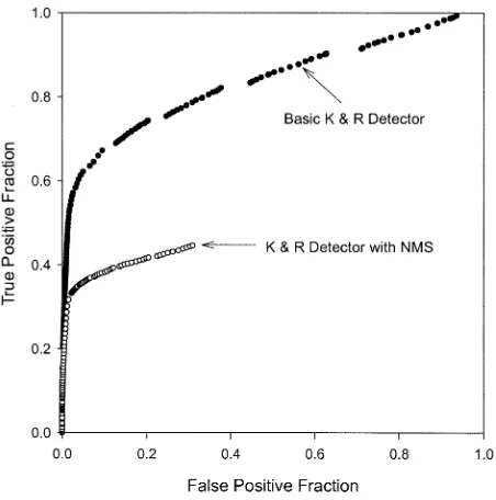
The ROC plot for the basic KR detector generated with dataset “A” (reflecting whole image labeling) but without nonmaximally suppressing gradient values is shown in the upper curve of Fig. 3. (The gaps in the plot are caused by calculating the cornerness measure over quantized gray-level values rather than insufficient data.)
[image:6.612.316.542.61.289.2]Clearly the basic KR detector is rather poor and we can in-vestigate the reasons for this from the response to each sub-class (dataset “B”) plotted against threshold in Fig. 4 where the thresholds span the range of practically useful values.
Fig. 3. ROC plots for the basic and nonmaximally suppressed KR detector.
Fig. 4. Labeling response of the basic Kitchen and Rosenfeld detector.
[image:6.612.308.552.331.516.2]Fig. 5. Labeling response of the Kitchen and Rosenfeld detector with nonmaximal suppression.
results consistent with previous subjective evaluation as well as providing a means to quantify the effect.
B. Paler, Föglein, Illingworth, Kittler Detector [8]
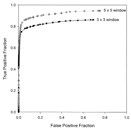
The Paler detector is based on the observation that median filtering does not greatly distort edges but does affect corners. Here the size of the median filter window is a parameter. The ROC plots (dataset A) for both 3 3 and 5 5 windows are shown in Fig. 6; using a 7 7 window does not produce a sig-nificantly better ROC plot than the 5 5 detector. The conclu-sion from Fig. 6 is in agreement with Davies [20] that a 5 5 window gives somewhat better results.
The labeling responses (over dataset B) for both the 3 3 and 5 5 windows are shown in Figs. 7 and 8, respectively. It is noteworthy that although the 5 5 detector has an improved selectivity for corners, the response for all of the noncorner classes, particularly NONCs, is also increased. This would tend to suggest that the 5 5 detector would suffer from an increased rate of false responses in the vicinity of a corner but if these could be filtered by nonmaximal suppression then the larger window size may be preferable. Although not shown here, the trend of increasing window size reducing the corner/NONC dis-crimination is further worsened for the 7 7 detector.
C. Harris & Stephens Detector [9]
The Harris and Stephens detector proceeds by forming a set of partial first derivatives, whence
(1)
where is a zero-mean Gaussian smoothing kernel of variance, and is the convolution operator. Forming the symmetric matrix:
[image:7.612.42.289.61.247.2](2)
Fig. 6. ROC plots for the Paler detector for 32 3 and 5 2 5 windows.
Fig. 7. Labeling response for 32 3 Paler detector.
[image:7.612.306.552.315.500.2] [image:7.612.293.551.549.734.2]1674 IEEE TRANSACTIONS ON IMAGE PROCESSING, VOL. 12, NO. 12, DECEMBER 2003
[image:8.612.303.552.63.243.2]Fig. 9. ROC plots for the Harris-Stephens detector. Filled circles are fork = 0:04 and open triangles for k = 0 – see text for explanation.
Fig. 10. Labeling response for Harris-Stephens detector fork = 0:04.
leads to the “inspired formulation” [9] of the cornerness mea-sure
(3) It is interesting to note that Gaussian convolutions in (1) were justified by Harris and Stephens as needed to suppress noise in the partial derivatives, but it is clear from the above (1)–(3) that either omitting this stage or smoothing before
calcu-lating , , results in a cornerness measure which is iden-tically zero. Thus, rather than merely suppressing noise, the Gaussian convolution would appear to be fundamental to the operation of the detector in that it isotropically modifies the fre-quency spectra of the various quantities – in this sense it func-tions similarly to the median-filtering stage in the Paler detector. This pivotal role of the Gaussian filter does not hitherto seem to have been explicitly noted in the literature.
The ROC plot for the H-S detector for ; is shown in Fig. 9 along with the plot for the case where . It is clear that the detector with is superior and achieves a
Fig. 11. Labeling response for Harris-Stephens detector fork = 0. Note the greatly increased response to edges over Fig. 10.
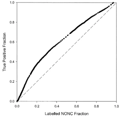
Fig. 12. ROC plot for Harris-Stephens detector for = 1 and k = 0:04. Here the noncorner class comprises only nonobvious noncorners (NONCs). The dashed line is the ROC characteristic for random guessing.
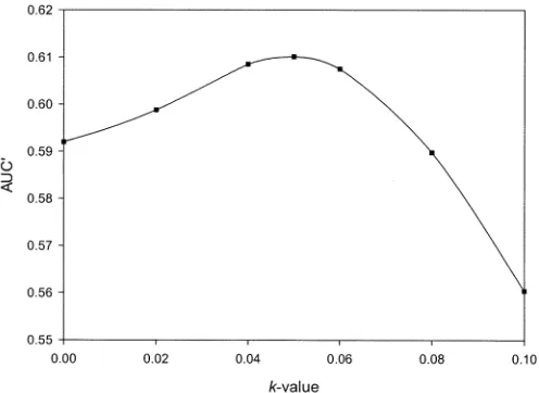
[image:8.612.323.530.286.489.2] [image:8.612.43.289.306.488.2]Fig. 13. AUC’ measure versusk-value for the Harris-Stephens detector. Note the suppressed zero on the ordinate.
As a final example of the evaluation methodology presented here, we examine the optimal setting of one of the parameters in the H-S detector. Harris and Stephens [9] mentioned no value for in (3) but 0.04 appears to be widely used. We have applied the present methodology to determining the -value which opti-mizes the AUC’ measure for the family of corner versus NONC ROC plots such as Fig. 12. A plot of AUC’ versus -value (for ) is shown if Fig. 13 which suggests that a value of 0.05 is optimal, at least for the present imaging conditions. The im-provement in performance is, however, very small and thus the figure of seems well-founded. Nonetheless, Fig. 13 illustrates an important application of the present approach to optimization of detector parameters with respect quantitative la-beling performance.
V. DISCUSSION ANDFUTUREWORK
Clearly the present methodology generates idealized image examples which can be viewed as yielding an upper bound on performance; if a feature detector cannot perform well on such “clean” examples then it unlikely to perform well on real-world examples contaminated by clutter and texture. Although the il-lustrations used here relate to corner detection, the methodology is generic in the sense that it can be used to produce test data for any arbitrary feature. All that is required is a high-resolution image of the idealized feature to replace the first image in Fig. 2. The construction of a suitable dataset proceeds analogously.
In the present paper, in using the Airy function for the point spread function we have implicitly assumed quasimonochro-matic incoherent illumination. Extension to broadband illumi-nation for a source of arbitrary spectrum is straightforward; fur-ther extension to fully or partially coherent illumination is also possible [16] although somewhat more involved. Here, for sim-plicity we have also assumed that the image features are in per-fect focus but a finite depth of optical field can be modeled via the Lommel functions [16]. More generally, the influence of imaging conditions on the performance of feature detectors is an area that has not received much attention [22] – this too is an avenue of future research.
Most of the previous analyses of corner detectors have as-sumed a real-valued, continuous intensity function, for example [1], [2], [20]. Clearly images are discrete and quantized and therefore it is conceivable that even different implementations of the same algorithm may produce different results. Despite each of the three corner detectors considered having been shown to broadly conform to the curvature-times-gradient-magnitude form, it is interesting that each has its own particular short-coming. A detailed comparison of corner detectors will be the subject of future publication.
In this paper we have approached the issue of localization
implicitly by taking a true positive to be a label in the pixel in
which the object-space corner projects – if a neighboring pixel is labeled this is counted as a false positive. Clearly localization and its interaction with nonmaximal suppression is complex and again, will be the subject of further research.
The present use of a standardized methodology allows a quantitative comparison or the objective evaluation of novel detectors – we see this as the key contribution of the present paper. Nonetheless, it is reassuring that the present results agree broadly with previous subjective observations.
VI. CONCLUSIONS
In this paper, we have described a methodology for the per-formance evaluation of feature detectors. The evaluation frame-work is generic but to illustrate the procedure, we have analyzed three well-known corner detectors. In particular, we have been able to pinpoint the deficiencies of each detector which we have related to its ability to discriminate between corners and various of the noncorner classes.
REFERENCES
[1] J. A. Noble, “Finding corners,” Image Vis. Comput., vol. 6, no. 2, pp. 121–128, May 1988.
[2] K. Rohr, “Localization properties of direct corner detectors,” Int. J.
Math. Imag. Vis., vol. 4, no. 2, pp. 139–150, 1994.
[3] M. H. Zweig and G. Campbell, “Receiver-operating characteristic (ROC) plots: A fundamental evaluation tool in clinical medicine,” Clin.
Chem., vol. 39, no. 4, pp. 561–577, 1993.
[4] T. Kanungo and R. M. Haralick, “Receiver operating characteristic curves and optimal bayesian operating points,” Proc. IEEE Int. Conf.
Image Processing, pp. 256–259, Oct. 1995.
[5] A. P. Bradley, “The use of the area under the ROC curve in the evaluation of machine learning algorithms,” Pattern Recognit., vol. 30, no. 7, pp. 1145–1159, 1997.
[6] N. M. Adams and D. J. Hand, “Comparing classifiers when misal-location costs are uncertain,” Pattern Recognit., vol. 32, no. 7, pp. 1139–1147, July 1999.
[7] L. Kitchen and A. Rosenfeld, “Gray-level corner detection,” Pattern
Recognit. Lett., vol. 1, no. 2, pp. 95–102, Dec. 1982.
[8] K. Paler, J. Föglein, J. Illingworth, and J. Kittler, “Local ordered grey-levels as an aid to corner detection,” Pattern Recognit., vol. 17, no. 5, pp. 535–543, 1984.
[9] C. Harris and M. Stephens, “A combined corner and edge detector,” in
Proc. 4th Alvey Vision Conf., Manchester, U.K., 1988, pp. 147–151.
[10] K. W. Bowyer and P. J. Phillips, “Overview of work in empirical eval-uation of computer vision algorithms,” in Empirical Evaleval-uation
Tech-niques in Computer Vision, K. W. Bowyer and P. J. Phillips, Eds. New York: IEEE Computer Soc. Press, 1998.
[11] P. Courtney, N. A. Thacker, and A. F. Clark, “Algorithmic modeling for performance evaluation,” Mach. Vis. Applicat., vol. 9, no. 5-6, pp. 219–228, 1997.
1676 IEEE TRANSACTIONS ON IMAGE PROCESSING, VOL. 12, NO. 12, DECEMBER 2003
[13] M. D. Heath, S. Sarkar, T. Sanocki, and K. W. Bowyer, “A robust visual method for assessing the relative performance of edge-detection algo-rithms,” IEEE Trans. Pattern Analysis and Machine Intelligence, vol. 19, no. 12, pp. 1338–1359, Dec 1997.
[14] F. Mohanna and F. Mokhtarian, “Performance evaluation of corner detection algorithms under similarity and affine transforms,” in Proc.
British Machine Vision Conf. (BMVC2001), Manchester, U.K., Sept.
2001, pp. 353–362.
[15] J. Canny, “A computational approach to edge detection,” IEEE Trans.
Pattern Anal. Machine Intell., vol. 8, pp. 679–698, Nov. 1986.
[16] M. Born and E. Wolf, Principles of Optics, 7th ed. Cambridge, U.K.: Cambridge Univ. Press, 1999.
[17] T. Kanungo, M. Y. Jaisihma, J. Palmer, and R. M. Haralick, “A method-ology for quantitative performance evaluation of edge detection algo-rithms,” IEEE Trans. Image Processing, vol. 4, pp. 1667–1674, Dec. 1995.
[18] C. J. Clopper and E. S. Pearson, “The use of confidence or fiducial limits illustrated in the case of the binomial,” Biometrika, vol. 26, no. 3-4, pp. 404–413, 1934.
[19] D. A. Berry and B. W. Lindgren, Statistics: Theory and Methods, 2nd ed. Belmont, CA: Wadsworth, 1996, pp. 135–136.
[20] E. R. Davies, “Median-based methods of corner detection,” in Proc. 4th
Int. Conf. Pattern Recognit., Cambridge, U.K., Mar. 1988, pp. 360–369.
[21] Z. Zheng, H. Wang, and E. K. Teoh, “Analysis of gray level corner de-tection,” Pattern Recognit. Lett., vol. 20, no. 2, pp. 149–162, Feb. 1999. [22] R. G. White and R. A. Schowengerdt, “Effect of point-spread functions on precision edge measurements,” J. Opt. Soc. Amer., vol. 11, no. 10, pp. 2593–2603, Oct. 1994.
Peter I. Rockett was born in London, U.K., in
1954. He received the B.Sc. degree in electronic engineering in 1976, the M.Sc. degree in solid-state electronics in 1977, and the Ph.D. degree in semi-conductor physics in 1980.