This is a repository copy of
Speaker verification using sequence discriminant support
vector machines
.
White Rose Research Online URL for this paper:
http://eprints.whiterose.ac.uk/813/
Article:
Wan, V. and Renals, S. (2005) Speaker verification using sequence discriminant support
vector machines. IEEE Transactions on Speech and Audio Processing, 13 (2). pp.
203-210. ISSN 1063-6676
https://doi.org/10.1109/TSA.2004.841042
[email protected] https://eprints.whiterose.ac.uk/
Reuse
Unless indicated otherwise, fulltext items are protected by copyright with all rights reserved. The copyright exception in section 29 of the Copyright, Designs and Patents Act 1988 allows the making of a single copy solely for the purpose of non-commercial research or private study within the limits of fair dealing. The publisher or other rights-holder may allow further reproduction and re-use of this version - refer to the White Rose Research Online record for this item. Where records identify the publisher as the copyright holder, users can verify any specific terms of use on the publisher’s website.
Takedown
If you consider content in White Rose Research Online to be in breach of UK law, please notify us by
Speaker Verification Using Sequence Discriminant
Support Vector Machines
Vincent Wan and Steve Renals
, Member, IEEE
Abstract—This paper presents a text-independent speaker veri-fication system using support vector machines (SVMs) with score-space kernels. Score-score-space kernels generalize Fisher kernels and are based on underlying generative models such as Gaussian mix-ture models (GMMs). This approach provides direct discrimina-tion between whole sequences, in contrast with the frame-level ap-proaches at the heart of most current systems. The resultant SVMs have a very high dimensionality since it is related to the number of parameters in the underlying generative model. To address prob-lems that arise in the resultant optimization we introduce a tech-nique called spherical normalization that preconditions the Hes-sian matrix. We have performed speaker verification experiments using the PolyVar database. The SVM system presented here re-duces the relative error rates by 34% compared to a GMM likeli-hood ratio system.
Index Terms—Fisher kernel, score-space kernel, speaker verifi-cation, support vector machine.
I. INTRODUCTION
C
URRENT state-of-the-art speaker verification systems are based on generative speaker models, typically Gaussian mixture models (GMMs) and hidden Markov models (HMMs) [1]. These models usually operate at the frame-level with an overall sequence score obtained by averaging the likelihoods of each frame in the sequence or via the use of an HMM. More accurate verification systems may be constructed by placing these generative models in a discriminative framework, for ex-ample taking the likelihood ratio between the model for a par-ticular speaker and a more general world model [2]. A limi-tation of these approaches arises from the fact that discrimi-nation occurs between frames, whereas speaker verification is concerned with sequence discrimination. Since a discriminative classifier discards information that its objective function con-siders irrelevant, frame discrimination approaches may inadver-tently discard relevant information. In this paper we describe an approach to speaker verification based on the support vector ma-chine (SVM) [3], [4] that enables direct discrimination between sequences.An SVM has many desirable properties including the ability to classify sparse data without over-training and to make
non-Manuscript received July 11, 2003; revised October 13, 2003. The work of V. Wan was supported by a Motorola studentship. The associate editor coordinating the review of this manuscript and approving it for publication was Dr. Geoffrey Zweig.
V. Wan is with the Department of Computer Science, University of Sheffield, Sheffield S1 4DP, U.K. (e-mail: [email protected]).
S. Renals was with the Department of Computer Science, University of Sheffield, Sheffield S1 4DP, U.K. He is now with the Centre for Speech Technology Research, University of Edinburgh, Edinburgh EH8 9LW, U.K. (e-mail: [email protected]).
Digital Object Identifier 10.1109/TSA.2004.841042
linear decisions via kernel functions. However, due to certain practical limitations the SVM has not gained widespread usage in mainstream applications. Initial speaker recognition work using SVMs by Schmidt and Gish [5] highlighted the main problem: SVMs become inefficient when the the number of training frames is large. This can be overcome by using special kernels to classify sequences instead of frames. The family of score-space kernels [6] are such kernels that enable sequence discrimination. Score-space kernels include the Fisher kernel [7] and map a complete sequence onto a single point in a high-dimensional space by exploiting generative models. The Fisher kernel has been applied to speaker recognition with limited success [8], [9].
We have applied the score-space kernel SVM approach to text-independent speaker verification, extending some previous work that employed frame-discriminant SVMs [10], [11]. We performed experiments on the PolyVar database [12] and report error rates that are better than a GMM likelihood ratio system by 34% and better than the current state-of-the-art system by 25%. The structure of this paper is as follows: Section II provides an overview of GMM speaker verification systems; Section III reviews SVMs for classification; sequence kernels and methods for normalizing them are described in Section IV; experimental evaluation and results are presented in Section V; Section VI concludes the paper.
II. GMM-BASEDSPEAKERVERIFICATION
An component Gaussian mixture for dimensional input vectors has the following form:
(1)
where is the likelihood of input vector given the mixture model, . The mixture model consists of a weighted sum over Gaussian densities, each parameterized by a mean vector and a covariance matrix . The coefficients, , are the mixture weights, which are constrained to be nonnegative and must sum to one. The parameters of a Gaussian mixture model, , , and for may be estimated using the maximum likelihood criterion and the EM (expecta-tion-maximization) algorithm [13], [14].
For reasons of both modeling and estimation, it is usual to em-ploy GMMs consisting of components with diagonal covariance matrices. A detailed discussion on the application of GMMs to speaker modeling can be found in [15]. The basic method
204 IEEE TRANSACTIONS ON SPEECH AND AUDIO PROCESSING, VOL. 13, NO. 2, MARCH 2005
is straightforward. A GMM (theclient model) is trained using maximum likelihood to estimate the probability density func-tion of the client speaker. The probability
that an utterance is generated by the model is used as the utterance score, estimated by the mean log like-lihood over the following sequence:
(2)
The utterance score is used to make a decision by comparing it against a threshold that has been chosen for a desired tradeoff between detection error types.
GMM likelihood ratio (GMM-LR) speaker verification may be posed as a discriminative problem, with the objective of assigning high scores to those frames, , that are specific to the client and low scores to frames that are common to most speakers. To achieve this a second GMM (the world model) may be used to model the properties of speech signals common to all speakers, with parameters estimated from a large number of background speakers. A discriminative score may then be obtained by taking the log-likelihood ratio of the client model to the world model, , which is equivalent to the difference between their log-likelihood scores. Again, the mean of the frame scores is taken across the sequence
(3)
(4)
(5)
We call this approach the GMM-LR, and in practice it produces more accurate speaker verification systems. Reynolds [2] used the GMM-LR approach for speaker verification. The GMM-LR method is a simple yet powerful approach and is used here as a baseline.
By Bayes’ decision rule, (5) is optimal so long as the client and impostors are well modeled. Bengio and Mariéthoz [16] proposed that the probability estimates are not perfect and that a more accurate version would be
(6)
where , , and are adjustable parameters estimated using a support vector machine (SVM) for which the input is the two-dimensional (2-D) vector composed of the client and world models’ log likelihoods. This results in a small improvement in accuracy as discussed in Section V.
III. SUPPORTVECTORCLASSIFICATION
In its basic form, the SVM is a binary linear classifier. It is described in detail by Vapnik [3] and in Burges’ tutorial [4]. Given a set of linearly separable two-class training data, there are many possible solutions for a discriminative classifier. In the case of the SVM, a separating hyperplane is chosen so as to maximize themarginbetween the two classes. Essentially, this
involves orienting the separating hyperplane to be perpendicular to the shortest line separating the convex hulls of the training data for each class, and locating it midway along this line.
Let the separating hyperplane be defined by , where is its normal. For linearly separable data labeled
, , , , the optimum
boundary chosen according to the maximum margin criterion is found by minimizing the objective function
subject to for all (7)
The solution for the optimum boundary is a linear combi-nation of a subset of the training data, , : the support vectors. These support vectors define the margin edges and satisfy the equality . Data may be clas-sified by computing the sign of .
Generally, the data are not separable and the above inequali-ties cannot be satisfied. In this case, we may introduce “slack” variables which represent the amount by which each point is misclassified. In this case, the objective function is reformulated as
subject to for all (8)
The second term on the right-hand side of (8) is theempirical risk associated with those points that are misclassified or lie within the margin. is a cost function and is a hyper-param-eter that trades off the effects of minimizing the empirical risk against maximizing the margin. The first term can be thought of as a regularization term, derived from maximizing the margin, which gives the SVM its ability to generalize well on sparse training data. This property will be seen to be important when classifying sequences.
The linear-error cost function is most commonly used since it is robust to outliers. The dual formulation (which is more con-veniently solved) of (8) with is
(9)
subject to (10)
in which is the set of Lagrange multipliers of the constraints in the primal optimization problem [4]. The dual can be solved using standard quadratic programming tech-niques. The optimum decision boundary is given by
(11)
functions. The hyperplane is constructed in the feature space and intersects with the manifold creating a nonlinear boundary in the input space. In practice, the mapping is achieved by re-placing the value of dot products between two vectors in input space with the value that results when the same dot product is carried out in the feature space. The dot product in the feature space is expressed conveniently by the kernel as some function of the two vectors in input space. The polynomial and radial basis function (RBF) kernels are commonly used, and take the form
(12)
and
(13)
respectively, where is the order of the polynomial and is the width of the radial basis function. The dual for the nonlinear case is thus
(14)
subject to (15)
The use of kernels means that an explicit transformation of the data to the feature space is not required.
IV. DISCRIMINATIVESEQUENCECLASSIFICATION
The approaches to speaker verification outlined in Section II are discriminative between frames rather than between com-plete utterances. Discriminative classification of sequences is difficult since sequences have different lengths. However, if a mapping from a variable-length sequence to a fixed-length vector can be achieved, then standard classification proce-dures may be applied. Such a mapping was first developed by Jaakkola and Haussler [7] and is known as theFisher kernel. This approach was generalized by Smith and Gales [18], [19] as a technique referred to asscore-spaces. Using these approaches for whole sequence classification results in a sparse data problem, for which SVMs are well suited: a set of sequences are mapped to a comparatively high-dimensional feature space. Furthermore, the concept of mapping each sequence to a fea-ture space may be interpreted as an SVM kernel. We shall now describe the score-space transformations that we have used.
A. Score-Spaces
Score-space kernels [6], [18], [19], which generalize Fisher kernels [7], enable SVMs to classify whole sequences by ex-ploiting a set of parametric generative models. In this approach, a variable-length sequence is mapped explicitly onto a single point in a fixed-dimension space, thescore-space. Such a map-ping is achieved by applying some operator to the likelihood score of a generative model. Hence, the fixed-dimension
score-TABLE I
SOMEEXAMPLES OFSCOREOPERATORS
space allows a dot product to be computed between two se-quences even if they were originally different lengths. This sec-tion first describes a generic formulasec-tion to achieve such map-pings followed by a detailed explaination of some special cases of the score-space method: the Fisher kernel [7] and the likeli-hood ratio kernel.
The score-space is defined by and derived from the likeli-hood score of a set of generative models, . The generic formulation for mapping a sequence
to the score-space is given by
(16)
where is called thescore-vector, , a function of the scores of the set of generative models, is called thescore-argumentand is thescore-operatorthat maps the scalar score-argument to the score-space. The properties of the resulting score-space depend upon the choice of operator and argument that is used. Several options for score-operators were proposed by Smithet al.[6] and are summarized in Table I.
Almost any function may be used as a score-argument. We shall show two specific cases that lead to the likelihood score-space kernel (more commonly known as the Fisher kernel [7]) and the likelihood ratio score-space kernel.
1) The Likelihood Score-Space: The likelihood score-space is obtained by setting the score-argument to be the log likelihood of a generative model parameterized by , and choosing the first derivative score-operator from Table I
(17) (18)
This mapping, known as theFishermapping, was first devel-oped and applied to biological sequence analysis by Jaakkola and Haussler [7].
Each component of the score-space corresponds to the derivative of the log-likelihood score with respect to one of the parameters of the model. In some ways, it is a measure of how well the sequence matches the model. Consider a generative model trained using the maximum likelihood criterion and gra-dient descent. In order to maximize the likelihood of a given sequence, the same set of derivatives to (18) must be computed so that the parameters may be updated. When the derivatives are small, then the likelihood may be close to a local maximum; when the derivatives are large, then the likelihood has yet to reach a maximum. Whether the derivatives will provide addi-tional information that is not already encoded in the likelihood score may be examined by augmenting the score-vector with the score-argument (the log-likelihood score in this case)
206 IEEE TRANSACTIONS ON SPEECH AND AUDIO PROCESSING, VOL. 13, NO. 2, MARCH 2005
2) Likelihood Ratio Score-Space: An alternative score-ar-gument is the ratio of two generative models, and
(20)
where . The corresponding mapping using the first derivative score-operator is
(21)
and again the score-argument may be added to the score-space
(22)
The likelihood ratio score-space is motivated by the GMM-LR classifier described in Section II. In the same way that the GMM-LR is a more discriminative classifier than a single GMM, so should the likelihood ratio score-space kernel be. A GMM likelihood ratio forces the classifier to model the class boundaries more accurately. The discrimination information encoded in the likelihood ratio score will also be in its deriva-tives.
B. Computing the Score-Vectors
In this section, we derive the formulae for computing deriva-tives of the log likelihoods when the generative model is a diag-onal covariance GMM. The formulae for the derivatives when the generative model is an HMM may be found in [6].
Let
(23)
so that the diagonal covariance GMM likelihood is
(24)
where is the set of parameters in the GMM, . In particular, is the prior of the th Gaussian component of the GMM, is the mean vector of the th component, and is the corresponding diagonal covariance vector. The superscript on the mean and covariance enumerate the components of the vectors. is the number of Gaussians that make up the mixture model and is the dimensionality of the input vectors with
components .
The global log likelihood of a sequence is
(25)
where is the number of frames in the sequence. From (18), the score-vector is the vector of the derivatives with respect to each parameter of the log of (25). The derivatives are with re-spect to the covariances, means and priors of the Gaussian mix-ture model. The derivative with respect to the th prior is
(26)
The derivative with respect to the th component of the th mean is
(27)
The derivative with respect to the th component of the th co-variance is
(28)
The likelihood score-vector can then be expressed as
(29)
for and .
The likelihood ratio kernel is also computed using (26)–(29). The score-vectors of the likelihood ratio kernel (21) can be ex-pressed as the difference of two terms
(30) Let be the vector of all parameters that exist in both models, and . The derivatives of
with respect to the parameters in are zero and vice-versa. Thus, can be split so that the derivatives are computed with respect to one model at a time. When the differentiated parameter belongs to model , then
(31)
is computed. Likewise, when the parameter belongs to model , then
is computed. These derivatives are identical to the derivatives computed by the Fisher kernel. The likelihood ratio score-vector is
(33)
From (29) and (33), it can be seen that the dimensionality of the score-space is equal to the total number of parameters in the generative models. Having mapped the sequence to the score-space, any discriminative classifier may be used to classify vec-tors and hence obtain a classification for the complete sequence. However, it is not unusual for generative models to have several thousand parameters. This means that the discriminative classi-fier must be able to classify vectors of that size. Classiclassi-fiers such as multilayer perceptrons cannot be easily trained on such data due to problems in parameterization. The SVM, fortunately, is well suited to classify high-dimensional data.
C. Score-Space Normalization
SVMs are not invariant to linear transformations in feature space, so normalization of the feature vectors is desirable. We used two stages of normalization: whitening the data in the score-space by normalizing the components of the vectors, , to zero mean and unit variance; then applying spher-ical normalization, which may be interpreted as a Hessian preconditioning step and involves making a further nonlinear transformation to a higher dimension space.
1) Score-Space Whitening: For a given score-space, the metric of the space is determined by the generative model(s) and is generally non-Euclidean. The dot product in a non-Eu-clidean space is defined as where is a matrix that maps the vectors to a Euclidean space. A kernel constructed from any of the above mappings is
(34)
where is the metric of the space and the subscript on enumerates the sequences. In Euclidean space, is the identity matrix. In the case of the log-likelihood score-space mapping, is the inverse Fisher information matrix (the inverse of the covariance matrix of the score-vectors)
(35)
where and is the expectation
operator.
This can be interpreted as a whitening step where the score-vector components are normalized to zero mean and unit variance (i.e., the basis vectors of the score-space are mapped to an orthonormal set). Whitening is important since SVMs are not invariant to linear transformations in the feature space. Consider a 2-D space where the variance in one dimension is significantly higher than in the other. A dot product in this case will be dominated by the high variance component, effectively reducing the dimensionality of the space to one.
[image:6.594.377.474.66.165.2]Computing dot products in score-space relies on the ability to estimate a full covariance matrix, which will normalize the scaling in each dimension and make the principal component
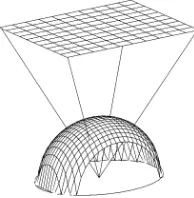
Fig. 1. Spherical vector-length normalization: mapping onto a sphere.
axes orthogonal. However, the score-space space dimension-ality, which is equal to the number of parameters in the gen-erative model, may be large thus making estimation imprac-tical. The required computation may be reduced by normalizing with a diagonal covariance matrix (so the scale of each dimen-sion will be the same), or a block diagonal covariance matrix (making some of the principal component axes orthogonal).
2) Spherical Normalization: Spherical normalization, de-veloped in the context of SVMs using high order polynomial kernels [11], is a preconditioning step employing a transfor-mation that maps each feature vector onto the surface of a unit hypersphere embedded in a space that has one dimension more than the feature vector itself.
Dot products between high-dimensional vectors may lead to an ill-conditioned Hessian since the dynamic range of the result is large. This occurs even when each individual component of the vectors has been normalized to zero mean and unit variance. In particular, score-space kernels based on generative models that have many tens of thousands (or more) of parameters are likely to suffer from ill-conditioning. It is possible to compress the dynamic range of a dot product by exploiting its cosine in-terpretation, i.e., . If the vectors have unit length, then the dot product is just the cosine of the angle in be-tween and the result must be in the range to .
A vector can be normalized easily by dividing by its Eu-clidean length. But this results in information loss causing greater classification uncertainty. For example, two points in the input space represented by and will both be normalized to . Alternatively, normalization without information loss may be done by projecting to a higher dimensional space. Consider the mapping from a 2-D plane to a 3-D unit sphere, as in Fig. 1. Any point in 2-D space may be mapped onto the surface of a unit sphere in 3-D space. The new vectors representing the data are the unit vectors from the center of the sphere to its surface. The mapping is reversible so no information is lost. We call this spherical vector-length normalization, or spherical normalization for short.
208 IEEE TRANSACTIONS ON SPEECH AND AUDIO PROCESSING, VOL. 13, NO. 2, MARCH 2005
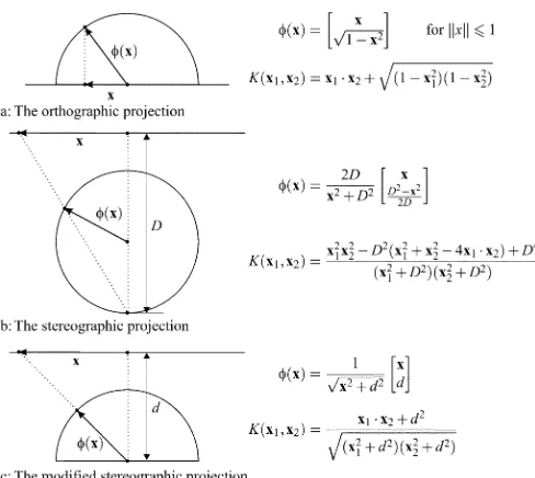
Fig. 2. Spherical vector-length normalization: various ways of projecting data onto unit hyperspheres.
The orthographic projection [Fig. 2(a)] is limited since the input data are restricted to lie within a small finite region directly beneath the hemisphere. The stereographic projection [Fig. 2(b)] does not suffer from this restriction but the space represented by the sphere wraps around. With this projection, points located at and in the input space project to the same point on the hypersphere. We used the modified stereographic projection [Fig. 2(c)] because it does not suffer from these issues. The projection is made by augmenting a vector with a constant and normalizing the new vector by its Euclidean length.
For the score-space kernels presented here, the mapping ap-plied explicitly to the score-vectors is
(36) where is the whitened score-vector of the sequence . The spherically normalized sequence kernel be-comes
(37)
Spherical normalization is discussed in greater depth, and in the context of polynomial and RBF kernels, in [20].
V. EXPERIMENTS
We carried out a number of development experiments [10] using the YOHO database [21]. Following these, we evaluated these approaches using text-independent speaker verification on the PolyVar database [12]. The PolyVar database consists of 38 client speakers, 24 male and 14 female, recorded over a tele-phone network. 85 utterances were recorded from each speaker in 5 sessions, with 17 utterances per session. There are also 952 impostor utterances from 56 speakers, each contributing 17 ut-terances in a single session. The evaluation followed the pro-tocol for speaker model training and testing used on the
Euro-pean Telematics PICASSO project [22]. Approximately 1000 test utterances, including both client and impostors, were pre-sented for each client speaker.
The speech was parameterized as 12th-order perceptual linear prediction (PLP) cepstral coefficients, computed using a 32-ms window and a 10-ms frame shift. The 12 cepstral coefficients were augmented with an energy term and first and second derivatives were estimated, resulting in frames of 39 dimensions. Cepstral mean subtraction was applied to remove the effects of the communication channel. Silence frames within each utterance were segmented out using a multilayer perceptron pre-trained on a different dataset [23].
Our baseline systems for these experiments were based on GMMs. The simplest baseline uses the client model only (2). State-of-the-art results for this database have been obtained by a GMM-LR system (5) and a modified GMM-LR/SVM system (6) in which the likelihood ratio is parameterized using an SVM to estimate the parameters [16]. To enable a direct comparison, the GMMs used in the experiments here were trained using iden-tical conditions to those used in [16] in which cross-validation was used to estimate the optimal model complexity. This re-sulted in a world GMM containing 1000 Gaussian components, and client GMMs containing 200 Gaussian components.
Using the GMM-LR system on PolyVar, a text independent speaker verification result of 5.55% minimum half total error rate (HTER)1 was reported on the PolyVar test data using 19 speakers.2 A 4.73% minimum HTER was reported for the GMM-LR/SVM [16]. We replicated these results: the results for 38 speakers are shown in Table II, and the corresponding DET curves are shown in Fig. 3.
We applied the score-space kernel approaches to PolyVar, based on the GMMs that made up the baseline systems. These GMMs were used to generate the score-spaces used by the ker-nels discussed in Section IV. Using one of these kerker-nels, each complete utterance was mapped onto a single score-vector. An SVM was trained for each client speaker using a total of 1 037 utterances (85 client and 952 background utterances), each mapped to the score-space. The SVM optimization problem for training sets of this size is straightforward and does not require any of the special techniques that have been developed to train SVMs on large quantities of data. We trained SVMs using the following kernels:
• Fisher kernel (18);
• Fisher kernel with argument (19); • LR kernel (21);
• LR kernel with argument (22).
The Fisher kernel uses the derivatives of the client GMMs from the baseline systems to achieve the mapping to score-space, whereas the LR kernel uses both the client and world models. The number of parameters in the GMM and GMM-LR baselines are 15 800 and 94 800, respectively. The score-space dimensionalities of the Fisher and LR kernels are thus 15 800
1The HTER is the arithmetic mean of the false acceptance rate and the false
rejection rate at a given threshold. The threshold can be adjusted to minimize the HTER.
2Bengio and Mariéthoz [16] used 19 speakers for development and the
TABLE II
RESULTS OF THEPOLYVAREXPERIMENTS. THEGMM BASELINE HAS200 DIAGONALCOVARIANCEGAUSSIANCOMPONENTS FORMODELLINGCLIENTS.
THEGMM-LR CONSISTS OF THEABOVEPLUS AWORLDGMM WITH1000 DIAGONALCOVARIANCEGAUSSIANS. THEGMM-LR/SVM USES THESAME
CLIENT ANDWORLDGMMS BUTCOMPUTES AWEIGHTEDLOGLIKELIHOOD
[image:8.594.47.278.147.529.2]RATIO. THEFISHERKERNELEXPLOITS THECLIENTGMMSWHILE THELR KERNELEXPLOITSBOTHCLIENT ANDWORLDGMMS
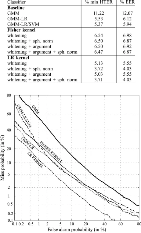
Fig. 3. DET curves of the GMM, GMM-LR, GMM-LR/SVM, Fisher kernel SVM and spherically normalized LR kernel SVM systems for text-independent speaker verification on PolyVar.
and 94 800, respectively, with an additional dimension for each if the argument is included.
The high score-space dimensionalities, particularly that of the LR kernel, causes computational problems for SVM optimiza-tion. We addressed this problem by whitening the score-vectors to zero-mean and unit diagonal variance (Section IV-C.1), and spherically normalizing them using (36). Since the vectors are whitened, setting the spherical normalization parameter to one will spread the data over a reasonably large portion of the hy-persphere. Each of the four kernels itemized above were trained with and without spherical normalization.
Classification in the score-space was carried out using linear SVMs. A static RBF or polynomial kernel could be used to make nonlinear decision boundaries in score-space. However, since the dimensionality of the score-space is significantly higher than
the number of training vectors, the classification problem is lin-early separable and nonlinear boundaries are unnecessary. Also, since the problem is known to be linearly separable, the regu-larization parameter [ in (10) or (15)] was set to infinity (i.e., the formulation for an SVM that maximizes the margin when the data is linearly separable was used). To give an indication of the value of the regularization parameter that should be used if more regularization were needed, the Lagrange multipliers in the spherically normalized likelihood ratio score-space kernel SVMs had a mean about 0.25 and an average maximum value of about 4.
We evaluated the results of our experiments using equal error rate (EER) and minimum HTER, and the results of the various systems are summarized in Table II. Scores such as EER and minimum HTER reflect performance at a single operating point on the detection error tradeoff (DET) curve; Fig. 3 uses DET curves to show the performance of the baseline systems and the SVM approaches at all operating points on PolyVar.
The GMM baseline from which the Fisher kernel is de-rived yielded 12.07% average EER. The Fisher kernel with whitening, but without spherical normalization or augmen-tation with the score-argument, reduced the average EER to 6.98%, a relative reduction of 42%. The application of spherical normalization and augmentation of the score-operator with the argument both reduced the EER but insignificantly (less than 2% relative). However, despite the improvement that the SVM imparted to the GMM system, the EER of the GMM-LR system was a further 11% lower relative to the spherically normalized Fisher kernel.
The basic LR kernel, without spherical normalization, re-duces the EER to 5.55%, relative reductions of 9% compared with the LR system and 7% compared with the GMM-LR/SVM system of [16]. Spherical normalization reduced the EER to 4.03%, a further relative reduction of 27% and an overall relative reduction of 34% compared with the GMM-LR system. Spherically normalizing the LR kernel resulted in a greater error reduction compared with applying the same normalization to the Fisher kernel. The dimension of the likelihood ratio score-space is six times larger than that of the likelihood score-space due to the inclusion of the world model, hence the Hessian computed from the LR kernel is more likely to be ill-conditioned. As was observed with the Fisher kernel, augmenting the kernel with the score-argument had a negligible effect.
Fig. 3 shows the DET curves of the LR, GMM-LR/SVM and spherically normalized LR kernel systems. It can be seen that the LR kernel results in a lower miss probability at all false alarm probabilities—in contrast to the GMM-LR/SVM system which has evidently optimized the parameters for a particular set of operating points (corresponding to EER and minimum HTER) at the expense of other points. At low false alarm probabilities, the LR kernel reduces the miss probability by over 20% compared to the GMM-LR system: when the prob-ability of misclassifying an impostor is 0.1%, the GMM-LR baseline has a probability of 45.5% of rejecting a client but the LR kernel SVM has a lower probability of 35.5%.
210 IEEE TRANSACTIONS ON SPEECH AND AUDIO PROCESSING, VOL. 13, NO. 2, MARCH 2005
represented by a single resultant vector , defined by (11). Thus, the number of parameters required per speaker is about four times that of the underlying client and world generative models: the lengths of and the mean and diagonal co-variance vectors, for whitening the score-space, plus the total number of client and world GMM parameters, plus one for the SVM bias.
VI. CONCLUSION
This paper has presented and evaluated a text-independent speaker verification system based on SVMs. The SVMs use the score-space kernels approach, which subsumes the Fisher kernel, to provide direct classification of whole sequences. Two score-space kernels were examined: the Fisher (likelihood score-space) kernel and the likelihood ratio score-space kernel. The Fisher kernel exploits one generative model (that of the client speaker) to map variable length sequences onto a single vector of fixed length, while the likelihood ratio kernel exploits two models (the client model and a world model).
Mapping to a fixed-length representation allows sequences of different durations to be compared and classified directly using traditional machine learning approaches. However, the score-space representation exists in a high-dimension score-space such that most classification strategies will suffer parameterization dif-ficulties. Fortunately, SVMs are well suited to this task and have the advantage of permitting discriminant analysis between whole sequences unlike, for example, HMMs, which only allow discriminant analysis between frames.
In order for the SVM to classify the score-space represen-tation effectively, two normalization steps were necessary: a whitening step, which normalizes the components of the score-space to zero mean and unit variance, and spherical normaliza-tion, which tackles the variability in the dynamic range of ele-ments in the Hessian associated with SVM optimization.
The PolyVar database was used in our evaluation. Compared to the GMM likelihood ratio baseline, the SVM approach without the use of spherical normalization reduced the average equal error rate by a relative amount of 9%. Spherical normal-ization enabled a much greater 34% relative reduction in the average equal error rate.
REFERENCES
[1] G. Doddington, M. Przybocki, A. Martin, and D. Reynolds, “The NIST speaker recognition evaluation—Overview, methodology, systems, re-sults, perspective,”Speech Commun., vol. 31, no. 2–3, pp. 225–254, 2000.
[2] D. A. Reynolds, “Speaker identification and verification using Gaussian mixture speaker models,”Speech Commun., vol. 17, pp. 91–108, 1995. [3] V. N. Vapnik,Statistical Learning Theory. New York: Wiley, 1998. [4] C. J. C. Burges, “A tutorial on support vector machines for pattern
recog-nition,”Data Mining and Knowl. Discov., vol. 2, no. 2, pp. 1–47, 1998. [5] M. Schmidt and H. Gish, “Speaker identification via support vector
clas-sifiers,” inProc. ICASSP, vol. 1, 1996, pp. 105–108.
[6] N. Smith, M. Gales, and M. Niranjan. (2001) Data-Dependent Kernels in SVM Classification of Speech Patterns. Engineering Dept., Cambridge Univ., Cambridge, U.K.. [Online]. Available: http://svr-www.eng.cam.ac.uk/~nds1002
[7] T. S. Jaakkola and D. Haussler, “Exploiting generative models in dis-criminative classifiers,” inAdvances in Neural Information Processing Systems 11, M. S. Kearns, S. A. Solla, and D. A. Cohn, Eds. Cam-bridge, U.K.: MIT Press, 1998.
[8] S. Fine, J. Navrátil, and R. A. Gopinath, “A hybrid GMM/SVM ap-proach to speaker identification,” inProc. ICASSP, vol. 1, 2001, pp. 417–420.
[9] L. Quan and S. Bengio, “Hybrid Generative-Discriminative Models for Speech and Speaker Recognition,”, Tech. Rep. IDIAP-RR 02-06, IDIAP, 2002.
[10] V. Wan and S. Renals, “Evaluation of kernel methods for speaker verifi-cation and identifiverifi-cation,” inProc. ICASSP, vol. 1, 2002, pp. 669–672. [11] V. Wan and W. M. Campbell, “Support vector machines for speaker
ver-ification and identver-ification,” inProc. Neural Networks for Signal Pro-cessing X, 2000, pp. 775–784.
[12] G. Chollet, J. L. Cochard, A. Constantinescu, C. Jaboulet, and P. Langlais, Swiss French Polyphone and PolyVar: Telephone Speech Databases to Model Inter- and Intra-Speaker Variability, J. Nerbonne, Ed: Linguistic Databases, 1997, pp. 117–135.
[13] A. P. Dempster, M. Laird, and D. B. Rubin, “Maximum likelihood from incomplete data via the EM algorithm,”J. Roy. Statist. Soc., pp. 1–39, 1977.
[14] R. A. Redner and H. F. Walker, “Mixture densities, maximum likelihood and the EM algorithm,” inSIAM Rev., vol. 26, 1984, pp. 195–202. [15] D. A. Reynolds, “A Gaussian Mixture Modeling Approach to
Text-In-dependent Speaker Identification,” Ph.D. dissertation, Georgia Inst. Technol., Atlanta, GA, 1992.
[16] S. Bengio and J. Mariéthoz, “Learning the decision function for speaker verification,” inProc. ICASSP, vol. 1, 2001, pp. 425–428.
[17] R. Courant and D. Hilbert,Methods of Mathematical Physics. New York: Wiley Interscience, 1953.
[18] N. Smith and M. J. F. Gales, “Using SVM’s and discriminative models for speech recognition,” inProc. ICASSP, vol. 1, 2002, pp. 77–80. [19] N. Smith and M. Gales, “Speech recognition using SVMs,” inAdvances
in Neural Information Processing Systems. Cambridge, MA: MIT Press, 2002, vol. 14.
[20] V. Wan, “Speaker Verification Using Support Vector Machines,” Ph.D. dissertation, Univ. Sheffield, Sheffield, U.K., 2003.
[21] J. P. Campbell Jr, “Testing with the YOHO CD-ROM voice verification corpus,” inProc. ICASSP, vol. 1, 1995, pp. 341–344.
[22] F. Bimbot, M. Blomberg, and L. Boves, “An overview of the PICASSO project research activities in speaker verification for telephone applica-tions,” inProc. Eurospeech, vol. 5, 1999, pp. 1963–1966.
[23] K. Koumpis, S. Renals, and M. Niranjan, “Extractive summarization of voicemail using lexical and prosodic feature subset selection,” inProc. Eurospeech, vol. 4, 2001, pp. 2377–2380.
Vincent Wanreceived the B.A. degree in physics from the University of Oxford, Oxford, U.K., in 1997 and the Ph.D. degree in speaker verification and support vector machines from the University of Sheffield, Sheffield, U.K., in 2003.
In 1998 and 1999, he worked on hybrid speech recognition at the University of Sheffield, then spent 2000 working at the Motorola Human Interface Labs, Palo Alto, CA, on speech and handwriting recogni-tion. He is presently holding a postdoctoral position in the Department of Computer Science, University of Sheffield. His interests include machine learning, biometrics, and speech pro-cessing.
Steve Renals(M’91) received the B.Sc. degree in chemistry from the University of Sheffield, Sheffield, U.K., the M.Sc. degree in artificial intelligence, and the Ph.D. degree in neural network, both from the University of Edinburgh, Edinburgh, U.K.