Mediated Population Protocols
I,IIOthon Michaila,b,∗, Ioannis Chatzigiannakisa,b, Paul G. Spirakisa,b aResearch Academic Computer Technology Institute (RACTI), Patras, Greece bComputer Engineering and Informatics Department (CEID), University of Patras
Abstract
We extend here the Population Protocol (PP) model of Angluinet al. [2004,2006] in order to model more powerful networks of resource-limited agents that are possibly mobile. The main feature of our extended model, called theMediated Population Protocol(MPP) model, is to allow the edges of the interaction graph to have states that belong to a constant-size set. We then allow the protocol rules for pairwise interactions to modify the corresponding edge state. The descriptions of our protocols preserve both theuniformityandanonymity prop-erties of PPs, that is, they do not depend on the size of the population and do not use unique identifiers. We focus on the computational power of the MPP model on complete interaction graphs and initially identical edges. We provide the following exact characterization of the class MPS of stably computable predicates: A predicate is inMPSiff it is symmetric and is inNSPACE(n2).
Keywords:
population protocol, diffuse computation, finite-state agent, intermittent communication, stable computation, passive mobility
1. Introduction - Population Protocols
Theoretical models for Wireless Sensor Networks (WSNs) have received great attention over the past few years, mainly because they constitute an abstract but yet formal and precise method for understanding the limitations and capabili-ties of this widely applicable new technology. ThePopulation Protocol model [AAD+04, AAD+06] was designed to represent a special category of WSNs which is mainly identified by two distinctive characteristics: each sensor node
IThis work has been partially supported by the ICT Programme of the European Union under contract number ICT-2008-215270 (FRONTS).
IISome preliminary versions of the results in this paper have also appeared in [CMS09a, CMN+10a, CMS09b].
∗Corresponding author (Telephone number: +30 2610 960200, Fax number: +30 2610
960490, Postal Address: Research Academic Computer Technology Institute (RACTI), N. Kazantzaki Str., Patras University Campus, Rio, P.O. Box 1382, 26500, Greece).
is an extremely limited computational device and all nodes move according to some mobility pattern over which they have totally no control.
One reason for studying extremely limited computational devices is that in many real WSNs’ application scenarios having limited resources is inevitable. For example, power supply limitations may render strong computational devices useless due to short lifetime. In other applications, mote’s size is an important constraint that thoroughly determines the computational limitations. The other reason is that the population protocol model constitutes the starting point of a brand new area of research and in order to provide a clear understanding and foundation of the laws and the inherent properties of the studied systems it ought to be minimalistic. In terms of computational characterization each node is simply a finite-state machine additionaly equipped with sensing and communication capabilities and is usually called anagent. Apopulation is the collection of all agents that constitute the distributed computational system. Two outstanding properties of population protocols is that they areuniformand
anonymous. The so calleduniformity property requires that the descriptions of the protocols are independent of the population size and theanonymity property
that there is no room in the state of an agent to store a unique identifier1. As already mentioned, another prominent characteristic of population pro-tocols is the total inability of the computational devices to control or predict their underlying mobility pattern. Their movement is usually the result of some unstable environment, like water flow or wind, or the natural mobility of their carriers, like in the now canonical example in which each bird in a flock is equipped with such an agent and the birds naturally move, and is known as
passive mobility. The agents interact in pairs and are absolutely incapable of knowing the next pair in the interaction sequence. This inherent nondetermin-ism of the interaction pattern is modeled by anadversary whose job is to select interactions. The adversary is a black-box and the only restriction imposed is that it has to befair so that it does not forever partition the population into noncommunicating clusters and guaranteeing that interactions cannot follow some inconvenient periodicity. The above characteristics render the study of population protocols a non-trivial task.
As expected, due to the minimalistic nature of the population protocol model, the class of computable predicates was proven [AAD+06, AAER07] to be fairly small: it is the class ofsemilinear predicates [GS66] (or, equivalently, all predicates definable by first-order logical formulas inPresburger arithmetic
[Pre29]), which does not include multiplication of variables, exponentiations, and many other important and natural operations on input variables. More-over, we only know how to transform any protocol that computes a function in the failure-free model into a protocol that can tolerate O(1) crash failures. 2 However, this requires some inevitable weakening of the problem
specifica-1Throughout the text we abbreviate the word “identifier” by “id” and we use “uid” when
we want to emphasize the fact that the identifier is “unique”.
tion. This result is due to Delporte-Gallet et al. [DGFGR06]. Additionally, Guerraoui and Ruppert [GR09] showed that any function computable by a pop-ulation protocol tolerating one Byzantine agent is trivial. On the other hand, Angluin, Aspnes, and Eisenstat [AAE08b] described a population protocol that computes majority toleratingO(√n) Byzantine failures. However, that protocol was designed for a much more restricted setting, where the scheduler chooses the next interaction randomly and uniformly (see the probabilistic population protocols discussion in Section 2.1).
2. Enhancing the Model
The work of Angluinet al. shed light and opened the way towards a brand new and very promising direction. The lack of control over the interaction pattern, as well as its inherent nondeterminism, gave rise to a variety of new theoretical models for WSNs. Those models draw most of their beauty precisely from their inability to organize interactions in a convenient and predetermined way. In fact, the population protocol model was the minimalistic starting-point of this area of research. Most efforts are now towards strengthening the model of Angluinet al. with extra realistic and implementable assumptions, in order to gain more computational power and/or speed-up the time to convergence and/or improve fault-tolerance. Several promising attempts have appeared towards this direction. In each case, the model enhancement is accompanied by a logical question: What is exactly the class of predicates computable by the new model? One idea is to allow some heterogeneity in the model, so that some agents have more computational power than others. For example, a base station can be an additional part of the network with which the agents are allowed to communicate [BCM+07].
Another extension was the Community Protocol model of Guerraoui and Ruppert [GR09] in which the agents are equipped with read-only uids picked from an infinite set of ids. Moreover, each agent can store up to a constant number of other agents’ ids. In this model, agents are only allowed to compare ids, that is, no other operation on ids is permitted. The community protocol model was proven to be extremely strong: the corresponding class consists of all symmetric predicates inNSPACE(nlogn), wherenis the community size. The proof was based on a simulation of a modified version of Sch¨onhage’s (Non-deterministic)Storage Modification Machine. It was additionally shown that if faults cannot alter the uids and if some necessary preconditions are satisfied, then community protocols can tolerateO(1) Byzantine agents.
ThePassively mobile Machines (PM) model [CMN+10c, CMN+10d] made the assumption that each agent instead of being an automaton is a Turing
chine3with unbounded memory. Then the authors studied computations upper-bounded by plausible space limitations. They focused on complete interaction graphs and defined the complexity classes PMSPACE(f(n)) parametrically, consisting of all predicates that are stably computable by some PM protocol that usesO(f(n)) memory on each agent. That work arrived at an exact char-acterization of the classesPMSPACE(f(n)) when f(n) = Ω(logn): they are precisely the classes of all symmetric predicates in NSPACE(nf(n)). Also the computability of the PM model when the protocols use o(log logn) space per machine was explored and was proved that SEM = PMSPACE(f(n)) whenf(n) =o(log logn), whereSEMdenotes the class of the semilinear pred-icates. In fact, it was proved that this bound acts as a threshold, so that
SEM(PMSPACE(f(n)) whenf(n) =O(log logn).
This work proposes another extension of the population protocol model which seems to be of its own theoretical interest. The main additional fea-ture of the new model is that the communication links are capable of storing limited information. We are mainly interested in the model’s computational capabilities and study it on a purely theoretical ground. We call our model the
Mediated Population Protocol (MPP) model.
2.1. Other Previous Work
Much work concerning the population protocol model has been devoted to establishing that the class of computable predicates is precisely the class of
semilinear predicates [AAD+04, AAD+06, AAE06, AAER07]. Moreover, in [AAD+04, AAD+06], theprobabilistic population protocol model was proposed, in which the scheduler selects randomly and uniformly the next interaction pair. Some work has concentrated on performance, supported by this random schedul-ing assumption (see e.g. [AAE08a]). [CDF+09] proposed a generic definition of probabilistic schedulers and a collection of new fair schedulers, and revealed the need for the protocols to adapt when natural modifications of the mobil-ity pattern occur. [BCK+09, CS08] considered a huge population hypothesis (population going to infinity), and studied the dynamics, stability and com-putational power of probabilistic population protocols by exploiting the tools of continuous nonlinear dynamics. Moreover, several extensions of the basic model have been proposed in order to more accurately reflect the requirements of practical systems. In [AAC+05], Angluin et al. studied what properties of restricted interaction graphs are stably computable by the population protocol model, gave protocols for some of them, and proposed an extension of the model withstabilizing inputs in order to resolve the resistance of population protocols to composability. Some other works incorporated agent failures [DGFGR06]. Recently, Bournezet al. [BCCK08] investigated the possibility of studying pop-ulation protocols via game-theoretic approaches. For some introductory texts to the subject of population protocols see [AR07, Spi10, MCS10] and for a survey
3As common in the CS literature, we abbreviate a Turing Machine by TM and by NTM
mostly based on preliminary results of this work see [CMS09b]. Finally, the
Static Synchronous Sensor Field (SSSF) [ADGS09, ASS10] is a very promising recently proposed model that addresses networks of tiny heterogeneous compu-tational devices and additionally allows processing over constant flows (streams) of data originating from the environment. The latter feature is totally absent from the models discussed so far and is required by various sensing problems. See [ACD+11] for a joint survey on population-protocol-like models and static synchronous sensor fields.
3. Our Results - Roadmap
Section 4 provides a formal definition of the MPP model. Section 5 fo-cuses on the computational power of the model by studying what predicates on input assignments are stably computable in the fully symmetric case, in which the interaction graph is complete and all edges are initially in a common state. First Section 5.1 proves that the MPP model is strictly stronger than the population protocol model by showing that the former can stably compute a non-semilinear predicate. Then in Section 5.2 it is shown that the MPP model can turn itself into a deterministic TM of linear space. Section 5.3 first ex-tends the techniques developed in Section 5.2 to show that the MPP model can simulate a NTM of O(n2) space and then, by showing that the inverse inclu-sion also holds, it establishes the following exact characterization of the class of computable predicates by the MPP model: it is precisely the class of sym-metric predicates inNSPACE(n2). Thus, unexpectedly, while preserving both
uniformityandanonymity, the MPP model turns out to be an extremely pow-erful enhancement: it dramatically extends the class of computable predicates, from semilinear predicates to all symmetric predicates computable by a NTM in
O(n2) space. Section 6 concludes and discusses some promising future research directions.
4. The Mediated Population Protocols: A Formal Model
4.1. Formal Definition
Definition 1. A Mediated Population Protocol (MPP) is a 7-tuple (X, Y, Q, S, I, O, δ), whereX,Y,Q, andS are all finite sets and
1. X is the input alphabet,
2. Y is the output alphabet,
3. Qis the set of agent states,
4. S is the set of edge states,
5. I:X →Qis the input function,
6. O:Q→Y is the output function,
7. δ:Q×Q×S→Q×Q×S is the transition function.
An interaction graph is a (usually directed) graph G = (V, E), where V
specifies the set of agents (also called a population) andE the permissible in-teractions between them; that is, (u, v) ∈ E indicates the possibility of an interaction between agents u and v, in which uis the initiator and v the re-sponder. Throughout this article we use the lettersnandmto denote |V|and
|E|, respectively. Agraph universe (orgraph family)U is any set of interaction graphs. Unless otherwise stated, we assume that the graph universes under con-sideration consist of directed interaction graphs without self-loops and multiple edges. We denote byGconthe graph universe consisting of all weakly connected interaction graphs of any finite number of nodes greater or equal to 2. Given a fixed graph universeU, a MPPAruns on the nodes of an interaction graph
G= (V, E)∈ U.
In the most general setting, each agent initially senses its environment, as a response to a global start signal, and receives an input symbol fromX. Then all agents concurrently apply the input function to their input symbols and obtain their initial state (in this way theinitial configurationof the system is formed). Each edge is initially in one state fromS as specified by someedge initialization function ι : E → S, which is not part of the protocol but generally models some preprocessing on the network that has taken place before the protocol’s execution.
Anetwork configuration, or simply aconfiguration, is a mappingC:V∪E→ Q∪S specifying the state of each agent in the population and each edge in the set of permissible interactions. LetC andC0 be configurations, and letu,υ be distinct agents. We say that C goes to C0 via encounter e = (u, υ), denoted
C→e C0, if
C0(u) =δ1(C(u), C(υ), C(e))
C0(υ) =δ2(C(u), C(υ), C(e))
C0(e) =δ3(C(u), C(υ), C(e))
C0(z) =C(z), for allz∈(V − {u, υ})∪(E− {e}),
that is,C0is the result of the interaction of the pair (u, υ) under configurationC
and is the same asC except for the fact that the states ofu,υ, and (u, υ) have been updated according toδ1,δ2, andδ3, respectively. We say thatCcan go to
C0 in one step, denotedC→C0, ifC→e C0for some encountere∈E. We write
C→∗ C0 if there is a sequence of configurationsC=C0, C1, . . . , Ct=C0, such
that Ci →Ci+1 for all i, 0 ≤i < t, in which case we say that C0 isreachable fromC.
on the adversary to ensure the protocol makes progress. An infinite execution is fair if for every pair of configurations C and C0 such that C → C0, if C
occurs infinitely often in the execution then so doesC0. An adversary scheduler is fair if it always leads to fair executions. A computation is an infinite fair execution. An interaction between two agents is calledeffective if at least one of the initiator’s, the responder’s, and the edge’s states is modified (that is, if
C,C0 are the configurations before and after the interaction, respectively, then
C0 6=C). Similarly, a transition (a, b, c)→(a0, b0, c0) is called effective ifa06=a, orb0 6=b, orc06=c.
Note that the mediated population protocol modelpreserves both uniformity and anonymityproperties of population protocols. As a result, any MPP’scode
is ofconstant size, thus, can be stored in each agent (device) of the population and, additionally, there is not enough room in the states of the agents and the edges to store uids. Nevertheless, as we shall see, the MPP model can handle far more complicated computations than the population protocol model.
4.2. Stable Computation
The input (also called aninput assignment) to a MPP is anyx=σ1σ2. . .
σn∈X∗such thatn=|V|.4 In particular, by assuming an ordering overV, the
input to agentiis the symbolσi, for alli, 1≤i≤n. Letp:X∗→ {0,1}be some
predicate overX∗. pis calledsymmetric if for everyx=σ1σ2. . . σn∈X∗ and
any permutation functionπ:{1,2, . . . , n} → {1,2, . . . , n}, it holds that p(x) =
p(σπ(1)σπ(2). . . σπ(n)) (in words, permuting the input symbols does not affect the predicate’s outcome). Similarly, a languageL⊆X∗ is called symmetric if
x = σ1σ2. . . σn ∈ L implies σπ(1)σπ(2). . . σπ(n) ∈ L for all π. Any language
L⊆X∗ corresponds to a unique predicatepL defined aspL(x) = 1 iffx∈L. It
is easy to see thatL is symmetric iffpL is symmetric. Due to this bijection we
use the termsymmetric predicate for both predicates and languages.
Like population protocols, MPPs do not halt. Instead a protocol is required tostabilize, in the sense that it reaches a point after which the output of every agent will remain unchanged. A configurationCis calledoutput stable if for ev-ery configurationC0that is reachable fromCit holds thatO(C0(u)) =O(C(u)) for all u∈ V, where O(C(u)) is the output of agent uunder configurationC. In simple words, if an output stable configuration is ever reached, no agent will change its output in any subsequent step and no matter how the computation proceeds thereafter.
A predicatepoverX∗is said to bestably computableby the MPP model in a graph universeU, if there exists a MPPAsuch that for any input assignment
x∈ X∗ and any G = (V, E) ∈ U s.t. |V| =|x|, any computation of A onG
beginning from the initial configuration corresponding to xeventually (i.e. in a finite number of steps) reaches an output stable configuration in which all agents outputp(x).
4The truth is that we consider only graphs with at least 2 nodes, since smaller graphs do
A configuration C is called state stable if for every configuration C0 s.t.
C→∗ C0 it holds thatC0 =C. We say that a protocol Ahasstabilizing states
if every computation ofAeventually reaches a state stable configuration; that is, the states of all agents eventually stop changing. Note that any protocol that state-stabilizes alsooutput-stabilizes, but the inverse is not generally true (stabilizing states is a stronger requirement).
In some cases, a protocol, instead of stably computing a predicate p, may provide some different sort of guarantee. For example, whenever runs on some
x∈X∗ such thatp(x) = 1, it may forever remain to configurations where at least one agent is in statea, and whenever p(x) = 0 it may forever remain to configurations where no agent is in state a. To formalize this, we say that a MPPAguaranteest:Q∗→ {0,1}w.r.t. p:X∗→ {0,1}in a graph universeU if, for any input assignmentx∈X∗ and anyG= (V, E)∈ U s.t. |V|=|x|, any computation ofA onGbeginning from the initial configuration corresponding toxeventually reaches a configurationC, s.t. for allC0, whereC→∗ C0, it holds thatt(C0) =t(C) =p(x).5
5. Predicates on Input Assignments
We assume here that the interaction graph is complete and that all edges are initially in a common states0, that is, the universe is{G|Gis complete} andι(e) =s0for alle∈E. Call this for the sake of simplicity the SMPP model (‘S’ standing for “Symmetric”). We are interested in the computational power of the SMPP model. In particular, we provide an exact characterization of the predicates on input assignments that are stably computable.
Definition 2. Let MPS (standing for “Mediated Predicates in the fully Sym-metric case” 6) be the class of all stably computable predicates by the SMPP model.
Lemma 1. All predicates in MPSare symmetric.
Proof. Take any p ∈ MPSand let A be the SMPP that stably computes it. Take also any input assignment x = σ1σ2. . . σn and let π : V → V be any
permutation of V = {1,2, . . . , n}. Now consider the input assignment x0 =
σπ(1)σπ(2). . . σπ(n), which is a permutation ofx. Take any fair, w.r.t. A, infinite interaction sequence7e1, e2, . . ., whereei ∈E, and replace eachei= (j, k) with
(π(j), π(k)) to obtain a new infinite interaction sequence, which is well defined due to the fact that the interaction graph is complete. Now consider the two infinite executions of A that correspond to the two interaction sequences on inputs x and x0, respectively. Obviously, x0w = xπ(w), so that for the initial
configurationsC00 andC0we have thatC00(w) =C0(π(w)) for all agentsw∈V.
5Note that by assuming an ordering onV we can define configurations as strings fromQ∗,
as we did for the input assignments at the beginning of this subsection.
Moreover, we have initially that C00(j, k) = C0(π(j), π(k)) for all (j, k) ∈ E, which holds trivially since all edges are initially ins0. Assume that the above holds for some interaction stepi, that is,Ci0(w) =Ci(π(w)) for allw∈V and Ci0(j, k) = Ci(π(j), π(k)) for all (j, k)∈E. It is not hard to see that the same
must hold for step i+ 1, consequently both infinite executions pass in each step through the same multiset of states. This together with the fact that one execution is fair implies that the other must also be fair. So, we have obtained two computations ofAon inputsxandx0, respectively, that forever provide the same multisets of output symbols. Now, the fact thatpis stably computable implies thatp(x) =p(x0), which in turn implies thatphas to be symmetric.
Throughout the text, we useSSPACE(f(n)) andSNSPACE(f(n)) to de-note SPACE(f(n))’s and NSPACE(f(n))’s restrictions to symmetric predi-cates, respectively andSEMto denote the class of semilinear predicates.
In the rest of this article, we build the machinery required to arrive at the exact characterization ofMPSthat is captured by Theorem 1.
Theorem 1. MPS=SNSPACE(n2).
Proof. One direction follows from Theorem 10 and the inverse direction from Corollary 2.
We begin by providing an abstract proof idea of the above Theorem that briefly discusses most techniques that we develop throughout the rest of the article. This is done for the sake of clarity and readability of the results that follow.
Proof Idea. The “only if” part is easy. Any predicate in MPS is obviously symmetric and additionally we can perform inO(n2) space a nondeterministic search on the transition graph of the SMPP that stably computes the predicate. The sufficiency of the conditions is somewhat more complicated. We have to show that for all symmetric languages L ∈ NSPACE(n2) there exists a SMPP that stably computes pL, defined as pL(x) = 1 iff x ∈ L. The idea is
to organize the agents into a spanning pseudo-path subgraph of the interac-tion graph (pseudo-path graphs are defined in the beginning Secinterac-tion 5.2). To do that, the agents begin to form small pseudo-path graphs that in the sequel are merged together and are expanded to isolated nodes. When this process ends, the edges of the spanning pseudo-path graph will be active and all other
input that is maintained throughout the computation. The final reinitialization happens when the spanning pseudo-path graph is formed an then the simulation is executed correctly.
5.1. MPSis a Proper Superset ofSEM
In this section, we provide a first inclusion (in fact, a lower bound) forM P S. By combining Theorems 2 and 3, we get in Corollary 1 that the non-semilinear predicate (Nc = Na ·Nb) belongs to MPS, where Nσ denotes the number
of agents that initially obtain the input symbol σ and ‘·’ denotes standard multiplication. This (due to the fact that population protocols cannot handle multiplication of variables [AAE06]) establishes the following separation: MPS is a proper superset ofSEM(which is captured by Theorem 4).
Protocol 1VarProduct
1: X ={a, b, c} 2: Y ={0,1} 3: Q={a,a, b, c,˙ ¯c} 4: S={0,1}
5: I(σ) =σ, for allσ∈X
6: O(a) =O(b) =O(¯c) = 1 andO(c) =O( ˙a) = 0
7: δ: (a, b,0)→( ˙a, b,1), (c,a,˙ 0)→(¯c, a,0), ( ˙a, c,0)→(a,¯c,0)
8: // All transitions that do not appear have no effect, e.g. δ(a, b,1) = (a, b,1)
Theorem 2. Protocol VarProduct (see Protocol 1) provides w.r.t. predicate
(Nc =Na·Nb)the following semilinear guarantee:
• IfNc 6=Na·Nb then at least one agent remains in one of the statesa˙ and c.
• If Nc=Na·Nb then no agent remains in these states.
Proof. First of all, we notice that in a complete directed interaction graph,
Na·Nb equals to the number of links leading from agents in stateato agents
in stateb. The main idea is that we should erase a number ofc’s equal to the number of a’s times the number of b’s. That is, for each a we should erase b c’s. In the population protocol model, the impossibility for computing such a predicate comes from the fact that there is no way for an agent being w.l.o.g. in stateato be able to say that it has already counted a specific agent in stateb. If e.g. Na=Nb=Nc =O(n), then it is impossible in the population protocol
model for eachbto be able to remember alla’s that have already counted it. On the other hand, in the SMPP model this is resolved easily. It is easy to see that when at least one ofNa, Nb, andNc is equal to zero, then in all such
cases, except for the case whereNc = 0, Na 6= 0 andNb 6= 0, no computation
while the second and third rules cannot be applied (since Nc always remains
zero) and, thus, at least one agent goes to state ˙awithout being able to leave from it. Noticing thatNa·Nb 6= 0 it is obvious that in this case a ˙acorrectly
remains inV arP roduct’s computation.
The interesting case is when allNa,NbandNcare not equal to zero (in fact
they are greater than zero since theNq’s are always non-negative). Recall that
all edges are initially in their initial common state 0. The protocol proceeds as follows. When an agent in statea interacts as the initiator with an agent in stateb, then the initiator goes to ˙a and the corresponding edge goes to state 1. The modification in the state of the edge defining this specific ordered pair (a, b) is all the protocol needs to “remember” in order not to count the same pair again. When an agent in statec interacts with an agent in state ˙a, then
c is erased by becoming ¯c and ˙areturns to its natural operation by becoming
aagain. The crucial point is to notice that the protocol tries to erase Na·Nb
agents in statec. IfNc =Na·Nb, then it will eventually manage to do it and
at that point no agent will be in one of the states ˙a and c and, moreover, no agent will be able to go again to one of these states. Thus, in this case, the protocol guarantees that eventually no agent remains in one of the states ˙aand
c. If Nc < Na·Nb then eventually at least one agent will remain to state ˙a,
while there will be no unerased agent in statec to be able to turn it again to statea. Finally, whenNc > Na·Nb some agents in statecwill keep their state,
since there will be no unvisited (a, b) pair to erase any of thosec’s. Thus, when
Nc6=Na·Nb the protocol guarantees that at least one agent remains in one of
the states ˙aandcand this completes the proof.
Remark 1. It is easy to see that Protocol VarProduct has stabilizing states.
Note that Theorem 2 alone does not complete the separation of SEMand
MPS. The reason is that it does not show that the SMPP model stably com-putes (Nc=Na·Nb); what it truly shows is that whenever the predicate is true
a state stable configuration is reached for which another predicatet on config-urations becomes true, and whenever it is false a state stable configuration is reached for whichtis also false. In fact, there is a way to exploit the guarantee and the stabilizing states in order to achieve the separation. This is captured by the following general composition theorem holding also for non-complete interaction graphs.
Theorem 3. LetGbe some family of directed and connected interaction graphs. If there exists a MPP A with stabilizing states that, in G, guarantees w.r.t. a predicate p a semilinear predicate t, then p is stably computable by the MPP model inG.
Proof. We show that Acan be composed with a provably existing protocol B that stably computestto give a new MPPCsatisfying the following properties:
• C is formed by the composition ofAandB,
• its output isB’s output, and
• C stably computesp(i.e. all agents agree on the correct output) inG.
ProtocolAhas stabilizing states and provides a guaranteetwhich is a semi-linear predicate onA’s configurations. LetXA=X be the input alphabet ofA,
QA the set ofA’s states,δAthe transition function ofA, and similarly for any other component ofA. We will use the indexesB andC, for the corresponding components of the other two protocols.
Since predicatetis semilinear, according to a result in [AAC+05], there is a population protocol B0 that stably computest with stabilizing inputs in Gcon. Note thatG ⊆ Gcon, so any predicate stably computable (both with or without stabilizing inputs) in Gcon is also stably computable in G. In fact, the same protocol B0 stably computes t with stabilizing inputs in G. Moreover, there also exists a mediated population protocol B (the one that is the same as B0 but simply ignores the additional components of the new model) that stably computest with stabilizing inputs inG. Note that the input alphabet of B is
XB =QA, and its transition function is of the formδB : (QA×QB)×(QA× QB) → QB×QB, since there is no need to specify edge states (formally we should, but the protocol ignores them). In fact,QA also plays the role of B’s inputs that eventually stabilize.
We define a mediated population protocol C as follows: XC = XA, YC =
YB = {0,1}, QC = QA×QB, IC : XA → QC defined as IC(x) = (IA(x), iB) for all x ∈ QC, where iB ∈ QB is the initial state of protocol B, SC = SA,
OC(a, b) = OB(b), for all q = (a, b) ∈ QC, and finally its transition function
δC :QC×QC×SC →QC×QC×SC is defined as
δC((a, b),(a0, b0), s) = ((δA1(a, a0, s), δB1((a, b),(a0, b0))),
(δA2(a, a0, s), δB2((a, b),(a0, b0))), δA3(a, a0, s)),
where for δA(x, y, z) = (x0, y0, z0) (in A’s transition function), we have that
components ofC’s agent states eventually stabilize as a result of the fact that
A has stabilizing states, protocol B will eventually obtain stabilizing inputs, consequently will operate correctly, and will stably computetas if it had began computing onA’s state stable configuration. But, sincet provides the correct answer forp if applied on A’s state stable configuration, it is obvious that C must stably computepin G, and the theorem follows.
Corollary 1. The non-semilinear predicate (Nc=Na·Nb)belongs toMPS. Proof. The SMPP VarProduct has stabilizing states (Remark 1) and in the family of all complete directed interaction graphs guarantees w.r.t. (Nc=Na· Nb) a semilinear predicate (Theorem 2). Consequently, the requirements of
Theorem 3 are satisfied and (Nc=Na·Nb) is stably computable by the SMPP
model in the family of all complete directed interaction graphs.
Theorem 4. SEM(MPS.
Proof. Clearly, the population protocol model is a special case of the mediated population protocol model, therefore SEM ⊆ MPS and, by Corollary 1 to-gether with the fact that (Nc =Na·Nb) is non-semilinear, (Nc =Na·Nb)∈ MPS−SEM.
5.2. A Better Inclusion: SSPACE(n)⊆MPS
We are now going to establish a much better inclusion. In particular, we will show that any predicate inSSPACE(n) is also inMPS. In other words, the SMPP model is at least as strong as a linear space TM that computes symmetric predicates. We begin with some necessary definitions.
LetG= (V, E) be an interaction graph and letdG(u)≡ |{w∈V |(u, w)∈E
or (w, u)∈E}|denote the degree ofuw.r.t. G. Apseudo-path graphL= (K, A) is a directed graph either satisfying |K| = 1 and A =∅ or |K| >1, dL(u) = dL(v) = 1 for someu, v ∈K, anddL(w) = 2 for allw∈K− {u, v}. In words,
it is either an isolated node, which we call thetrivial pseudo-path graph, or a directed graph that becomes a path graph when the directions of the links are ignored. A pseudo-path subgraph of G is a pseudo-path graph L ⊆ G and is calledspanning ifK=V. LetCl(t) denote thelabel component of the state of t∈V ∪E under configurationC.
We say that a pseudo-path subgraph of Giscorrectly labeled under config-urationC, if it is trivial and its label isl with no active edges incident to it or if it is non-trivial and all the following conditions are satisfied:
1. Assume thatu, υ ∈K anddL(u) =dL(υ) = 1. These are the only nodes
inKwith degree 1. Then one ofuandυhas labelkt(non-leader endpoint)
and the other has either lt or lh (leader endpoint). The unique eu ∈ A
incident tou, where uhas w.l.o.g. labelkt, is an outgoing edge and the
unique eυ ∈ A incident to υ is outgoing if Cl(υ) = lt and incoming if Cl(υ) =lh.
3. For alla∈Ait holds thatCl(a)∈ {p, i}(active edges) and for alle∈E−A
such that e is incident to a node in K it holds that Cl(e) = 0 (inactive
edges).
4. Letυ=u1, u2, . . . , ur=ube the path from the leader to the non-leader
endpoint (resulting by ignoring the directions of the arcs inA). LetPL= {(ui, ui+1)|1 ≤i < r} be the corresponding directed path fromυ to u. Then for alla∈A∩PL it holds thatCl(a) =p(proper edges) and for all a0∈A−PL that Cl(a0) =i(inverse edges).
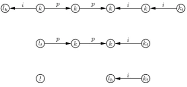
[image:14.595.210.399.262.350.2]See Figure 1 for some examples of correctly labeled pseudo-path subgraphs. The meaning and service of each label will become clear in the following discussion.
Figure 1: We assume that the above depicted graph, call itG, is complete. We have chosen not to draw the inactive edges for the sake of visibility. Therefore, all edges not appearing have label 0, that is, they are inactive. The top six nodes form a correctly labeled pseudo-path subgraph ofG. The reason is that the left endpoint has label lh, that is, it is a head
leader, the right endpoint has labelkt, that is, it is a tail non-leader (condition 1 satisfied),
all intermediate nodes are (simple) non-leaders (condition 2 satisfied), the edges that follow the direction from left to right have labelp, that is, they are proper, those that follow the direction from right to left have labeli, that is, they are inverse, and all other edges incident to these nodes (those that do not appear) are inactive (conditions 3 and 4 satisfied). Similarly, all other appearing graphs are pseudo-path subgraphs of the complete graphG. Note that the left node at the bottom that seems to be isolated, is in fact a node ofGwhose incident edges are all inactive. Moreover, it has labell, consequently it constitutes a trivial pseudo-path subgraph ofG.
We describe now a SMPP, called Spanning Process, that constructs a cor-rectly labeled spanning pseudo-path subgraph of any complete interaction graph
G. The correctness of the protocol is captured by Theorem 5. We provide a high level description of the protocol in order to avoid its many low-level details. All agents have initially labell, thought of as being simple leaders. All edges have label 0 and we think of them as being inactive, that is, not part of the pseudo-path subgraph to be constructed. An edge having labelpis interpreted as proper while an edge having label i is interpreted as inverse and both are additionally interpreted asactive, that is, part of the pseudo-path subgraph to be constructed. An agent with labelkis a (simple)non-leader, an agent withkt
is a non-leader that is additionally thetail of some pseudo-path subgraph (tail non-leader), an agent having label ltis a leader and a tail of some pseudo-path
subgraph (tail leader), and an agent having lh is a leader and a head of some
When two simple leaders interact through an inactive edge, the initiator becomes a tail non-leader, the responder becomes a head leader, and the edge becomes inverse. When a head leader interacts as the initiator with a simple leader via some inactive edge the initiator becomes a non-leader, the responder becomes a head leader, and the edge becomes inverse. When the simple leader is the initiator, the head leader is the responder, and the edge is again inactive, the initiator becomes a tail leader, the responder becomes a non-leader, and the edge becomes proper. When a tail leader interacts as the initiator with a simple leader via an inactive edge, the initiator becomes a non-leader, the responder becomes a head leader, and the edge becomes inverse. When the simple leader is the initiator, the tail leader is the responder, and the edge is again inactive, the initiator becomes a tail leader, the responder becomes a non-leader, and the edge becomes proper. These transitions can be formally summarized as follows: (l, l,0)→(kt, lh, i), (lh, l,0)→(k, lh, i), (l, lh,0)→(lt, k, p), (lt, l,0)→
(k, lh, i), and (l, lt,0)→(lt, k, p). In this manner, the agents become organized
in correctly labeled pseudo-path subgraphs (see again their definition and Figure 1).
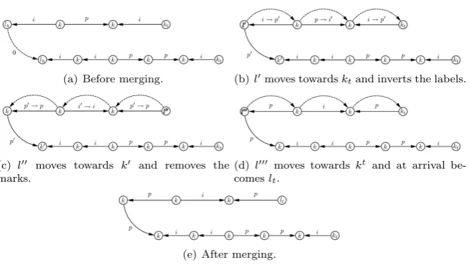
We now describe how two such pseudo-path graphs L1 and L2 are pieced together. Denote by l(L) ∈ V and by kt(L) ∈ V the leader and tail
non-leader endpoints of a correctly labeled pseudo-path graphL, respectively. When
l(L1) = uinteracts as the initiator with l(L2) = υ, through an inactive edge,
υ becomes a non-leader with a special mark, e.g. k0, the edge becomes proper with a special mark, andubecomes a leader having a special labell0indicating that this label will travel towardskt(L1) while making all proper edges that it meets inverse and all inverse edges proper. In order to know its direction, it marks each edge that it crosses. When it, finally, arrives at the endpoint, it takes to another special label and walks the same path in the inverse direction until it meetsυ again. This walk can be performed easily, without using the marks, because now all edges have correct labels. To diverge fromL1’s endpoint it simply follows the proper links as the initiator (moving from their tail to their head) and the inverse links as the responder (moving from their head to their tail) while erasing all marks left from its previous walk. When it reachesυ it erases its mark, making its labelk, and obtains another special label indicating that it again must walk towardskt(L1) for the last time, performing no other
operation this time. To do that, it follows the proper links as the responder (from their head to their tail) and the inverse links as the initiator (from their tail to their head). When it, finally, arrives atkt(L1) it becomes a normal tail leader and now it is easy to see thatL1andL2have been correctly merged into a common correctly labeled pseudo-path graph. See Figure 2 for a graphical step by step example. The correctness of this process, called themerging process, is captured by Lemma 2.
Lemma 2. When the leader endpoints of two distinct correctly labeled pseudo-path subgraphs of G, L1 = (K1, A1) and L2 = (K2, A2), interact via e ∈ E,
then, in a finite number of steps, L1 and L2 are merged into a new correctly
(a) Before merging. (b)l0moves towardsktand inverts the labels.
(c) l00 moves towards k0 and removes the marks.
(d) l000 moves towards kt and at arrival
be-comeslt.
[image:16.595.138.478.120.311.2](e) After merging.
Figure 2: Two pseudo-path subgraphs are merged together.
Proof. We study all possible cases:
L1 andL2 are both trivial (they are isolated simple leaders, where “isolated”
means that all the edges incident to them are inactive): Then the initiator becomes a tail non-leader, the responder becomes a head leader, and the edge becomes inverse.
L1 is non-trivial and L2 is trivial: First assume that the leader ofL1 is a tail leader. If the tail leader is the initiator, then it becomes a non-leader, the responder becomes a head leader (the leader end-point of the new pseudo-path graphL3), and the edge becomes inverse. Clearly, the added edge points towards the new leader of the path and is correctly inverse, all other edges correctly retain their direction labels, the old leader becomes internal, thus, correctly becomes a non-leader, and the other endpoint remains unaffected, thus, correctly remains a tail non-leader. The cases in which the leader ofL1is a head leader and those whereL1’s leader is the responder are handled similarly.
L2 is non-trivial and L1 is trivial: This case is symmetric to the previous one.
become L3’s leader endpoint and, if remain unchanged, L1’s direction labels will be totally wrong for the new pseudo-path graph. L2’s direction labels must remain unchanged since their new leader will be in the same side as before, thus, they will still be correct w.r.t. the direction of the path fromL3’s new leader endpoint and its non-leader endpoint. When L1’s leader interacts via a non-marked edge it knows that it interacts with a neighbor that it has not visited yet and which lies on the direction towardsL1’s tail non-leader endpoint. Thus, it changes the edge’s label, if it is proper it makes it inverse and contrariwise, marks it in order to know its direction towards that endpoint, and jumps to its neighboring node, that is, the neighbor becomes the special leader and the node itself becomes a non-leader. In this manner, the leader keeps moving step by step towards L1’s non-leader endpoint while at the same time fixing the direction labels. Eventually, due to fairness, it will reach the endpoint. At this point it goes to another special leader state whose purpose is to walk the same path in the inverse direction until it meets again the old leader ofL2 which is marked, and, thus, can be identified. It simply follows the marked links while erasing the marks of the links that it crosses. When it finally meets the unique marked agent ofL3it unmarks it, thus, makes it a normal non-leader, unmarks the only edge that still remains marked, which is the edge that joinedL1 and
L2and goes to another special leader state whose purpose is to walk again back toL1’s endpoint and then become a normal tail leader, that is,L3’s tail leader. This can be done easily, because now all links have correct direction labels. In fact, it knows that if it interacts as the responder via a proper link or as the initiator via an inverse link, then it must cross that link, because in both cases it will move on step closer toL1’s endpoint. All other interactions are ignored by this special leader. It is easy to see that due to fairness and due to the fact that it can only move towardsL1’s endpoint it will eventually reach it. When this happens it becomes a normal tail leader. It must be clear that all internal nodes ofL3are non-leaders, one endpoint has remained a tail non-leader while the other has become a tail leader, all direction labels are correct, and all other edges that are not part of L3 but are incident to it have remained inactive. Thus,L3 is correctly labeled.
Theorem 5. The SMPP Spanning Processconstructs a correctly labeled span-ning pseudo-path subgraph of any complete interaction graphG.
other possible effective interaction between two pseudo-path graphs. In simple words, two pseudo-path graphs can only get merged and there is always the possibility that merging actually takes place. It is easy to see that this process has to end, due to fairness, in a finite number of steps having constructed a correctly labeled spanning pseudo-path subgraph ofG.
Theorem 6. Assume that the interaction graphG= (V, E)is a correctly labeled pseudo-path graph of n agents, where each agent takes its input symbol in a second state component 8. Then there is a MPPA that when running on such
a graph simulates a deterministic TMM ofO(n) (linear) space that computes symmetric predicates.
Proof. It is already known from [AAD+06, AR07] that the theorem holds for population protocols with no inverse edges. It is easy to see that the correctp
andilabels can be exploited by the simulation in order to identify the correct directions. To make this a little more clear, assume that an agentu hasM’s head over the last symbol of its state component (each agent can use up to a constant number of such symbols due to the uniformity property). Now, assume thatM moves its head to the right. Then u must pass control to its right neighbor. To do so, it simply follows a proper edge as the initiator of an interaction or an inverse edge as the responder of an interaction. Similarly, when control must be passed to the left neighbor, the agent follows an inverse edge as the initiator of an interaction or a proper edge as the responder of an interaction.
It must be clear now, that if the agents could detect termination of the spanning process then they would be able to simulate a deterministic TM of
O(n) (linear) space that computes symmetric predicates. But, unfortunately, they are unable to detect termination, because if they could, then termination could also be detected in any non-spanning pseudo-path subgraph constructed in some intermediate step (it can be proven by symmetry arguments together with the fact that the agents cannot count up to the population size). Fortunately, we can overcome the impossibility of detecting termination by applying the
reinitialization technique of [GR09, CMN+10c].
Let us first outline the approach that will be followed in Theorem 7. When-ever two correctly labeled pseudo-path subgraphs get merged, we know that a new correctly labeled pseudo-path graph will be constructed in a finite number of steps. Moreover, termination of the merging process can be detected. When the merging process comes to an end, the unique leader of the new pseudo-path graph does the following. It makes the assumption that the spanning process has come to an end (an assumption that is possibly wrong since the pseudo-path subgraph may not be spanning yet), restores its state component to its input symbol (thus, restarting the TM simulation) and informs its right neighbor to
8The first component is used for the labels of the spanning process and, as already
do the same. Restoring the input symbol can be trivially achieved, because the agents can forever keep their input symbols in a read-onlyinput backup compo-nent. The correctness of this idea is based on the fact that the reinitialization process also takes place when the last two pseudo-path subgraphs get merged into the final spanning pseudo-path subgraph. What happens then is that the TM simulation starts again from the beginning like it had never been executed during the spanning process and Theorem 6 guarantees that the simulation will run correctly if not restarted in future steps. Clearly, it will never be restarted again, because no other merging process will ever take place (a unique spanning pseudo-path subgraph is active and all other edges are inactive).
Theorem 7. SSPACE(n)⊆MPS.
Proof. Take anyp∈SSPACE(n). By Theorem 6 we know that there is a MPP
Athat stably computespon a pseudo-path graph ofnnodes. We have to show that there exists a SMPPBthat stably computesp. We constructB to be the composition ofA and another protocolI that is responsible for executing the spanning and reinitialization processes.
Each agent’s state consists of three components: a read-onlyinput backup, one used byI, and one used byA. Thus,AandI are, in some sense, executed in parallel in different components.
Protocol I does the following. It always executes the spanning process and when two pseudo-path graphs get merged and the merging process comes to an end it executes the following reinitialization process. The new leaderuthat resulted from merging becomes marked, e.g. l∗t. Recall that the new pseudo-path graph has also correct labels. Whenumeets its right neighbor,usets its
A component to its input symbol (by copying it from the input backup), be-comes unmarked, and passes the mark to its right neighbor (correct edge labels guarantee that each agent distinguishes its right and left neighbors). When the newly marked agent interacts with its own right neighbor, it does the same, and so on, until the two rightmost agents interact, in which case they are both reinitialized at the same time and the special mark is lost. It is easy to see that this process guarantees that all agents in the pseudo-path graph become reinitialized and before completion non-reinitialized agents do not have effective interactions with reinitialized ones (the special marked agent acts always as the separator between reinitialized and non-reinitialized agents). Note that if other reinitialization processes are pending from previous reinitialization steps, then the new one erases them. This can be done easily because the new reinitial-ization signal will always be traveling from left to right and all old signals will be found to its right; in this manner we know which of them has to be erased. Another possible approach is to block the leader from participating in another merging process before completion of the current pending reinitialization pro-cess. This approach is also correct: fairness guarantees that the reinitialization process will terminate in a finite number of steps, thus, the merging process will not be blocked forever.
as already mentioned, terminates when the merging of the last two pseudo-path subgraphs takes place and merging also correctly terminates in a finite number of steps (Lemma 2). Moreover, from the above discussion we know that, when this happens, the reinitialization process will correctly reinitialize all agents of the spanning pseudo-path subgraph, thus, all agents in the population. But then, independently of its computation so far (in its own component), A will run from the beginning on a correctly labeled pseudo-path graph of n nodes (this pseudo-path graph will not be modified again in the future), thus, it will stably computep. Finally, if we assume thatB’s output is A’s output then we conclude that the SMPPBalso stably computesp, thus,p∈MPS. See Figure 3 for a graphical step by step example.
5.3. An Exact Characterization: MPS=SNSPACE(n2)
We now extend the ideas used in Section 5.2 in order to establish that
SSPACE(n2) is a subset of MPS showing thatMPS is a surprisingly wide class. Finally, we improve toSNSPACE(n2) and show that the latter inclu-sion holds with equality, thus, arriving at the following exact characterization ofMPS: A predicate is inMPSiff it is symmetric and is inNSPACE(n2).
Theorem 8. Assume that the complete interaction graphG= (V, E)contains a correctly labeled spanning pseudo-path subgraph, where each agent takes its input symbol in a second state component. Then there is a MPPA that when running on such a graph simulates a deterministic TMMof O(n2)space that
computes symmetric predicates.
Proof. For simplicity and w.l.o.g. we assume that Abegins its execution from the leader endpoint and that initially the simulation moves allninput symbols to the leftmost outgoing inactive edges (n−2 leaving from the leader and two more leaving from the second agent of the pseudo-path graph). Consider w.l.o.g. that the left endpoint is a tail leader and the right one the tail non-leader. Each agent can distinguish its neighbors in the pseudo-path graph (in particular, it knows which is the left and which is the right one) from its remaining neighbors, since the latter are via inactive edges. Moreover, the endpoints of the pseudo-path graph can be identified because the pseudo-pseudo-path graph is correctly labeled (one endpoint is a leader, the other is a tail non-leader, and all intermediate agents are non-leaders). Finally, we assume that the edge states now consist of two components, one used to identify them as active/inactive and the other used by the simulation.
In contrast to Theorem 6 the simulation also makes use of the inactive edges. The agent in control of the simulation is in a special state denoted with a star ‘∗’. Since the simulation starts from the left endpoint (tail leader), its state will belt∗. When the star-marked leader interacts with its unique right neighbor on the pseudo-path graph, the neighbor’s state is updated to ar-marked state (i.e.
kr). Thekragent then interacts with its own right neighbor which is unmarked
(a) Just after merging. The leader endpoint has the special star mark. The reinitialization process begins.
(b) u1 becomes reinitialized and u2 obtains
the star mark. Note thatu1’s first component
obtains a bar mark to blocku1 from
partici-pating in another merging process.
(c) Nothing happens, since onlyu1 has been
reinitialized (u2 still has the star mark).
(d) u2 becomes reinitialized and passes the
mark tou3.
(e) Bothu4andu5have not been reinitialized
yet. A simulation step is executed but this is unimportant since bothu4 andu5 will be
reinitialized in future steps and cannot com-municate with reinitialized agents (the star mark acts as a separator).
(f) u3 becomes reinitialized and passes the
mark tou4.
(g) A simulation step is executed normally be-cause both have been reinitialized.
(h) Both become reinitialized andu4 goes to
kl. The “left” mark will travel tou
1to remove
its mark and indicate the end of the reinitial-ization process.
[image:21.595.131.477.163.544.2](i) After the completion of the reinitialization process. The leader is again ready for merg-ing.
Figure 3: An example of the reinitialization process just after two pseudo-path graphs have been merged together. The agents are named (u1, u2, . . . , u5). Each agent’s state is a
3-vector (c1, c2, c3) where componentc1contains the label of the agent,c2the state of the TM
simulation, andc3the input backup. The bold edge indicates the pair that has just interacted.
is between the star-marked leader (l∗t) and the dot non-leader ( ˙k) which can only happen via the inactive edge joining them. In this way, the inactive edge’s state component used for the simulation becomes a part of the TM’s tape. In factM’s tape consists only of the inactive edges and is accessed in a systematic fashion which is described below.
If the simulation has to continue to the right, the interaction (lt∗,k˙) sends the dot agent to statekr. If it has to proceed left, the dot agent goes to state kl. An agent in statekr interacts with itsright neighbor sending it to dot state
whereas aklagent does the same for itsleftneighbor. In this way, the dot mark
is moving left and right between the agents by following the active edges in the appropriate interaction role (initiator or responder) as described in Theorem 5 for the special states traversing through the pseudo-path graph. The dot mark’s (state’s) position in the pseudo-path graph determines which outgoing inactive edge oflt∗ will be used. The sequence in which the dot mark is traversing the graph is the sequence in which l∗t visits its outgoing inactive edges. Therefore if it has to visit the next inactive edge it moves the dot mark to the right (via a kr state) or to the left (via a kl state) if it has to visit the previous one. It should be noted that the dot marked agent plays the role of the TM’s head since it points the edge (which would correspond to a tape’s cell inM) that is visited. As stated above only the inactive edges hold the contents of the TM’s tape. The active ones are used for allowing the special states (symbols) traverse the pseudo-path graph.
Consider the case where the dot mark reaches the right non-leader endpoint (kt) and the simulation after the interaction (lt∗,k˙t) demands to proceed right.
Sincel∗t’s outgoing edges have all been visited by the simulation, the execution must continue on the next agent (right neighbor of leader endpoint lt) in the
pseudo-path graph. This is achieved by having another special state traversing from right to left (since we are in the right non-leader endpoint) until it findsl∗t. Then it removes its star mark (state) and assigns it to its right neighbor which now takes control of the simulation visiting its own inactive edges. A similar process takes place when the simulation, controlled by any non-leader agent, reaches the left leader endpoint and needs to proceed to the left cell.
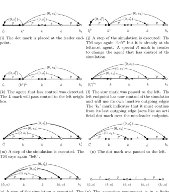
When the control of the simulation reaches a non-leader agent (e.g. from the left leader endpoint side) in order to visit its first edge it places the dot mark to the left leader endpoint and then to the next (on the right) non-leader and so forth. If the dot mark reaches the star-marked agent (in the previous example from the left endpoint side) then it moves the dot to the closer (in the pseudo-path graph) agent that can “see” via an inactive edge towards the right non-leader endpoint. In this way, each agent visits its outgoing edges in a specific sequence (from leader to non-leader when the simulation moves right and the reverse when it moves left) providing theO(n2) space needed for the simulation. See Figure 4 for a graphical example.
However the inactive edges of each agent towards the rest of the population are asymptotically sufficient for the simulation discussed so far.
(a) The agent ink∗controls now the simula-tion.
(b) A step of the simulation is executed on the inactive edge. The TM says “right” so k∗must next run the simulation on the first inactive edge to the right.
(c) Markrtravels to the right until it meets the first agent that has an incoming inactive edge fromk∗.
(d) The mark still travels.
(e) The correct agent was found. The special dot mark will make the simulation run on the next inactive edge.
(f) A step of the simulation is executed. The TM says now “left” so the simulation must next use again the previous inactive edge.
(g) The dot mark is placed on the wrong agent (because we only use for the simulation the inactive outgoing edges ofk∗).
[image:23.595.135.475.168.399.2](h) The error is detected because the interac-tion happened through an active edge. Thel mark continues its travel to the left.
Figure 4: An example of simulating aO(n2)-space deterministic TM. The simulation is
per-formed on the second (state) component of the inactive edges (those whose first component is 0). The bold edge indicates the pair that has just interacted. The black agent is the initiator and the grey the responder. The states of the corresponding agents are updated in each figure according to their previous states and the state of the edge joining them. We only present the effective interactions that take place; it is possible that between two subsequent figures a finite number of ineffective interactions have taken place. Fairness guarantees that an effective interaction that is always possible to occur will eventually occur (continued...).
(i) The dot mark is placed at the leader end-point.
(j) A step of the simulation is executed. The TM says again “left” but it is already at the leftmost agent. A specialRmark is created to change the agent that has control of the simulation.
(k) The agent that has control was detected. TheLmark will pass control to the left neigh-bor.
(l) The star mark was passed to the left. The left endpoint has now control of the simulation and will use its own inactive outgoing edges. The ‘kt’ mark indicates that it must continue
from its last outgoing edge (acts like an arti-ficial dot mark over the non-leader endpoint.
(m) A step of the simulation is executed. The TM says again “left”.
(n) The dot mark was passed to the left.
(o) A step of the simulation is executed. The TM accepts and an accepting component is created in both agents.
[image:24.595.136.473.173.556.2](p) The accepting component is in a finite number of steps (due to fairness) propagated to all agents and the population also accepts.
components, one used to identify them as active/inactive and the other used by the simulation (protocolAfrom Theorem 8).
This time, the reinitialization process attempts to reinitialize not only all agents of a pseudo-path graph but also all of their outgoing edges. We begin by describing the reinitialization process in detail. Whenever the merging process of two pseudo-path graphs comes to an end, resulting in a new pseudo-path graph
L, the leader endpoint ofLgoes to a specialblocked state, let it belb, blockingL
from getting merged with another pseudo-path graph while the reinitialization process is being executed. Keep in mind thatLwill only get ready for merging just after the completion of the reinitialization process. By interacting with its unique right neighbor in statekvia an active edge it propagates the blocked state towards that neighbor updating its state tokb and reinitializing the agent. The
block state propagates in the same way towards the tail non-leader reinitializing and updating all intermediate non-leaders to kb from left to right. Once it
reaches this endpoint, a new special statek0 is generated which traversesL in the inverse direction. Oncek0 reaches the leader endpoint, it disappears and the leader updates its state tol∗.
Now reinitialization of the inactive edges begins. When the leader in l∗
interacts with its unique right neighbor (via the active edge joining them) it updates its neighbor’s state to a special bar state (e.g. ¯k). When the agent with the bar state interacts with its own right neighbor, which is unmarked, the neighbor updates its state to a specialdot state (e.g. ˙k). Now the bars cannot propagate and the only effective interaction is between the star leader and the dot non-leader. This interaction reinitializes the state component of the edge used for the simulation and makes the responder non-leader a bar non-leader. Then the new bar non-leader turns its own right neighbor to a dot non-leader, the second outgoing edge of the leader is reinitialized in this manner, and so on, until the edge joining the star leader (left endpoint) with the dot tail non-leader (right endpoint) is reinitialized. What happens then is that the bars are erased one after the other from right to left and finally the star moves one step to the right. So the first non-leader has now the star and it reinitializes its own inactive outgoing edges from left to right in a similar manner. The process repeats the same steps over and over, until the right endpoint ofLreinitializes all of its outgoing edges. When this happens,Awill execute its simulation on the correct reinitialized states. The above process is clearly executed correctly whenLis spanning (because all outgoing edges have their heads on the pseudo-path graph). When it isn’t, the correctness of the process is captured by the following lemma.
Lemma 3. LetLandL0 be two distinct pseudo-path subgraphs ofG. IfLruns a reinitialization process then it always terminates in a finite number of steps.