Monograph:
Stillwell, J. and Dennett, A. (2008) Internal Migration in Great Britain – A District Level Analysis Using 2001 Census Data. Working Paper. The School of Geography, The University of Leeds
School of Geography Working Paper 08/1
[email protected] https://eprints.whiterose.ac.uk/
Reuse
Unless indicated otherwise, fulltext items are protected by copyright with all rights reserved. The copyright exception in section 29 of the Copyright, Designs and Patents Act 1988 allows the making of a single copy solely for the purpose of non-commercial research or private study within the limits of fair dealing. The publisher or other rights-holder may allow further reproduction and re-use of this version - refer to the White Rose Research Online record for this item. Where records identify the publisher as the copyright holder, users can verify any specific terms of use on the publisher’s website.
Takedown
If you consider content in White Rose Research Online to be in breach of UK law, please notify us by
analysis using 2001 Census data
Adam Dennett and John Stillwell
School of Geography
University of Leeds
LS2 9JT
[email protected]
March 08
Full contact details of the authors are:
School of Geography, University of Leeds, Leeds,
LS2 9JT
Tel: +44 (0 in UK) 113 34 33300 Fax: +44 (0 in UK) 113 34 33308
Adam Dennett
John Stillwell
This paper makes use of the Special Migration Statistics (SMS) from the 2001 Census to explore the magnitude, composition and pattern of population migration within Great Britain. Age and sex differentials are examined through the use of migration schedules, whilst spatial patterns of net migration balances and rates are explored using other graphic and cartographic techniques. Much of this analysis is bound within a district classification framework; the use of which, in conjunction with these techniques, has helped reveal new characteristics and patterns. In
sess population stability for
districts and area classification aggregations thereof within Britain analysis which helped overcome some of the limitations inherent in standard net rate calculations.
Our findings are that at an aggregate level, familiar past trends such as counterurbanisation can still be identified, but by using the Vickers et al. classification, these aggregate migration patterns can been deconstructed, revealing spatially varied trends of both counterurbanisation and urbanisation across Britain. Population stability, defined by turnover and churn analysis, is broadly reduced in urban areas and increased in rural areas, although stability varies greatly across age groups. Following these findings it is useful to conceptualise a two-tier Britain; a rural Britain with a relatively stable population, characterised by some in-migration, and a rural Britain with a far less stable population featuring migrants with characteristics similar to those found in London. Finally we find that the effect of age and sex on the propensity to migrate is key, however these attributes interact with the particular socio-demographic, economic and environmental characteristics of places (as characterised by the Vickers et al.
Table of Contents
Table of Contents ... iv
List of Figures ... v
List of Tables ... vi
1. Introduction ... 1
2. Recent studies of internal migration in the UK ... 2
3. Research framework ... 8
4. Data sources and issues ... 10
5. Aggregate patterns of internal migration ... 23
6. Inflow/outflow by sex ... 28
7. Migration schedules by age and sex ... 28
8. Migration patterns for districts by broad age group ... 36
9. Migration schedules by district classification ... 52
10. P ... 59
11. Discussion of findings and conclusions ... 80
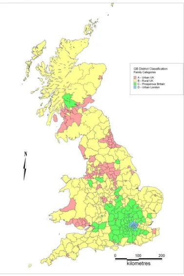
Figure 1. Vickers et al. District Classification: Family categories, Britain ... 14
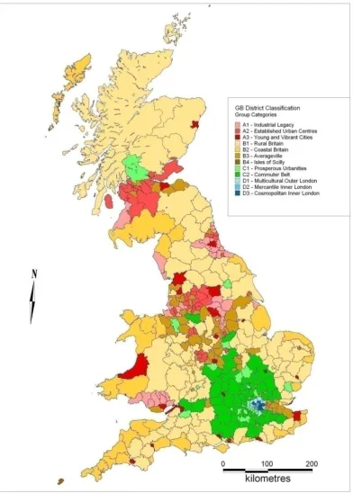
Figure 2. Vickers et al. District Classification: Group categories, Britain ... 15
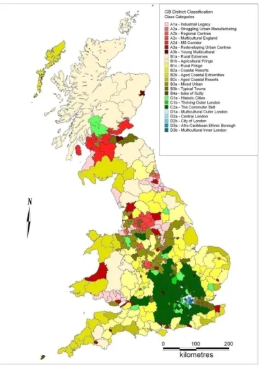
Figure 3. Vickers et al. District Classification: Class categories, Britain ... 16
Figure 4. District level flow matrix including an example hierarchical geo-demographic classification ... 20
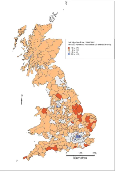
Figure 5. District net migration rates (per 1,000 population) all ages, 2000-01 ... 25
Figure 6. In-migration/out-migration ratios for district types in Britain by sex, 2000-01 ... 27
Figure 7. District level internal migration schedule for Britain, 2000-2001 ... 30
Figure 8. District level internal migration rate schedule for Britain, 2000-2001 ... 30
Figure 9. District level internal migration rate schedule for Britain, 2000-2001, by smallest possible age groups, 0 to 29 years ... 31
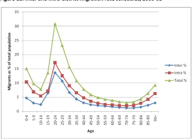
Figure 10. Inter and intra-district migration schedules, 2000-01 ... 34
Figure 11. Inter and intra-district migration rate schedules, 2000-01 ... 34
Figure 12. Inter and intra-district migration schedules by sex, 2000-01 ... 35
Figure 13. Inter and intra-district migration rate schedules by sex, 2000-01... 35
Figure 14. District level migration rates (per 1,000 population) 0-15 age group, 2000-01 ... 39
Figure 15. District level migration rates (per 1,000 population) 16-29 age group, 2000-01 ... 41
Figure 16. District level migration rates (per 1,000 population) 30-44 age group, 2000-01 ... 44
Figure 17. District level migration rates (per 1,000 population) 45-pensionable age group, 2000-01 ... 46
Figure 18. District level migration rates (per 1,000 population) pensionable age and above age group, 2000-01 ... 49
Figure 19. In-migration/Out-migration ratios for district types in Britain by broad age group, 2000-01 ... 51
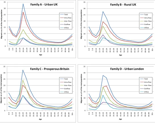
Figure 20. Age-specific migration rate schedules for total inflow, outflow, intra-Family, inter-Family and total flows, for the four Vickers et al. classification district Family categories ... 53
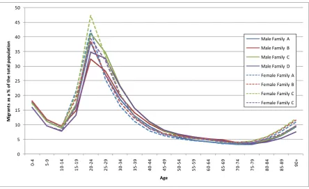
Figure 21. District level migration rate schedule disaggregated by Family category of district and sex for Britain, 2000-01 ... 55
Figure 22. District level migration rate schedules, disaggregated by Group category of district, 2000-01... 57
Figure 23. District level in-migration rate schedule, disaggregated by Group category of district, 2000-01 ... 58
Figure 24. District level out-migration rate schedule, disaggregated by Group category of district, 2000-01 .... 58
Figure 25. Net migration rate against turnover rate for all districts in Britain, 2000-01 ... 62
Figure 26. Net migration rate against churn rate for all districts in Britain, 2000-01 ... 62
Figure 27. Turnover rate against churn rate for all districts in Britain, 2000-01 ... 63
Figure 28. Intra district flow rate against turnover rate for all districts in Britain, 2000-01 ... 63
Figure 29. District population turnover rates (per 1,000 population) total population, 2000-01 ... 71
Figure 30. District population churn rates (per 1,000 population) total population, 2000-01 ... 71
Figure 31. District population turnover rates (per 1,000 population) 0-15 age group, 2000-01 ... 72
Figure 35. District population turnover rates (per 1,000 population) 30-44 age group, 2000-01 ... 74
Figure 36. District population churn rates (per 1,000 population) 30-44 age group, 2000-01 ... 74
Figure 37. District population turnover rates (per 1,000 population) 45 to pensionable age group, 2000-01 . 75 Figure 38. District population churn rates (per 1,000 population) 45 to pensionable age group, 2000-01 ... 75
Figure 39. District population turnover rates (per 1,000 population) pensionable age and above age group, 2000-01 ... 76
Figure 40. District population churn Rates (per 1,000 population) pensionable age and above age group, 2000-01 ... 76
List of Tables
Table 1. Example of the proportions of each ward assigned to each associated district in Northern Ireland ... 12Table 2. Summary of flows for areas at Family, Group and Class level of Vickers et al. Classification ... 24
Table 3. Net migrants and net migration rates by district classification all ages, 2000-01 ... 26
Table 4. Percentage of age group population who are migrants ... 37
Table 5. Net migrants and net migration rates by district classification 0-15 age group, 2000-01 ... 40
Table 6. Net migrants and net migration rates by district classification 16-29 age group, 2000-01 ... 42
Table 7. Net migrants and net migration rates by district classification 30-44 age group, 2000-01 ... 45
Table 8. Net migrants and net migration rates by district classification 45-pensionable age group, 2000-01 . 47 Table 9. Net migrants and net migration rates by district classification pensionable age and above age group, 2000-01 ... 50
Table 10. Summary of the count of districts falling within each net-migration range by broad age group ... 52
Table 11. A comparison of net migration, population turnover and population churn statistics for classifications of district in Britain, 2000-01 ... 65
Table 12. Turnover and churn calculations for Vickers et al. classification families, standardised by age ... 67
1.
Introduction
The importance of studying internal population migration within the UK has long been recognised. Internal migration is a major contributing factor to population change in almost all areas of the country. This involves not only change in the numbers of people (although this is important in itself), but also the change in the composition and structure of local populations which can have implications for issues such as service provision, social cohesion, the physical environment and local economic development. Detailed knowledge of intra-national movements of the population has been important for a long time. Recognising this, various studies have been carried out over the years all of which have enhanced our knowledge and understanding of the trends in internal population movements at a range of spatial scales and over different periods of time.
2.
Recent studies of internal migration in the UK
A number of authors have considered aggregate internal population migration trends in the UK. Stillwell and Boden (1986) used Census and National Health Service Central Register (NHSCR) data to examine aggregate national (British) patterns of migration between the 1961 and 1981 Censuses. They showed that, on a national level, the rate and level of migration increased throughout the 1960s before entering into a noticeable decline during the 1970s from 5.8 million migrants in 1970-71 to 4.7 million in 1980-81. Over the two decades, the majority of migrants were female, although rates were higher for males. Stillwell and Boden acknowledge the limitations of decennial census data, especially where there is a desire to understand inter-censal movements. To address this they use annual movements estimated from the NHS Central Register between 1975 and 1983, focusing specifically on age-related migration schedules. They conclude that whilst a decline in the level of mobility can be seen in the 1970s when compared to the previous decade, the age and sex characteristics of migrants remained relatively stable.
Rees and Stillwell (1987) extend this national aggregate picture of internal migration through examining internal migration in regional and metropolitan/non-metropolitan contexts. Again the principal data sources are the census and NHSCR re-registration data, this time from the mid-1960s to the mid-1980s. The regional pattern over this twenty year period is one of the northern periphery (including Northern Ireland, and Scotland), the Industrial Heartlands (including the North West, Yorkshire and the Humber, the West Midlands) and Greater London all experiencing net out-migration, with the south (including the East Midlands, East Anglia, the East and South West) experiencing net in-migration. This north-south shift has also been identified by authors including Champion (1989b) and Owen and Green (1992). A regional perspective on migration at this time was also taken by Ogilvy (1982) using the NHSCR data. As might be expected, comparable findings were presented, although Ogilvy placed emphasis on the drop in out-migration from the South East during the 1970s rather than the increase in in-migration as the reason for continued net gains.
Whilst these regional patterns add detail to the national scene depicted by Stillwell and Boden (1986), it is recognised by Rees and Stillwell (1987) that the examination of trends at a regional scale can mask important movements between metropolitan and non-metropolitan areas. During this time period, the dominant trend is one of a decentralisation of population, with
metropolitan areas to non- I Britain at this time has been reported elsewhere by Kennett (1980), Champion (1989a, 1994) and Cross (1990).
The loss of population from metropolitan to non-metropolitan areas recognised throughout the 1970s did not abate in the 1980s. Stillwell et al. (1992) note the continuing trend of metropolitan out-migration throughout this decade. In volume terms, the last three years of the 1980s saw counterurbanising moves account for 37% of the total internal migration movements (according to NHSCR patient re-registration data) when compared to north-south moves accounting for only 27% of total internal migration movements. It is further demonstrated that, in the 1980s, the metropolitan areas were only gaining population from the student and immediately post-student quinary age-groups. Whilst an overall trend of counterurbanisation in Britain is identified here, when examined closely, the trend is highly region-specific. It is noted that in the north, whilst there was a net out-migration from metropolitan areas, there was not a noticeable corresponding net in-migration to non-metropolitan areas. The trend in the north of Britain was more likely to be the movement from north to south, than the movement from urban to rural. Certainly whilst this north-south movement pattern is the important trend for most of the 1980s, one significant point of interest occurs at the end of the 1980s. Whereas the net flow had been into the south from the north since the mid 1970s, Stillwell et al. (1992) show that an increase in the movement of migrants northwards had in fact tipped the balance slightly in the favour of a net gain to the north in 1989.
Rees et al. (1996) used data from the 1991 Census to show a continuation of the trend of depopulation from urban areas that had been revealed in previous decades. This applied both to the largest metropolitan areas as well as the smaller cities. It was further shown that resource B windling primary industry (such as mining and
offshore industry) were gaining migrants.
Other trends identified were associated with the predominance of the 1-15 and 30-44 year old age groups in the overall patterns of migrant redistribution, and with lower mobility but clearer patterns of redistribution at retirement and post-retirement ages. There was a noticeable urbanisation of the 16-29 age group, associated with student movements to higher educational institutions which were often found in large urban areas a trend familiar from previous
population from cities, meaning that population was redistributed both down the urban hierarchy from larger to smaller urban centres, and out from urban centres into rural fringes. The latter did not necessarily indicate the return of a desire by people to live rural lifestyles, but rather was the result an expansion of pre-existing urban systems into areas otherwise identified as rural.
Looking into these patterns in more detail it was noted that there appeared to be a propensity within the migrant population to move from higher to lower density areas on the whole; this was coupled with a shift from areas suffering from above average unemployment to areas with below average unemployment. Indeed, all of the findings by Rees et al. echo and bolster the regional level work of Stillwell et al. (1995) for the same period. Subsequent work by Kalogirou (2005) on England and Wales, lends further weight to these findings.
A further overview of internal (and international) migration in this period is provided by Champion et al. (1998). As would be expected, the aggregate patterns recounted are no different from those already covered in this review. Where this latter overview differs is that it brings into focus the issue of scale. Work already mentioned has examined migration at different spatial scales; however, here the effect of scale on results is discussed explicitly. Due to the preponderance of short distance moves over longer distance moves, inter-area flows become more important when the scale of analysis is smaller. In addition, regional level analysis will, for example, emphasise the importance of international migration as the major component of population change, whereas analysis at more disaggregate scales will promote the importance of internal migration.
on employment as an explanatory factor for internal migration), and Cameron et al. (2005) (which turns its attention to housing), each offer persuading evidence of the influence of employment and housing respectively on regional level internal migration.
Thus far we have reviewed work which has drawn on data available before the 2001 Census. Despite internal migration data from the 2001 Census being available since 2003, there has been relatively little work carried out on internal migration patterns in the new millennium.
S ONS F O
publication in which Champion (2005) provides a wide ranging overview of internal migration in the UK, drawing principally (although not exclusively) from the 2001 Census.
Champion indicates that, in 2000-2001, there were around 6.7 million internal migrants nationally, but comments that little difference is evident in the migration propensities of males and females; at least at an aggregate level (propensities vary much more with age). Where age (the other key demographic indicator often mentioned with sex) is concerned, however, the situation is somewhat different. The trend in 2001 (as in previous years) is that young adults have the greatest propensity to migrate. This coincides with the now familiar movement of many in their late teens to university, and then away from these locations as students move on to their first jobs after completing higher education courses. The tendency to migrate reduces with age after young adulthood until around the age of 75. As in previous years, age-specific migration follows a familiar pattern with a reduction in the propensity to migrate from the mid-twenties to the mid-thirties, corresponding with family raising and the desire for settled child rearing. This decline in migration propensity continues until around pensionable age. From here there is a noticeable increase in the rate of migration and this can be attributed to the nd insecurity increases with age. Migration at this age can readily be attributed to moves associated with a greater need for care or to be within proximity of family.
were generally less likely to migrate. The white ethnic group also had marginally lower migration tendencies than non-white groups.
Champion examines some of the sub-national migration patterns that are displayed by the results of the 2001 Census. At the district and ward level, the salient point is that districts and wards with the highest proportions of people living at a different address one year ago tend to be those with highest student populations. Unlike the 1991 Census, when students were recorded at their parental domiciles, the 2001 Census recorded students at their term-time
A
those districts and wards with the lowest proportions of their populations consisting of people who lived at a different address one year previously were frequently located in Northern Ireland. Mapping reveals the relative importance of coastal and rural retirement areas where higher migratory rates are present.
Another key feature of internal migration from the 2001 Census picked out by Champion is the pervasiveness of net urban-rural migration across the whole of the UK not just where London is concerned. Using a classification of districts adapted from work carried out in the early 1980s, he demonstrates that metropolitan areas are continuing to lose migrants to rural areas. The validity of using a classification for areas devised in the 1980s should be questioned to some extent, especially when considering the amount of change that has taken place in the socio-demographic and physical characteristics of many of these areas since then. However, one might suspect that, under scrutiny, these broad patterns are likely to be more-or-less accurate at this aggregate level.
Finally Champion takes a somewhat more detailed look at the geographical variations in the interaction flows of four specific population characteristics: age, student status, ethnic grouping and higher managerial and professional occupations are examined at a regional scale. He concludes that there is a rural/urban association with age, in that younger age groups may be
highest socio-economic groups, with areas to the south-west and east of the country recording the lowest net gains.
3.
Research framework
This paper can be further set within a two component theoretical framework out of which the principal research questions arise. One of the central strands of migration research has always attempted to tackle the external causal influences affecting migration behaviours. This provides
the first component of our framework. S ‘ ‘
1889) where the employment related economic attractions of urban areas were recognised in partnership with the relative dearth of employment opportunities in rural areas, the former resulting in a migration flow from the latter, research on the factors influencing migration behaviour and flows between particular places has been abundant. A variety of empirical analyses including those offered by Fielding (1992), Champion et al. (1998) Cameron et al.
(2005) Norman et al. (2005) and Finney and Simpson (2007), examine the differing effects of the social, economic and environmental characteristics of places on particular migration behaviours. These kind of empirical analyses with observations regarding the influences on migration have served as the foundation for variety of models used both to increase understanding of the processes influencing internal migration and to project migration behaviours into the future; the most ambitious of these probably being the migration model for the UK developed by Champion
et al. for the then Office of the Deputy Prime Minister (ODPM, 2002). All of this work, however,
has helped confirm the idea that migration behaviours are heavily influenced by the particular characteristics of both origins and destinations, and it is partially within this framework that this paper positions itself. A large section of this work will be devoted to answering the question of what particular influence area types, and implicitly the characteristics of these areas, have on the volume and direction of internal migration experienced.
Another key strand of migration research has focused on the attributes of the individual migrant, and how these may affect migration behaviours. Age, sex, ethnicity, socio-economic
e. This
2000-01, and answering the question of what particular age related features of internal migration exist at this time.
4.
Data sources and issues
The data used in this analysis are principally the 2001 Census Special Migration Statistics (SMS). These data are derived from the question pertaining to place of usual residence one year before the Census. More specifically, the data used have been taken from the SMS level 1 tables
L B U
Authorities, Metropolitan and Non-Metropolitan Districts, Scottish Council Areas and other Local Authority Districts) in the UK. Data at this level are likely to be more accurate than the same data at level 2 (ward level) and level 3 (output area level) due to the effect of the small cell adjustment method (SCAM) on values of 1 and 2 in the tables. Essentially, the larger the spatial scale of study, the less likely it is for small values to be recorded and subsequently adjusted by SCAM. Stillwell and Duke-Williams (2007) provide a more detailed explanation of the effects of SCAM.
In addition to the effects of SCAM, whilst ward and output area level data would give a much higher spatial resolution in the analysis, the additional resolution may in fact reduce clarity and make the identification of patterns more problematic when presenting a national overview. The issue of the Modifiable Areal Unit Problem (MAUP) should be acknowledged (Openshaw, 1984). The MAUP highlights the issues of scale and aggregation when presenting results for discrete geographical areas. One way to deal with this problem would be to carry out analysis at a variety of different scales, but this would create an overly extensive analysis that would then also run into problems with small cell adjustment. At this stage the use of rates standardised by populations for discrete geographical units should minimise the problem of the MAUP. It is important, however to acknowledge that the use of districts may affect the outcome of the analysis to some degree.
The analysis of districts will be carried out for Great Britain, rather than the whole UK. Northern Ireland has been omitted from the analysis for a variety of practical reasons. Firstly, there are no interaction data available for Northern Ireland at level 1 (the district scale) for district areas Northern Ireland data at level 1 are only available for Parliamentary Constituencies. Whilst these areas are broadly comparable with districts in terms of size, their geographical boundaries are different, thus causing a set of harmonisation problems.
are available for the whole of the UK. As previously noted, the effect of small cell adjustment at any level below district is especially marked for interaction data due to the higher proportions of small numbers of migrants in each area. Furthermore, output areas and wards are too small to allow the easy identification of national patterns and trends through cartographic techniques. These reasons in themselves should be enough to justify the use of districts for a national study, thereby necessitating the omission of Northern Ireland as data are not available at this level. In addition though, a robust district level classification has been developed by Vickers et al. (2003) which will enable the study of interaction flows both at district level, and at the three subsequent levels of aggregation in the classification. Whilst Northern Ireland features in the classification, Northern Ireland districts rather than parliamentary constituencies are used. Thus, it follows that if the data for Northern Ireland were to be used at all, it would need to be at the district level. A full justification for the use of the Vickers et al. classification in this study is given later on.
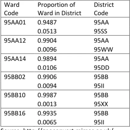
Table 1. Example of the proportions of each ward assigned to each associated district in Northern Ireland
Ward Code
Proportion of Ward in District
District Code
95AA01 0.9487 95AA
0.0513 95SS
95AA12 0.9904 95AA
0.0096 95WW
95AA14 0.9894 95AA
0.0106 95DD
95BB02 0.9906 95BB
0.0094 95II
95BB10 0.9987 95BB
0.0013 95XX
95BB16 0.9935 95BB
0.0065 95II
Source: http://geoconvert.mimas.ac.uk/
There are two issues here. The first issue relates to the geographic location of addresses within the ward. For example, it could be the case that there are no addresses featured in the small proportion of the ward associated with one district. Where this is the case, there would be no need to reallocate a proportion of the data to this district. On the other hand, this very small portion of the ward could contain a considerable proportion of the addresses, requiring the
T
that even if the proportion of addresses allocated from a ward to districts is known (something that is feasible, if not practically possible for large areas through the address counts available in the all fields postcode look-up directory tables), it is almost impossible to allocate appropriately the correct data to the correct addresses especially for a large amount of areas where many calculations would be needed. Furthermore, address counts will include communal establishments (such as student halls of residence, hotels, hospitals and prisons) as well as households which more commonly accommodate smaller numbers of residents, making data allocation even more difficult.
[image:19.595.89.306.110.328.2]wards for Northern Ireland, for both origins and destinations; this would also need to be accompanied by the information for every district in the rest of the UK. This means that for each of the 990 origins (408 districts in England, Wales and Scotland and 582 wards in Northern Ireland) there would also be 990 destinations. This would be a pairwise list of some 980,100 rows of data if one were downloading a list of every variable by every origin/destination pair. Alternatively it would be a 990 by 990 matrix for each variable selected. Whatever the format used for downloading, the flow data for every Northern Ireland ward would need to be weighted appropriately and then assigned to a new district. This would be a considerable task!
What use can classifications be in the study of population flows in Britain? Classifications are effective ways of summarising areas in terms of their key characteristics and, as such, provide a useful backdrop upon which to project other information, such as population migration flows. It is then possible to see if areas with similar socio-demographic characteristics have similar migration characteristics. The Vickers et al. classification does not incorporate data on migration and so provides a framework for the migration analysis which is independent of the influence of migration variables.
Studies in the past by authors such as Champion (2006, 1989a) and Fielding (1992) have sought
L UK
Studying migration in the context of this classification allows for the identification of migration trends and patterns in relation to these traditional binaries, but in addition, the sub-classifications (Families, Groups, Classes) mean that movements can be further broken down into migration into or out of types of rural and urban area, or very specific parts of London. This is of significant benefit as binary definitions may be masking certain types of flow. For example, a general pattern of counterurbanisation in Britain could be obscuring patterns of urbanisation in relation to some key urban areas. By using the Vickers et al. classification, there is scope to study migration at a more detailed level.
It should be acknowledged that the Office for National Statistics (ONS) has also created an area classification for local authorities (districts) (http://www.statistics.gov.uk/about/methodology _by_theme/area_classification/la/default.asp). So why has the official classification used by the ONS has not been used in this analysis? The methodology outlining the selection of variables and clustering techniques used in the Vickers et al. classification is more comprehensive, robust and transparent than the methodology behind the ONS classification. As such, one can be more assured that the ascribed characteristics in the Vickers et al. classification accurately reflect the character of the districts classified in that way.
It may be that the selection of variables and clustering techniques in the ONS classification of
V n. However, the
accompanying methodology published does not lead one to believe this. For example, the stated method of variable selection for the ONS classification was that they were selected
series of team meetings using a rigorous and logical approach, designed to gain an efficient
C (http://www.statistics.gov.uk/ about/methodology_by
H entirely sure of exactly how rigorous and logical the approach actually was? Without full explanation, one is not entirely sure that the decision did not come out of a subjective
ONS
In contrast to this rather unclear justification in the ONS methodology, Vickers et al. (2003) describe in detail the methodology that was used in the selection of variables to build their classification. A list of 129 variables was assembled from the 2001 Census, using variables from previous classifications as a baseline, and adding new variables that appeared for the first time in 2001. These variables were then assessed in terms of the information they could provide about an area (for example, if every area in a country contained exactly the same number and proportion of males and females, a sex variable would probably not tell you an awful lot about that area. If, however, these numbers and proportions were wildly different for every area in a country, then a sex variable would probably tell you quite a lot). In order to assess these variables in terms of the information they contained, a suite of methods were employed by Vickers et al. Firstly, principal components analysis was used to assess the relative importance of the different components of a variable (for example, different age groups within an age variable). Secondly, highly correlated variables were discarded. Thirdly, the variance of the variables across the study area was examined, with the higher variance variables being preferred (Vickers et al. 2003).
After the implementation of this rigorous selection methodology, 56 variables were selected in the Vickers et al. classification in comparison to the 42 variables used in the ONS classification. Whilst one cannot be completely certain that these 56 variables help constitute a more accurate classification of districts in the UK, the methodology behind selection is fully explained and is logical, backed up with statistical evidence. In the absence of a comparatively detailed ONS methodology, justification for choosing the ONS classification (despite its assumed superiority as
V et al. classification cannot be made.
Finally, it should be noted that there are distinct similarities between the two classifications, meaning that the choice of one over the other is unlikely to yield strikingly different results in an analysis. Whilst ONS does not clearly outline the method for selecting variables, it does describe
I W
in combination with the K-means method was used to define the clusters in the classification.
Furthermore, upon examination of the final variables used in each classification, there are a number of similarities, with similar demographic, household, health, housing, socioeconomic and employment variables being used in both classifications.
District 1 District 2 District 3 District 4 District 5 District 6 District 7 District 8 District 9 District 10 District 11 District 12 District 13 District 14 District 15 District 16 D is tr ic t 1
154 0 9 3 9 15 44 6 16 3 17 70 25 16 3 3 239
4 4 2 D is tr ic t 2
0 6844 24 29 52 18 29 15 28 42 63 59 3 31 21 1385
1 7 9 9 3 4 4 8 D is tr ic t 3
19 46 15168 33 1161 88 1174 93 278 1380 120 251 221 1178 890 37
6 9 6 9 1 5 2 3 5 D is tr ic t 4
0 38 25 8524 21 657 39 44 28 16 1217 44 8 29 6 81
2 2 5 3 5 5 9 3 D is tr ic t 5
11 80 1383 66 13198 75 837 150 1269 217 119 266 379 408 2252 25
7 5 3 7 1 3 7 1 9 D is tr ic t 6
12 44 62 560 53 13123 84 959 59 66 438 40 41 48 47 25
2 5 3 8 5 7 5 6 D is tr ic t 7
65 45 1909 52 1174 77 10966 90 296 279 185 689 464 1662 206 34
7 2 2 7 1 2 2 6 6 D is tr ic t 8
0 32 128 108 73 1134 131 17798 88 105 143 60 79 61 56 18
2 2 1 6 4 3 1 4 D is tr ic t 9
7 25 302 23 1005 79 285 111 15068 137 88 253 830 206 861 13
4 2 2 5 8 8 8 1 D is tr ic t 1 0
3 97 1269 76 158 61 242 82 114 13850 78 280 65 1347 100 58
4 0 3 0 1 0 3 8 3 D is tr ic t 1 1
3 68 102 2168 58 709 130 75 77 61 11102 104 60 86 49 68
3 8 1 8 6 7 6 2 D is tr ic t 1 2
31 352 325 53 243 72 493 110 161 693 125 9658 124 1405 48 137
4 3 7 2 7 8 3 5 D is tr ic t 1 3
31 37 222 32 505 93 444 133 1529 62 112 211 8444 205 133 18
3 7 6 7 6 3 8 9 D is tr ic t 1 4
12 97 1793 52 377 70 893 144 254 3166 162 1040 215 10795 81 44
8 4 0 0 1 5 2 0 7 D is tr ic t 1 5
9 18 662 9 1281 42 204 60 430 86 46 69 90 97 8453 6
3 1 0 9 7 8 8 3 D is tr ic t 1 6
0 670 51 76 12 28 10 26 29 40 31 27 18 28 21 8231
1 0 6 7 3 0 1 9
203 1649 8266 3340 6182 3218 5039 2098 4656 6353 2944 3463 2622 6807 4774 1952
154 6844 15168 8524 13198 13123 10966 17798 15068 13850 11102 9658 8444 10795 8453 8231
Class Intra Group Intra Family Intra District Inflow Class Inflow Group Inflow Family Inflow District Intra 30916 101479 16910 17693
6998 23750 26449 28985 29169 20989 19659 16711
6178 9009 6699
13232 11700 15245 15199
1852 11548 9272 6916 10758
234942
Total Migrants Destination j O ri g in i G ro u p A2 Cla
ss A 2 a C la ss A 2 b Fa m il y B G ro u p B
1 Cla
ss B 1 a C la ss B 1 b G ro u p B 2
Group A1 Group A2 Group B1 Group B2
Family A Family B
Class A2b Class B1a Class B1b Class B2a Class B2b Class A1a Class A1b Class A2a
Fa m il y A G ro u p A
1 Cla
ss A 1 a C la ss A 1 b C la ss B 2 a C la ss B 2 b 7 9 6 1 1 1 7 4 7 4 1 4 9 1 5 3 8 7 1 4 2 7 4 1 4 6 8 1 1 1 0 3 4
59922 51849 36879
98860 D is tr ic t O u tf lo w C las s O u tf lo w G ro u p O u tf lo w F a m il y O u tf lo w 2 0 3 8 9 1 6 4 9 9 4 7 9 2 2 2 8 0 0 4 1 7 6 9 3 1 6 9 1 0 3 8 9 0 2 0 7 1 2 1 9 2 1 9 1 6 1 3 8 1 8 7 6 2 1 4 1 3 9 2 0 7 5 6 1 0 8 4 8 2 4 2 6 6 2 6 3 8 1 2 9 5 1 9 3 0 5 8 6 3 4 6 0 3 3 4 6 0 3 D is tr ic t In te r C las s In te r G ro u p In te r F a m il y In te r
Figure 4 helps to understand the problem of calculating inflows, outflows, intra-zonal and inter-zonal flows for the various zones within a geodemographic classification hierarchy using an example system of two Families of district (A and B), each containing two Groups (A1, A2, B1, B2) which in turn contain two Classes (A1a, A1b, A2a, A2b, B1a, B1b, B2a, B2b). The numbers in the cells within the matrix represent the flows between the smallest or primary geographical areas in this case districts. Each district in the matrix can be further identified as part of the area classification at each of three levels. For example, District 1 is part of Class A1a, Group A1 and Family A. Analysing the flows at the primary geography is straightforward, however, calculating the flows for the other levels in the hierarchy is not just a case of summing the primary geography marginal values for each higher level in the hierarchy. This would result in under-counting for intra-zonal flows, over-counting for inflows and outflows and some double counting for inter-zonal flows. The problem is that flows intra-area flows at one level (e.g. district) may become inter-area flows at another level (e.g. Family).
To explain this problem in a little more detail, take the example of districts 3 and 4, which are part of Class A1b. The intra-district flow of districts 3 and 4 are 15,168 and 8,524 people respectively. Summing these two flows to calculate the intra-zonal flow for Class A1b (which would result in a figure of 23,692) would be incorrect as at the Class level, flows between districts 3 and 4 now count as intra-Class flows. Therefore, as highlighted by the blue square, these flows (of 25 and 33) need to be included in the calculation. The true intra-Class flow would be 23,750 individuals. Taking the inflows and outflows, the same theory applies. Just summing the district level inflows and outflows for districts 3 and 4 to create a Class level inflow and outflow, would include these cells of 25 and 33 consequently over-counting the flows. This problem is compounded if the inflows and outflows are combined to calculate an inter-zonal flow. Doing this would result in the double counting of the flows of 25 and 33.
As Figure 4 shows, this problem increases as one moves up the classification hierarchy. The green square (which highlights the Family B flows), reveals that if just the sum of the intra-district flows within Family B (intra-districts 9 to 16) were taken as the intra-Family B count, this would be a massive under-count. The corresponding inter-Family B flows would be hugely over-inflated due to double counting.
of the primary geography. This is fine if the primary geography remains the only level of analysis. Problems arise when the marginal totals might be summed to different levels in the geodemographic classification. Under counting and double counting will happen, adversely affecting the results produced.
This issue is important when we come to compute rates of migration. In this paper, we focus on the two key demographic characteristics, age and sex; for which the migration data comes from SMS level 1, Table MG101. Populations at risk (PAR) for this table have been obtained from Standard Table ST001. It is common practice when studying patterns of migration to calculate standardised rates of movement, as these rates give a measure of migration that is independent of the population size in any given area. Given the previous discussion, the generic net migration rate calculation for any area in the hierarchy can be written as follows:
= 1000
where:
= the net migration rate per 1,000 population in area i = the in-migration to area i
= the out-migration from area i = end of period population of area i
and the age-sex specific calculation is:
= 1000
where:
= net migration rate per 1,000 population for those in age group a and sex s for area i
= in-migrants in age group a and sex s to area i = out-migrants in age group a and sex s from area i
= end of period population in age group a and sex s of area i
5.
Aggregate patterns of internal migration
In this section, the spatial patterns of internal migration for the year preceding the 2001 Census, for different age-sex groups, will be examined. A summary of all flows at each level of the Vickers et al. classification is given in Table 2. It can be seen from Figure 5 that patterns of net gain and loss for migrants of all ages tend to be associated with areas generally recognisable as rural and urban respectively. The majority of Greater London and its surrounding districts, (including those stretching out along the M4) is experiencing net out-migration. Other areas, including Birmingham, Liverpool, Manchester and their surrounding areas, the North East and Glasgow are all experiencing net out-migration. In contrast, the areas covering large parts of East Anglia, the South West, Wales, the Midlands, the North and Scotland are all experiencing net in-migration.
Table 3 provides a summary of the net balances displayed on the map using the Families, Groups and Classes from the original Vickers et al. classification. This explains the continued use
UK B N
between the summed net balances at each level indicating that the balances at Group and Cluster level refer to flows between districts in different Families. The balances in each column of the Net Migrants section of the table therefore sum to zero. The patterns revealed on the map are summarised at the most aggregate Family level with Urban UK and Urban London exhibiting net out-migration and out-migration rates, and Rural UK exhibiting net in-migration. Of the four Families, Rural UK gains the largest number of net migrants; however, a with a larger population at risk, its net in-migration rate of 2.7 people per 1,000 population is considerably lower than the net out-migration rate of 8.5 people per 1,000 population for London.
overall net out-migration. A similar example can be found within the Urban London Family where the City of London is the only Class within the family to be experiencing net in-migration (albeit very small) all other areas are experiencing net out-migration.
Table 2. Summary of flows for areas at Family, Group and Class level of Vickers et al. Classification
Inflow Outflow Intra flow Inter flow Total flow
A: Urban UK 684527 689369 1567495 1373896 2941391
B: Rural UK 885735 827788 1256411 1713523 2969934
C: Prosperous Britain 509954 514937 496172 1024891 1521063
D: Urban London 366769 414891 284323 781660 1065983
A1: Industrial Legacy 133502 138765 369465 272267 641732
A2: Established Urban Centres 304942 321771 730421 626713 1357134
A3: Young and Vibrant Cities 246083 228833 467609 474916 942525
B1: Rural Britain 398253 367600 480035 765853 1245888
B2: Coastal Britain 188565 159269 300907 347834 648741
B3: Averageville 298754 300794 475328 599548 1074876
B4: Isles of Scilly 163 125 141 288 429
C1: Prosperous Urbanities 181474 179630 196202 361104 557306
C2: Commuter Belt 328480 335307 299970 663787 963757
D1: Multicultural Outer London 130264 151211 130521 281475 411996
D2: Mercantile Inner London 107842 119547 60082 227389 287471
D3: Cosmopolitan Inner London 128663 144133 93720 272796 366516
A1a: Industrial Legacy 133502 138765 369465 272267 641732
A2a: Struggling Urban Legacy 86135 94427 201591 180562 382153
A2b: Regional Centres 80539 77344 143639 157883 301522
A2c: Multicultural England 97511 108775 269649 206286 475935
A2d: M8 Corridor 40757 41225 115542 81982 197524
A3a: Redeveloping Urban Centres 179846 164451 354426 344297 698723
A3b: Young Multicultural 66237 64382 113183 130619 243802
B1a: Rural Extremes 60530 59463 102258 119993 222251
B1b: Agricultural Fringe 156581 141819 192793 298400 491193
B1c: Rural Fringe 181142 166318 184984 347460 532444
B2a: Coastal Resorts 46205 38974 74884 85179 160063
B2b: Aged Coastal Extremities 104609 90622 183149 195231 378380
B2c: Aged Coastal Resorts 37751 29673 42874 67424 110298
B3a: Mixed Urban 184092 186403 282967 370495 653462
B3b: Typical Towns 114662 114391 192361 229053 421414
B4a: Isles of Scilly 163 125 141 288 429
C1a: Historic Cities 90420 84814 108962 175234 284196
C1b: Thriving Outer London 91054 94816 87240 185870 273110
C2a: The Commuter Belt 328480 335307 299970 663787 963757
D1a: Multicultural Outer London 130264 151211 130521 281475 411996
D2a: Central London 106827 118552 59928 225379 285307
D2b: City of London 1015 995 154 2010 2164
D3a: Afro-Caribbean Ethnic Borough 87837 95001 57682 182838 240520
D3b: Multicultural Inner London 40826 49132 36038 89958 125996
Legend:
Inflow = Inflow to Family, Group or Class from all other Families,
Groups or Classes. *Not sum of
inflows for districts within
Families, Groups and Classes.*
Outflow = Outflow from Family, Group or Class to all other
Families, Groups or Classes.
*Not sum of outflows for districts within Families, Groups
and Classes.*
Intra flow = Flows within individual Families, Groups or
Classes. *Not sum of flows
within districts for each Family,
Group or Class.*
Inter flow = Sum of inflow and outflow for each Family, Group
or Class.
Total flow = Sum of intra and inter flows for each Family,
A further graphical representation of these patterns can be seen in Figure 6 which graphs the in-migration/out-migration ratios by sex for each Family, Group and Class of district in Britain.
Figure 6. In-migration/out-migration ratios for district types in Britain by sex, 2000-01
In much the same way that the areal aggregations discussed above can mask migration patterns, so too can the aggregate nature of the variables. Whilst there are any number of individual attributes exhibited by a migrant, historically age and sex have provided some of the more interesting insights into migrant behaviour.
0.6 0.7 0.8 0.9 1 1.1 1.2 1.3 1.4 A: Urban UK
A1(a): Industrial Legacy A2: Established Urban Centres A2a: Struggling Urban Manufacturing A2b: Regional Centres A2c: Multicultural England A2d: M8 Corridor A3: Young and Vibrant Cities A3a: Redeveloping Urban Centres A3b: Young Multicultural B: Rural UK B1: Rural Britain B1a: Rural Extremes B1b: Agricultural Fringe B1c: Rural Fringe B2: Coastal Britain B2a: Coastal Resorts B2b: Aged Coastal Extremities B2c: Aged Coastal Resorts B3: Averageville B3a: Mixed Urban B3b: Typical Towns B4(a): Isles of Scilly C: Prosperous Britain C1: Prosperous Urbanities C1a: Historic Cities C1b: Thriving Outer London C2(a): Commuter Belt D: Urban London D1(a): Multicultural Outer London D2: Mercantile Inner London D2a: Central London D2b: City of London D3: Cosmopolitan Inner London D3a: Afro-Caribbean Ethnic Borough D3b: Multicultural Inner London
Inflow/outflow ratio
6.
Inflow/outflow by sex
One may not necessarily expect to find many differences in the migration propensities of males and females in Britain. Certainly, by ignoring the effect of age, this hypothesis could be confirmed: Figure 6 shows that, in most cases, the inflow/outflow ratios for males and females in Families, Groups and Classes of district are very similar; the only real exception to the rule being the City of London where the ratio for males is significantly positive compared to females where it is significantly negative. However, as with many other statistics for this area, the total numbers of migrants to and from the City of London (as with the Isles of Scilly) are extremely low.
Other areas where differences in inflow/outflow ratios between males and females are clearly apparent are in Averageville (more specifically the Typical Towns settlements in Averageville) and the M8 corridor, where males have a marginally negative balance and females have a marginally positive balance. The ratios in all of these cases, however, are very close to 1, and so should perhaps be viewed less significantly than larger differences where the direction of movement is the same.
7.
Migration schedules by age and sex
To fully appreciate differences in internal migratory behaviour between males and females, however, it is important to examine in detail how differences in migration propensity fluctuate with age. In addition, it will also be helpful to look at how sex differences in migratory behaviour change with the distance of migration. Whilst precise distances of migration movements cannot be accurately measured, the proxy of inter-zone and intra-zone flows is a useful substitute. Of course the levels of inter/intra-zone movements will depend completely on the scale of analysis, with the majority of flows for small areas such as output areas being inter-zonal and the majority of flows for large areas such as regions being intra-zonal (for a more detail discussion on the issues of scale, see Gober-Meyers (1978)). Where the scale of analysis remains constant, however, this should not be an issue. This next section will look at the age-specific migration propensity schedules for districts in Britain and will do so for both inter and intra-zonal flows.
migration schedules is a familiar one (Rogers and Castro, 1981) but there are subtle differences between the schedules for males and females. In order to standardise the data, five year age groups have been used across the schedules up to age 89 with a final 90+ category. It was not possible to obtain data for single year age groups. Where quinary age groups might be obscuring interesting features of the data (such as at the lower end of the age scale), reference will also be made to Figure 9 which features sex-specific rates of migration for the original age groups available from the 2001 SMS (which vary in size from single year of age to five year groups).
Figure 7. District level internal migration schedule for Britain, 2000-2001
Figure 8. District level internal migration rate schedule for Britain, 2000-2001
0 200000 400000 600000 800000 1000000 1200000 0
-4 5-9
1 0 -1 4 1 5 -1 9 2 0 -2 4 2 5 -2 9 3 0 -3 4 3 5 -3 9 4 0 -4 4 4 5 -4 9 5 0 -5 4 5 5 -5 9 6 0 -6 4 6 5 -6 9 7 0 -7 4 7 5 -7 9 8 0 -8 4 8 5 -8 9 9 0 + Mi g ra n ts Age Total Male Female 0 5 10 15 20 25 30 35 0
-4 5-9
At the 15-19 age group, there is a sharp change in this downward trend and a divergence between males and females coinciding with the change in the dependency status of children and the move out of the family home, either to college or university or to a first job. The details of this change are examined in more detail in Figure 9. Here it is possible to see that the downward trend continues until age 15 before rising slightly at 16-17 (corresponding to a first wave of school leavers) and then more rapidly at 18-19. The divergence in the propensities of males and females to migrate at the 15-19 stage is marked. Almost 54,000 more females than males are migrating in this age group. This is even more significant when one realises that there are in fact around 75,000 more males in this group of the population. This difference is confirmed when examination of the rates shows that this equates to 15.4% of females compared to only 11.8% of males.
Figure 9. District level internal migration rate schedule for Britain, 2000-2001, by smallest possible age groups, 0 to 29 years
The gap in the propensities of males and females to migrate is maintained for the next age group. Again, females of this age are considerably more likely than males to be migrants, with over 85,000 more females than males migrating a difference in the proportions of migrants of around 4.7%. As mentioned previously however, the broad categories of 15-19 and 20-24 mask
0 5 10 15 20 25 30 35
0 1-2 3-4 5-9 10-11 12-14 15 16-17 18-19 20-24 25-29
M
ig
ra
ti
o
n
a
s
a
%
o
f
th
e
t
o
ta
l
p
o
p
u
la
ti
o
n
Age
some of the finer nuances of age and sex-specific migration patterns. Figure 9 shows that a gap of 4.7% is eclipsed by a gap of 7.4% in the 18-19 age group.
The rates and numbers of migrants decrease at a steady and relatively sharp rate from a peak of migration (both in terms of proportions and total numbers) in the 20-24 age group, until around the 40-44 age group. From this peak, however, where females comprise the largest proportions and numbers of migrants, males take over as being more likely to be involved in migration. In age groups 25-44, around 1-2% more males than females are involved in internal migration.
From age group 45-49 until the age group 70-74, the numbers and rates of migration for males and females become more equivalent, with only negligible differences between both measures. For both sexes the numbers of migrants and rates of migration continue to decrease until 70-74, but the rate of decline is considerably lower than it has been between earlier age groups.
From age group 70-74 upwards, there are further changes in the migration schedule. Migrants as a percentage of the total population begin to increase from this age group, with the proportion of migrants continuing to increase until the last (90+) age group in the schedule. Females again overtake males as the group with the highest proportion of the total population comprising of migrants in this old age range. This gap continues to widen as age increases. In terms of actual migrant numbers, from the 70-74 age group onwards, there is a continued decrease, as might be expected, with the total populations within the progressively older age groups decreasing. The rate of decrease is much lower for females, however, with a drop of only around 12,000 migrants from 70-74 to 90+ for females, compared to around 24,000 for males.
Taking the migration propensities at all ages into consideration, it has been shown that the age range where the greatest differences, and therefore most interest occurs, is between 18 and 24. The evidence points towards a greater propensity for females than males to migrate in their late teens and early twenties, so one may ask why this is the case. Some explanation is offered by Faggian et al. (2007), whose work using data from the Higher Education Statistics Agency (HESA)
may give some clues. These data revel that for all first year students under 21 years of age in UK Higher Education institutions, there were 18,685 more females than males; this certainly accounts for at least part of this phenomenon. Whilst being a student does not necessarily automatically mean that an individual is also going to be a migrant, with a large proportion of students leaving the family home to go and study, it will increase the likelihood of this being the case.
Other possible explanations for the higher intensities of migration among women in this age group might be associated with migration flows involving communal establishments as origins and/or destinations, including prisons, since flows between communal establishments as well as between households are included in the 2001 data. However, data from the Home Office (2003) for 2001 reveals that the migration of female prisoners is relatively insignificant: there were only 810 females living in prisons compared with 15,152 males aged between 18 and 24.
One final possible explanation for the differences between male and female migration propensities at these ages could be to do with the average age differentials within male/female couples. It may well be that many moves are by individuals who are part of a couple, and that in many cases the female member of the couple is younger than the male, thus accounting for some of the difference at each age group.
Figure 10. Inter and intra-district migration schedules, 2000-01
Figure 11. Inter and intra-district migration rate schedules, 2000-01
Disaggregation of these age-specific migration schedules by both sex and intra/inter-zonal flows is shown in Figure 12 and Figure 13. One of the interesting points of note here is that whilst intra-district flows almost always account for more movements than inter-district flows, there is one exception. In the 15-19 age group, male inter-district migrations are greater than male intra-district migrations, perhaps suggesting that, whilst males may be more reluctant than
females to migrate in this age group, when they do migrate there is a desire to move further away from the parental domicile.
Figure 12. Inter and intra-district migration schedules by sex, 2000-01
8.
Migration patterns for districts by broad age group
The preceding figures and discussion reveal in some detail the proportion of the total population of each defined age group that were internal migrants in Britain, in the year prior to the 2001 Census. In this section, the spatial patterns of migration are investigated.
In the case of the migration schedules for the whole of Britain, five year age groups have been used. However, for much of the remaining analysis in this paper the following age groups are used: 0-15, 16-29, 30-44, 45-pensionable age (pensionable age in this case defined as 65 for males and 60 for females) and pensionable age and above. These groups were chosen as they represent groupings of around 15 years, making it possible to draw comparison with the relative numbers of migrants present in each group. These bands also represent recognisable stages in the life course (with one notable exception) ages 0-15 are the dependent child years; ages 30-44 are the family rearing years; ages 45-pensionable age are the years after the children have left home; and pensionable age and above are the retirement years. The one exception is the 16-29 age group. It could be argued that there are a number of key life stages within this age group: leaving home to study or take a first job; graduating and moving to a first job; moving through the early stages of a career; starting a young family. By choosing a single 15 year grouping for this period (despite its usefulness for comparing with other 15 year groupings), some of the most interesting migration peaks, such as those present for the 18-19 age group, will be obscured. Nevertheless, the age-specific migration schedules in Figure 7-Figure 9 reveal that throughout this 15 year age group migration is consistently high, and so despite some smoothing of the peaks, it is still useful to look at this group as a single entity. By way of compromise, the 16-29 age groups will be disaggregated further where appropriate in this analysis and smaller age groups within this larger group will be looked at separately.
Table 4. Percentage of age group population who are migrants
Age group %
0-15 10.46
16-29 23.65
30-44 11.50
45-PA 4.89
PA+ 3.88
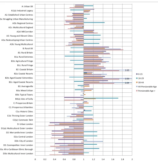
The flows for 0-15 and 30-44 year olds are broadly comparable to the 10.7% observed in the total population, where as the flows for the two oldest age groups (45-pensionable age and pensionable age and above) are considerably lower than the average. Again, the low proportions of migrants in these two groups is not something that should cause surprise. Figure 14 to Figure 18 and Table 5 to Table 9 summarise these patterns for the five different age groups.
Beginning with the youngest age group, 0-15 year olds, there is a clear pattern of net out-migration from urban areas London especially (Figure 14 and Table 5). In the year preceding 2001, Urban London lost almost 23,000 individuals aged 0-15. This was a rate of over 20 people per 1,000 of the 0-15 year old population. This net out-migration from London also included a movement from the area identified as Thriving Outer London, part of Prosperous Britain. In all but the Industrial Legacy and M8 Corridor areas of Urban UK, there was also net out-migration of this age group. Net in-migration of this age group can be found across most of Rural UK and Prosperous Britain, with the highest rates found in the south west of Britain, and outside of the London Commuter Belt area. Paradoxically the highest rates of gain are to be found in the Aged Coastal Resorts.
Figure 16 and Table 7 reveal the patterns of migration for the 30-44 age group. Unsurprisingly this pattern is very similar to that of the 0-15 group, principally because the majority of 0-15 year old migrants will be migrating with parents who are very likely to fall into the 30-44 age category. As with the 0-15 age group, net out-migration is experienced from virtually all Urban UK (except Industrial Legacy areas), and net in-migration can be observed in all areas defined as Rural UK. Significantly there is also net in-migration to areas defined as Commuter Belt, as individuals no-doubt wishing to keep city jobs move out to areas perceived more appropriate for raising their families.
The final age group includes those of pensionable age and above (Figure 18 and Table 9). Essentially the overall migration patterns of this group are very similar to that of the 45 to pensionable age group. These are characterised by net out-migration from Urban London and other built up areas in Urban UK and Prosperous UK, and net in-migration to Rural UK, especially the Coastal Resort areas. Indeed it is noticeable that the only areas of relatively high in-migration for this age group are districts along the south coast, Norfolk and Lincolnshire (Figure 18). One other noticeable pattern is that whilst there is still an overall net out-migration from Commuter Belt areas, this is lower (1.4 people per 1,000 population) than the rate for the preceding age group. Careful examination of the map in Figure 18 reveals further that for a number of Commuter Belt districts in the Home Counties the rate of migration has switched from negative in the 44 to pensionable age group, to positive in the pensionable age and above group.
2.05
2.03 2.04
0 0.2 0.4 0.6 0.8 1 1.2 1.4 1.6 1.8 2
A: Urban UK A1(a): Industrial Legacy
A2: Established Urban Centres A2a: Struggling Urban Manufacturing
A2b: Regional Centres A2c: Multicultural England A2d: M8 Corridor
A3: Young and Vibrant Cities A3a: Redeveloping Urban Centres
A3b: Young Multicultural B: Rural UK B1: Rural Britain
B1a: Rural Extremes B1b: Agricultural Fringe
B1c: Rural Fringe B2: Coastal Britain B2a: Coastal Resorts
B2b: Aged Coastal Extremities B2c: Aged Coastal Resorts B3: Averageville
B3a: Mixed Urban B3b: Typical Towns
B4(a): Isles of Scilly C: Prosperous Britain C1: Prosperous Urbanities
C1a: Historic Cities C1b: Thriving Outer London
C2(a): Commuter Belt D: Urban London D1(a): Multicultural Outer London
D2: Mercantile Inner London D2a: Central London
D2b: City of London D3: Cosmopolitan Inner London D3a: Afro-Caribbean Ethnic Borough
D3b: Multicultural Inner London
0-15 16-29 30-44
44-Pensionable Age
Pensionable Age + Figure 19. In-migration/Out-migration ratios for district types in Britain by broad age group,
[image:58.595.36.572.120.673.2]