The use of heuristic optimization algorithms to
facilitate maximum simulated likelihood estimation
of random parameter logit models
Arne Risa Hole
Hong Il Yoo
ISSN 1749-8368
The use of heuristic optimization algorithms to
facilitate maximum simulated likelihood estimation
of random parameter logit models
Arne Risa Hole
†and Hong Il Yoo
‡†Department of Economics, University of Sheffield
‡
Durham University Business School, Durham University
December, 2014
Abstract
The maximum simulated likelihood estimation of random parameter logit models is now commonplace in various areas of economics. Since these models have non-concave simulated likelihood functions with potentially many optima, the selection of “good” starting values is crucial for avoiding a false solution at an inferior optimum. But little guidance exists on how to obtain “good” starting values. We advance an estimation strategy which makes joint use of heuristic global search routines and conventional gradient-based algorithms. The central idea is to use heuristic routines to locate a starting point which is likely to be close to the global maximum, and then to use gradient-based algorithms to refine this point further to a local maximum which stands a good chance of being the global maximum. In the context of a random parameter logit model featuring both scale and coefficient heterogeneity (GMNL), we apply this strat-egy as well as the conventional stratstrat-egy of starting from estimated special cases of the final model. The results from several empirical datasets suggest that the heuristically assisted strategy is often capable of finding a solution which is better than the best that we have found using the conventional strategy. The results also suggest, however, that the configuration of the heuristic routines that leads to the best solution is likely to vary somewhat from application to application.
Keywords: mixed logit, generalized multinomial logit, differential evolution, particle swarm optimization
1
Introduction
With an increase in desktop computing power, the estimation of the random
param-eter logit model (RPL) has become increasingly common in empirical applications.
Also known as mixed logit, RPL provides a flexible framework for modeling
dis-crete choice data. RPL can approximate any random utility maximization model
arbitrarily well subject to specifying a suitable joint distribution of parameters
(Mc-Fadden and Train, 2000), and readily incorporate preference heterogeneity between different individuals alongside panel correlation across observations on the same
in-dividual (Revelt and Train, 1998). These features make RPL especially attractive
when research questions entail the structural analysis of individual preferences from
a microeconomic perspective. Related applications can be found in various areas
in-cluding environmental economics (Layton and Brown, 2000), labor economics (van
Soest et al., 2002), transportation economics (Small et al., 2005), international
eco-nomics (Basile et al., 2008), and health ecoeco-nomics (Sivey et al., 2012).
While RPL is specified by augmenting the parameters of the multinomial logit
model (MNL) with random heterogeneity, RPL poses a number of estimation issues which MNL does not. Perhaps the best known one is that in most applications, the
RPL likelihood is a multidimensional integral which has no closed-form expression and
needs to be numerically approximated by using simulation. This issue has motivated
several studies to explore how best to obtain a more accurate approximation from
a given number of draws from the joint distribution of random parameters (Train,
2009, pp.205-236), and their findings have popularized the use of Halton sequences to
generate draws. While progress has also been made on developing estimation methods
which are more computationally attractive than the classical method of maximum
simulated likelihood (MSL) in certain aspects (Huber and Train, 2001; Harding and
Hausman, 2007; Train, 2008), MSL still remains the most commonly used method as it can be readily applied in conjunction with almost any joint distribution of random
parameters.
This paper proposes an estimation strategy to address another well-known
estima-tion issue, on which limited practical guidance exists. Specifically, in contrast to its
MNL counterpart, the RPL likelihood is not globally concave and may feature several
local maxima. As in other similar contexts of non-linear estimation, the selection of
inferences based on the estimates associated with an inferior local maximum. In the
RPL literature, nevertheless, empirical studies rarely provide an explicit discussion of
starting values used, and the question of how to obtain “good” starting values has not
been the subject of inquiry as far as we know. On the basis of a few studies reporting
their starting value search strategies (Greene and Hensher, 2010, p.418; Knox et al.,
2013, p.74), the likely conventional practice is to take the starting values from the
estimated special cases of a preferred RPL specification.
Our proposed estimation strategy makes joint use of heuristic optimization
algo-rithms and usual gradient-based algoalgo-rithms to obtain the MSL estimates of RPL. The
central idea is to use the heuristic algorithms to locate a starting point which is likely to be close to the global maximum, and then to use gradient-based algorithms to
re-fine this point further to a local maximum which thus stands a good chance of being
the global maximum. For the heuristic search step, we consider two parsimonious but
effective algorithms which can be easily implemented by non-specialists in heuristic
optimization: the differential evolution (DE) algorithm (Storn and Price, 1997) and
the particle swarm optimization (PSO) algorithm (Eberhart and Kennedy, 1995).
Sometimes called global search routines (Fox, 2007, p.1013), these population-based
algorithms are well-suited to the task of locating candidate solutions away from
infe-rior maxima, as they search comprehensively over the parametric space in looking for the directions of improvement. As other gradient-free algorithms, however, they tend
to be much slower than gradient-based algorithms in refining a candidate solution
to a nearby maximum. Our estimation strategy exploits the global search efficiency
of the population-based heuristics and the local search efficiency of gradient-based
algorithms, in the sense of Dorsey and Mayer (1995).
We investigate the performance of the DE- and PSO-assisted estimation
strate-gies in four different empirical data sets of varied sizes. While these stratestrate-gies can
be applied to the estimation of any RPL specification, the four case studies primarily
focus on the generalized multinomial logit model (GMNL) of Fiebig et al. (2010). The traditional RPL specification that augments MNL with normally distributed
co-efficients is the best known member of the RPL family, so much so that the generic
term “mixed logit” is often used to describe this particular specification. GMNL
par-simoniously extends it by adding extra parameters to capture interpersonal variations
in the overall scale of utility, and tends to perform favorably against other extensions
rapidly gaining influence in the empirical literature, as partly attested by its
avail-ability as “canned” commands in software packages like NLOGIT and Stata despite
its relative novelty. Our findings do not appear to be exclusively associated with
GMNL, however, as they remain qualitatively the same when the four case studies
are repeated using the traditional RPL specification.
The results suggest that the DE-assisted strategy is a very effective tool to diagnose
whether a solution obtained by following the conventional practice is a global
maxi-mum. In all four data sets, the DE-assisted strategy locates solutions which improve
on the best conventionally obtained solutions in terms of maximized log-likelihood.
Since the updating rules employed by the heuristic algorithms are partly random, the DE- and PSO-assisted strategies may find different solutions over different estimation
runs. Under most computational settings we have explored, the DE-assisted
strat-egy finds those improved solutions with high enough empirical frequencies to suggest
that a small number of DE-assisted estimation runs would be sufficient for detecting
whether a preferred conventional solution is at an inferior maximum. While the
PSO-assisted strategy also locates solutions improving on the best conventional solutions
in all four data sets, it does so with much lower empirical frequencies. Moreover,
in each data set, the best solution that attains the highest likelihood we have found
comes from the DE-assisted strategy.
In terms of maximized log-likelihood, the best DE-assisted solution is always
far-ther from the best conventional solution than the latter is from the worst conventional
solution that displays acceptable convergence diagnostics. Yet, in terms of substantive
conclusions, the best DE-assisted and best conventional solutions often show more
agreement than the best and worst conventional solutions. The extent of agreement
between the solutions is application-specific, however, and the estimation strategy we
propose can be used to investigate the robustness of the conclusions drawn from a
conventional solution.
The remainder of this paper is organized as follows. Section 2 reviews the specifi-cation and MSL estimation of GMNL. Section 3 presents the DE and PSO algorithms.
Section 4 presents the main case studies based on two smaller data sets. Section 5
reports further case studies exploring the applicability of the preceding section’s
2
The generalized multinomial logit model
We assume a sample of N individuals who make a choice from J alternatives in each of T choice situations. The utility person n derives from choosing alternative j in choice situationt is specified as
Unjt =x0njtβn+εnjt (1)
where xnjt is an L-vector of alternative attributes, βn is a conformable vector of
utility coefficients, and εnjt is an idiosyncratic error term which is independent and
identically distributed as type 1 extreme value. Specifying a non-degenerate density
ofβnleads to a random parameter logit model (RPL), which allows for interpersonal heterogeneity in preferences for variations in different attributes (Revelt and Train,
1998; McFadden and Train, 2000).
In the generalized multinomial logit model (GMNL) of Fiebig et al. (2010), βn is specified as
βn =µnβ+{γ+µn(1−γ)}ηn (2)
where scalar γ and vector β are deterministic, and random vector ηn is distributed
M V N(0,Σ). Using zn to denote an M-vector of individual n’s characteristics, the
random scale factor µn is further specified as
µn= exp(µ+z0nθ+τ vn) (3)
where scalar τ and vector θ are deterministic, and random scalar vn is distributed
N(0,1). Scalar µ is a normalizing constant which is calibrated to set the mean of
µn to 1 when θ =0. This model can be interpreted as one that accommodates both canonical “coefficient heterogeneity” through individual-specific deviationsηnaround population mean coefficients β, and “scale heterogeneity” through the
individual-specific scale factorµn. Its flexibility is enhanced by the γ parameter which lets scale heterogeneity affect the two components of coefficient heterogeneity differently.
Conceptually, allowing the scale factor µn to vary by n can be motivated by the possibility that some individuals make choices which are “noisier”, or less aligned with
variations in the observed attributes, than others. Then, the idiosyncratic
smaller.1 As can be seen from equation (2), however, scale heterogeneity is equivalent
to a particular type of coefficient heterogeneity, so the two cannot be sharply
distin-guished from each other (Fiebig et al., 2010, p.398). The main empirical attraction
of GMNL is that the random parameter specification in (2) can approximate a wide
range of preference patterns, some of which would otherwise call for the use of much
less tractable specifications (Keane and Wasi, 2013).
Several other discrete choice models can be derived as special cases of GMNL.
The GMNL-I and GMNL-II models (Fiebig et al., 2010) are obtained by setting γ to 1 and 0, respectively. The GMNL model reduces to the mixed logit model when the
scale factor is assumed to be constant (µn = 1), while the the MNL model with scale heterogeneity (SMNL) is obtained by constraining the covariance matrix of ηn to 0. If both of these constraints are imposed simultaneously, the standard multinomial
logit model is obtained. The various special cases of GMNL are summarized below:
• GMNL-I: βn =µnβ+ηn (γ = 1)
• GMNL-II: βn =µn(β+ηn) (γ = 0)
• SMNL: βn=µnβ (var(ηn) =0)
• Mixed logit (MIXL):βn=β+ηn (µn = 1)
• Standard multinomial logit (MNL): βn =β (µn= 1 and var(ηn) = 0)
The probability that individual n makes a particular sequence of choices is given by:
Sn=
ˆ T Y t=1 J Y j=1 "
exp(x0njtβn)
PJ
j=1exp(x
0
njtβn)
#ynjt
f(βn|β, γ, τ ,θ,Σ)dβn (4)
whereynjt= 1 if the individual chose alternativejin choice situationtand 0 otherwise
and density f(βn|β, γ, τ ,θ,Σ) is implied by equation (2). The parameters ω =
(β, γ, τ ,θ,Σ) can be estimated by maximizing the simulated log-likelihood function
SLL(ω) =
N X n=1 ln ( 1 R R X r=1 T Y t=1 J Y j=1 "
exp(x0njtβ[nr])
PJ
j=1exp(x
0
njtβ
[r]
n )
#ynjt)
(5)
1This directly follows from the usual identification result for discrete choice models that whenε njt
whereβ[nr]is ther-th draw from the density ofβn andRis the total number of draws. The standard approach to maximizing the simulated log-likelihood function is
to use a gradient-based method such as the Newton-Raphson or Broyden–Fletcher–
Goldfarb–Shanno (BFGS) algorithms. See Train (2009, pp.185-204) among others
for a description of these methods. The researcher starts with an initial guess of the
solution - the starting values - which are then improved upon by the algorithm until
a specified stopping criterion is reached. A well-known limitation of gradient-based
methods is that the algorithm cannot distinguish between local and global maxima,
and will declare convergence if either type of maximum is reached. Thus, unless the
function to be optimized is globally concave, it is not guaranteed that the solution is the global maximum. This issue is of practical importance since the simulated
log-likelihood function of the GMNL model and its special cases (with the exception
of the MNL model) is not globally concave, much as that of other RPL models. In
particular, different starting values may lead to different solutions, which suggests
that applied researchers should try different sets of starting values to investigate how
sensitive the results are to the particular values used. The choice of starting values
is rarely discussed in applications of GMNL and other RPL models, however. We
present some of the strategies that researchers may employ in the following section.
3
Population-based optimization heuristics
A heavily parametrized non-linear model like GMNL is often estimated in two steps.
First, a more parsimonious special case of the final model is initially estimated, which
in this case ranges from MNL to GMNL-I or GMNL-II. Then, the results are used to
specify a starting point for estimation of the final model. While such a procedure
pro-vides a data-driven basis for making an initial guess, it does not lead to data-driven
guesses about all parameters of the final model, some of which are necessarily con-strained and not estimated by the special case. In addition, how closely a concon-strained
maximum resembles an unconstrained maximum is an open question.
This section describes alternative estimation strategies which use
population-based heuristic optimization algorithms to obtain initial guesses about all parameters
of the unconstrained final model. The central idea here is to use heuristic
algo-rithms to locate a point which is likely to be close to the global maximum, and then
which thus stands a good chance of being the global maximum. Heuristic algorithms
are often used to optimize non-differentiable functions with multiple optima. The
maximum simulated likelihood (MSL) estimation of GMNL involves a differentiable,
albeit non-concave, objective function. As Dorsey and Mayer (1995) suggest, such an
optimization problem allows practitioners to use both gradient-based and heuristic
algorithms in conjunction to exploit the advantage of each. Gradient-based
algo-rithms can locate the global maximum easily if starting values are close to it, but
also miss it easily otherwise. Heuristic algorithms may reach a region containing
the global maximum more easily because they search through the parametric space
more comprehensively for possible directions of improvement. As other gradient-free algorithms, however, they tend to be much slower in refining a candidate solution
to a nearby maximum, and are also more prone to solutions which fail the
first-and second-order optimality conditions. By exploiting the global search efficiency of
heuristic algorithms and the local search efficiency of gradient-based algorithms, our
estimation strategies aim to address the practical challenges of finding good starting
values and of ensuring that the final solution is at least a local maximum.
We focus on two population-based optimization heuristics, namely the differential
evolution (DE) algorithm of Storn and Price (1997) and the particle swarm
opti-mization (PSO) algorithm of Eberhart and Kennedy (1995). Both algorithms can be easily implemented by non-specialists in heuristic optimization, as they require
only two tuning inputs to update the model’s parameters over iterations; in addition,
they have been found to outperform many other heuristic algorithms in a wide range
of applications (Gilli and Winker, 2009; Das and Suganthan, 2011). The DE
algo-rithm is much better known in economics, with prior applications in maximum score
estimation (Fox, 2007; Fox and Bajari, 2013) and as a building block of a modified
Bayesian estimation method (Winchel and Kratzig, 2013), as well as in other classes
of numerical optimization tasks (Keller et al., 2004; Krink et al., 2008). Some
find-ings, however, suggest that the PSO algorithm may be better suited to estimation of high-dimensional econometric models (Gilli and Winker, 2009; Gilli and Schumann,
2010).
The main operational aspects of these algorithms are as follows. Suppose that
there are a total ofK parameters in (β, γ, τ ,θ,Σ) and let a candidate solution be the
solutions, where P is a large number. Then, every one of these candidate solutions is
updated overGiterations, or “generations”, where Gis another large number. Within
each generation, the rule for updating each solution takes into consideration the
pop-ulation of solutions at the end of the preceding generation. The rule also features
random elements influencing the direction and extent to which each solution gets
up-dated. In the end, the terminal population ofPcandidate solutions are obtained, and
the best candidate solution in the sense of giving the highest simulated log-likelihood
value is selected as the fully iterated solution.
For further discussion, let ωg,p = (βg,p, γg,p, τg,p,θg,p,Σg,p) denote a K-vector of possible values of model parameters. Superscripts p = 1,2,· · · ,P − 1,P and
g =0,1,· · · ,G−1,G identify the pth candidate solution at generation g. Let Ωg =
(ωg,1,ωg,2,· · · ,ωg,P−1,ωg,P) be the collection of P up-to-date candidate solutions as
atg. For later use, we defineg0 ≡g−1.
Once the initial population Ω0 has been generated, each algorithm can be
imple-mented by setting up a simple loop as follows:
for g = 1 to G {
for p = 1 to P {
DEg,p(F,Cr) or P SOg,p(C,D) }
}
DEg,p(F,Cr) and PSOg,p(C,D) are the rules that the respective algorithms apply to
compute the updated candidate solution ωg,p. Each rule depends on two “tuning
parameters” (F,Cr) or (C,D), which are user-specified scalar inputs much as the pop-ulation size P and the number of generations G. We now turn to a more specific
description of each rule.
3.1
Updating process under differential evolution (DE)
The updating rule DEg,p(F,Cr) consists of three main stages: mutation, recombination
and selection. The first two stages produce a K-vector of trial values tg,p. This is
competed against ωg0,p in the last stage, which selects the better of the two vectors
as ωg,p.
The mutation stage uses the amplification factor F and constructs a linear
vectors are randomly drawn from Ωg0\{ωg0,p} with equal probabilities and without
replacement: let these draws beωg0,z1,ωg0,z2 and ωg0,z3. Their linear combination dg,p
is specified as
dg,p =ωg0,z1 +F(ωg0,z2 −ωg0,z3). (6)
The recombination stage uses the cross-over probability Cr to construct the
K-vector tg,p by combining elements of ωg0,p and dg,p. This step also involves making
K+1 different random draws: a positive integerig,p is drawn from{1,2,· · · , K−1, K},
while K scalarsug,pk for k = 1,2,· · · , K−1, K are drawn from the standard uniform distribution. Now, let ωgk0,p,dg,pk andtkg,p denote the kth elements ofωg0,p,dg,p, andtg,p
respectively. Each element of tg,p is chosen according to the following criteria:
tg,pk = dg,pk if ug,pk ≤Cr or k =ig,p (7)
tg,pk = ωgk0,p otherwise
Due to the role of integerig,p,tg,pis always different fromωg0,pin at least one element.
The selection stage evaluates the simulated log-likelihood (5) at the updating
target ωg0,p and at the trial vector tg,p. The updated solution ωg,p equals tg,p if
SLL(tg,p) > SLL(ωg0,p), and ωg0,p otherwise. The terminal population ΩG consists
ofPcandidate solutions which have thus been updatedGtimes. It is the best solution
inΩG that is passed to a gradient-based algorithm for further improvement.
The role of the amplification factor F can be likened to that of the step size in gradient-based optimization. In the above updating rule, F is the only component
that can be systematically increased by the user to induce a large extent of
paramet-ric changes between generations. The cross-over probability Cr, on the other hand,
influences how often the parametric changes are finalized. Storn and Price (1997) find
in a range of applications that while F is not a probability, the DE algorithm tends
to perform the best when it is chosen from the (0,1) interval much as Cr.
3.2
Updating process under particle-swarm optimization (PSO)
The updating rule PSOg,p(C,D) deviates from DEg,p(F,Cr) in that now ωg,p always
changes from ωg0,p even when doing so results in a worse simulated log-likelihood. Two additional concepts needed for a further exposition. First, define sg,p as the best
best one out of ω0,p,ω1,p,· · · ,ωg−1,p,ωg,p. Likewise, define qg as the best candidate
solution that has been obtained up to generation g: that is, the best one of out
sg,1,sg,2,· · · ,sg,p−1,sg,p.
PSOg,p(C,D) uses the acceleration constant C and the inertia weight D to “fly”
ωg0,p towards the best-so-far positions at sg0,p and qg0, thereby obtaining the updated
solution ωg,p. The extent of the involved changes, or “velocity of the flight” vg,p,
depends also on two scalars r1g,p and r2g,p, each of which is drawn from the standard uniform distribution.
vg,p = Dvg0,p+C[rg,p1 (sg0,p−ωg0,p) +rg,p2 (qg0 −ωg0,p)] (8)
ωg,p = ωg0,p+vg,p (9)
The initial velocityv0,p is set to theK-vector of zeros so thatv1,p equals a randomly
weighted sum of the updating target’s (ωg0,p) deviations from the two types of
best-so-far candidate solutions.
Once the updated solutionωg,phas been thus computed,sg,pis re-evaluated for use
in the next generation: sg,p equals ωg,p ifSLL(ωg,p)> SLL(sg0,p) andsg0,p otherwise.
Then, qg is also re-evaluated and set to sg,p when SLL(sg,p) > SLL(sg,p0) for all
p0 6= p. In the PSO context, the terminal population of P candidate solutions refers to the collection of sG,p for p= 1,2,· · · ,P−1,P, instead of ΩG per se. It is the best solution in that collection, which by definition isqG, that is passed to a gradient-based algorithm for further improvement.
The acceleration constant C can be viewed as a step size parameter, much as the
amplification factor F in the DE updating rule. The inertia weight D controls the
tendency to continue flying in the existing direction of parametric changes. Cis often
set to 2 or less, as in the seminal study of Eberhart and Kennedy (1995). Gilli and
Schumman (2010) suggest that setting D to a number less than 1 tends to result in
better performance than setting it to 1 as in the seminal study.
3.3
Further remarks on the use of DE and PSO
In summary, there are three basic user inputs used by both DE and PSO algorithms:
the population size P, the number of generations G, and the initial population Ω0. In addition, there are two tuning inputs used only by a particular algorithm:
inertia weight D for PSO.
A full run through the updating loop of either algorithm evaluates the
objec-tive function P×G times, with each functional evaluation entailing simulated
integra-tion. Specifying larger values for P and G leads to a more comprehensive coverage
of the parametric space, but also requires more computer time. This trade-off, and
our intended use of a fully iterated DE or PSO solution as starting point for
fur-ther gradient-based optimization, make it appropriate to exploit somewhat a smaller
number of functional evaluations than what would be desirable had the fully
iter-ated solution been intended as the final solution. Much in the same vein as Bhat
(1997) sets the maximum number of expectation-maximization (EM) iterations in his hybrid estimation strategy involving the EM and gradient-based algorithms, we will
specify moderately large values of P and G such that after P×G computations, the
objective function value is likely to vary little with further application of the DE or
PSO algorithm: more information is provided below.
It is customary to initialize Ω0 by taking independent draws from uniform
distri-butions. The selection of bounds for these distributions is not a particularly crucial
determinant of either algorithm’s performance, as each algorithm allows updated
can-didate solutions to exceed those bounds. We will choose bounds so that each of the
resulting initial candidate solutions may be considered reasonable as a starting point for the GMNL estimation. The configuration of tuning parameters (F,Cr) and (C,D), on the other hand, systematically influences the entire updating path and is known to
be a crucial determinant, with most well-suited configurations varying from
applica-tion to applicaapplica-tion. We will experiment with a broad range of possible configuraapplica-tions.
4
Main case studies
This section explores the use of the DE- and PSO-assisted strategies to estimate GMNL. Each strategy passes a fully iterated DE or PSO solution as a starting point
to a gradient-based algorithm to obtain the final solution. The DE- and PSO-assisted
strategies are tools to improve the chance of finding the global maximum. Like any
other estimation strategy, they are not guaranteed to find the global maximum. From
a practitioner’s standpoint, two empirical performance issues may thus be of primary
interest.
which is at least as good as the best that can be obtained using a conventional
strategy. This directly relates to whether the DE- and PSO-assisted strategies are a
useful addition to the practitioner’s toolkit. Starting value search strategies are not
part of the common reporting practice. Our own experience and conversation with
colleagues, however, suggest that most practitioners would follow a similar approach
as Greene and Hensher (2010, p.418) and Knox et al. (2013, p.74): the conventional
strategy is to start from the estimated special cases of GMNL.
The second issue is whether some configurations of DE and PSO algorithms are
conducive to finding such a solution repeatedly. This pertains to how easily the
DE-and PSO-assisted strategies can be implemented in practice. As discussed earlier, each algorithm involves tuning parameters affecting how candidate solutions get updated
over generations. Without knowing what these parameters need be set to, the
DE-and PSO-assisted strategies would be only slightly less ambiguous than the generic
advice to “try a range of starting values.”
Two empirical case studies are presented below to illustrate the performance issues
in detail. The data come from Pap Smear test and Pizza A choice experiments
analyzed by the developers of GMNL (Fiebig et al., 2010; Keane and Wasi, 2013), and
are available for download from the Journal of Applied Econometrics Data Archive
page for Keane and Wasi (2013). Further information on these data sets is available in Fiebig et al. (2010, p.404). Of 10 empirical illustrations in Fiebig et al. (2010),
these two have been selected because, in our view, the required optimization problems
are the most representative of what practitioners often face: the number of attributes
(6 in Pap smear test, 8 in Pizza A) is within the range commonly seen in modern
choice experiments (de Bekker-Grob et al., 2012, p.147) and the GMNL specification
to be estimated features uncorrelated normal coefficients.2
Both case studies take as given the preferred GMNL specifications of Fiebig et
al. (2010) and Keane and Wasi (2013), and aim at estimating parameters β, τ, γ
and σ, where the latter denotes the square-root of the elements on the diagonal ofΣ
(the off-diagonal elements are assumed to be zero).3 The support of γ is the entire
real line as in Keane and Wasi (2013), instead of (0,1) as in Fiebig et al. (2010).
2Fiebig et al. (2010) find that in these data sets, the uncorrelated MIXL and GMNL specifications
outperform their correlated counterparts in terms of BIC. Keane and Wasi (2013) conduct more extensive model fit comparisons, and find that the uncorrelated GMNL specification also perform favorably against other non-normal mixed logit specifications.
3In both case studiesz
All estimation strategies have been implemented in Stata 12.1, and differ only by
which starting points are supplied to the final gradient-based estimation of GMNL.
Following Fiebig et al. (2010), the likelihood functions are simulated by taking 500
draws from each random parameter’s postulated distribution.4 The same 500 draws
of each parameter are used for all estimation strategies to obviate the interference of
simulation noise.
Gradient-based optimization tasks use the clogit, mixlogit and gmnl Stata
com-mands as appropriate, following the default settings of each command unless explained
otherwise; these settings include the use of Stata’s implementation of the
Newton-Raphson algorithm.5 For the DE and PSO algorithms, we coded our own programs in Stata, using the same simulated likelihood evaluator as gmnl. Before progressing
to the case studies, we will turn to a further discussion of the implementation details
of each estimation strategy.
4.1
Conventional estimation strategy
Implementing the conventional estimation strategy is seemingly straightforward. It
entails estimating initially a model which is nested within GMNL, and then using the
results to start the GMNL estimation run. This process is to be repeated for different
nested models, and the best out of several resulting GMNL solutions is picked as the
preferred solution.
In practice, it is only slightly more, if at all, straightforward than implementing the DE- and PSO-assisted strategies. Since nested models include fewer parameters, they
provide estimated starting values for only some of GMNL parameters; the practitioner
needs to select custom starting values for the rest, and this selection may affect the
final GMNL solution. The practitioner also needs to decide how the intermediate
solutions are to be computed. All nested models but MNL have non-concave simulated
likelihoods with potentially many maxima. Moreover, both GMNL-I and GMNL-II
nest MIXL and SMNL, both of which in turn nest MNL.
4Keane and Wasi (2013) do not report the number of simulated draws used, but comparisons of
their MIXL and SMNL results with Fiebig et al. (2010) suggest that it is also 500.
5clogit is Stata’s built-in command for estimating MNL.mixlogit is Hole’s (2007) command for
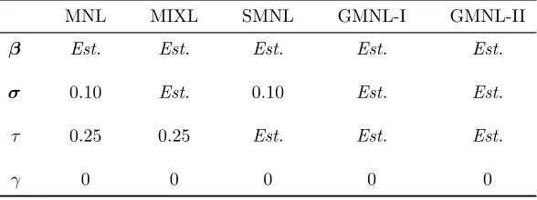
Table 1 summarizes the custom values we combined with each nested model’s
estimates to construct a starting point for GMNL. The MNL starting point draws on
the default setting of the gmnl command and provides a basis for specifying other
starting points. MIXL and SMNL were estimated from the same MNL starting point,
ignoring irrelevant parameters. GMNL-I (GMNL-II) was estimated three times, once
from each of the MNL, MIXL and SMNL starting points, again ignoring irrelevant
parameters; GMNL, in turn, was then estimated once from each of the three potential
GMNL-I (GMNL-II) starting points, though only the best of the three resulting
GMNL solutions is reported below.6
In our view, this implementation of the conventional strategy is representative of what a typical practitioner would do. A few studies commenting on the estimation
process (Greene and Hensher, 2010, p.418; Knox et al., 2013, p.74) only note that
starting values have been obtained from nested models. Also, apart from MNL, each
nested model requires a non-trivial amount of computer time per estimation run,
making it rather cumbersome for the practitioner to experiment with a wide range of
custom values, especially when no relevant guidance exists.
In both case studies, our conventional strategy finds solutions which are different
from what Keane and Wasi (2013) report. Some of our solutions result in higher, and
others worse, log-simulated likelihoods than the corresponding figures in that study. In addition to variations in the process of constructing starting points, such
discrep-ancy may be attributed to different computing environments (Stata and Matlab), for
example in terms of pseudo-random number generation. We do not pursue the exact
source of the discrepancy because our case studies are not intended as replication
exercises. Moreover, even within the Stata computing environment, we find a range
of different solutions from different starting points.
4.2
DE- and PSO-assisted estimation strategies
The DE and PSO algorithms require, as user inputs, the population size P and the
number of generations G. In addition, both algorithms require an initial population
of P candidate solutions that they can improve over G generations.
Following the common practice, we set P=10K where K is the number of
esti-mated parameters. We also set G=10K. The choice of G varies from application to
6In many cases, the GMNL-I (GMNL-II) starting point that led to the best GMNL solution was
application, depending on the nature and purpose of the intended optimization task.7
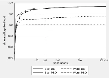
In preliminary experimentation with simulated data sets, we noticed that both
algo-rithms tended to slow down substantially around the 10Kth generation, motivating
our decision to switch to the gradient-based optimization at that point. To illustrate
this slowdown in an empirical context, Figure1plots how a selection of DE and PSO
starting points used in the first case study (Pap Smear) would have varied hadGbeen
set to 420 (or 30K) instead of 140 (or 10K).
The initial population of P solutions is generated as follows. For the GMNL
parameters to be estimated ω = {β, τ , γ,σ}, consider the lower and upper bounds given byl={bM N L,0,0,0}andu={3×bM N L,2,1,1.5×bM N L}, wherebM N L is the vector of the MNL estimates and 0is the K-vector of zeros. For each initial solution,
each element of ω is independently drawn from a uniform variable lying between the
corresponding elements of land u.
The updating process of each algorithm requires two tuning parameters as
ad-ditional user inputs: amplification factor F and cross-over probability Cr in case
of DE, or the acceleration constant C and the inertia weight D in case of PSO.
We follow Gilli and Schumann (2010) in experimenting with 16 pairs, or
configu-rations, of those tuning parameters per algorithm: a DE configuration is in F =
{0.2,0.4,0.6,0.8} × Cr = {0.2,0.4,0.6,0.8}, while a PSO configuration is in C =
{0.5,1.0,1.5,2.0} ×D = {0.5,0.75,0.9,1.0}. The resulting configurations are spaced broadly enough to provide indicative evidence for future applications on what
tun-ing parameter values could be narrowly searched over for further fine-tuntun-ing of each
algorithm.
Since the updating process is partly random, different DE or PSO starting points
would result from the same configuration when different random number seeds are
specified for initialization. We have obtained 48 DE starting points and 48 PSO
starting points, by restarting each configuration three times from the same set of
three seeds. In other words, the same set of three different initial populations has been used to obtain the three starting points associated with each configuration of
each algorithm.
7For example, when optimizing a function with a known global optimum, it may be left unspecified
4.3
Results: Pap Smear
In this data set, each of 79 individuals faced 32 choice scenarios consisting of two
options, namely get a Pap Smear test or not. These options are described by 6
different attributes, including the alternative-specific constant (ASC) for the get-test
option. Estimating the mean (β) and standard deviation (σ) of the canonical random
coefficient on each attribute results in 14 GMNL parameters.
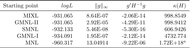
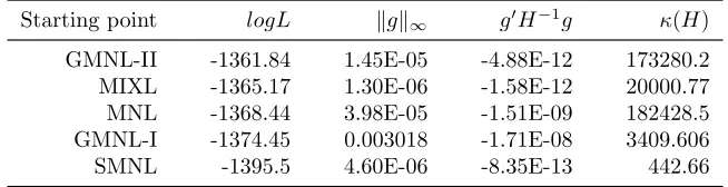
Table 2reports in descending order the simulated log-likelihood values (logL
here-after) of the solutions obtained by applying the conventional strategy, along with the
usual diagnostics for checking convergence to a local optimum. Stata classifies all
solutions as “converged”, implying that the Hessian (H) is negative definite and the weighted gradient norm (g0H−1g) is smaller than -1E-5 in magnitude. Further
inspec-tion suggests that only the MNL-based soluinspec-tion gives warning signs: the inf-norm of
the gradient (kgk∞) deviates far way from zero and the Hessian condition number (κ(H)) exceeds one over the square root of Stata’s machine precision. But this is the worst solution which is unlikely to be reported by a practitioner who tries alternative starting points.
The best solution results in logL of -931.065, which is somewhat higher than -934
in Keane and Wasi (2013). It is also a type of local maximum which practitioners
may find particularly convincing as a candidate for the global maximum, because it
can be reached from two different starting points, namely MIXL and GMNL-II.8 The
negligible difference between their convergence diagnostics arises because the
MIXL-based estimates differ marginally from the GMNL-II-MIXL-based estimates, in or after the
fifth decimal place.
The DE- and PSO-assisted estimation strategies find several solutions which im-prove on the best conventional solution. The best solution is a DE-assisted one,
resulting in logL of -925.378. Table A1 in Appendix reports the logL results from all
3 starts of 16 configurations of each algorithm. The main features of those results may
be summarized as follows. 16 of 48 DE-assisted solutions (35%) result in logL greater
than -931.065, ranging from -928.034 to -925.378. Considering that some of the 48
solutions include those resulting from configurations not well-suited to the present
application, a prima facie case exists that the DE-assisted strategy is a practically
useful complement to the conventional strategy. In contrast, only 3 out of 48
PSO-8Both MNL and MIXL starting points led to the same GMNL-II solution that is used as the
assisted estimation runs (6%) result in an improved solution, ranging from -926.671
to -926.308.
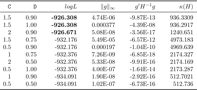
Another practically attractive feature of the DE-assisted solutions is clearer
in-dicative evidence on which configurations are likely to work well. Table 3reports the
top ten logL values found with the aid of each algorithm. A qualitative direction for
fine-tuning the DE configuration to the present application would be “try a big change
to the parameter estimates, but accept the resulting change only occasionally.” No
similar direction emerges in case of PSO, as the top ten solutions are associated with
a wider range of configurations.
To be specific, the top ten DE-assisted solutions are overly represented by config-urations specifying a large amplification factorF (0.6 and 0.8) and a small cross-over
probability Cr (0.2 and 0.4). When restricting attention to the four implied
configu-rations, 9 out of 12 DE-assisted estimation runs (75%) find an improved solution, and
4 of those 9 runs reach the highest logL of -925.378. In contrast, a small F (0.2 and
0.4) appears not well suited, regardless of the accompanying Cr: only 2 of such 28
DE-assisted runs find an improved solution, none of them reaching the highest logL.
The highest logL has been reached from 6 different DE starting points and displays
appropriate convergence diagnostics. Of course, as in the case of the best conventional
solution, such repeatability does not imply that the underlying solution is the global maximum. Verifying that a particular solution is the global maximum is considered
to be beyond the scope of our study because, as far as we are aware, no definitive
guideline exists on how such verification is to be performed. We have, however,
verified that the best conventional solution is not the global maximum. Our present
and subsequent analysis focuses on the consequences of basing an empirical analysis
on the best conventional solution when a DE- or PSO-assisted solution is capable of
achieving a higher logL.
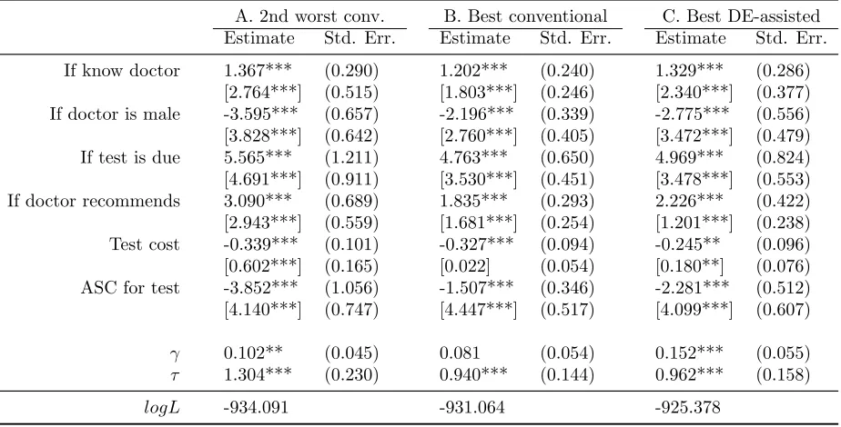
Table 4 reports the second-worst and best conventional solutions, along with the
best DE-assisted solution. The second-worst conventional solution (Solution A) re-sults from the GMNL-I starting point, and is the worst one out of conventional
solu-tion with acceptable convergence diagnostics. In terms of logL, the best convensolu-tional
solution (Solution B) gains over Solution A by some 3 points, and there are marked
differences between the coefficient estimates: the mean of “ASC test”, in particular,
is about 2.5 times larger in Solution A than in Solution B (-3.85 vs. -1.51) and many
There are less pronounced differences between the best DE-assisted solution
(So-lution C) and the best conventional so(So-lution (So(So-lution B), despite that C improves
on B by 6 logL points, or twice as much as B improves on A. The main difference
between the solutions is that while solution B supports simplifying the model to a
more parsimonious GMNL-II model with a fixed test cost coefficient, solution C does
not support such a simplification as both the estimate ofγ and the standard deviation of the cost coefficient are significant and non-trivial. The remaining differences are
not such that it becomes immediately obvious from simple inspection whether
policy-relevant statistics derived from these solutions, such as the median willingness-to-pay
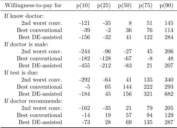
(WTP) and the predicted choice probability, would be substantively different.9 To facilitate further comparisons, Table 5 reports selected percentiles of WTP
distributions simulated from solutions A, B and C. As expected from the earlier
comparison of A with B, these two solutions imply quite different median WTP,
the primary statistic on which practitioners are likely to focus (e.g. Small et al.,
2005). The implied WTP distributions of B and C, on the other hand, are only
slightly different at the median. The main difference between those two solutions
is that due to heterogeneity in the cost coefficient which is only picked up by C,
the interpercentile ranges of WTP are much more pronounced for C than B.10 As a result, conclusions regarding the dispersion of the WTP distribution implied by B may require reconsideration.
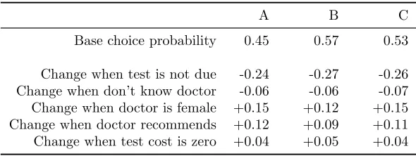
Table 6 compares the three solutions in terms of the predicted changes in the
probability of choosing the Pap Smear test in response to attribute level variations.
The baseline specification of the attribute levels has been motivated by what Johar
et al. (2013, p.1853) find plausible in the Australian context. As in the case of the
median WTP, solutions B and C agree on the substantive conclusions, predicting
changes of similar magnitudes and indicating that under the baseline scenario, the
test is more likely to be chosen than not. In this case, however, solution A also
9The WTP for a specific attribute is the utility coefficient on that attribute divided by the
absolute value of the utility coefficient on the price or cost attribute. The WTP distribution can be simulated first by making simulated draws for all utility coefficients according to equation (2), and then computing relevant ratios of those simulated coefficients.
10More specifically, the test cost coefficient is very tightly distributed around its mean in B,
yields almost the same results as the others, apart from that in line with its large and
negative ASC, it predicts a smaller baseline probability of the test (0.45) than B (0.57)
and C (0.53). This robustness may stem from the same source as the difficulties of
finding the global maximum, namely that different combinations of parametric values
lead to similar probabilities or likelihoods.
4.4
Results: Pizza A data
In this data set, each of 178 individuals faced 16 choice scenarios consisting of two
hypothetical pizza delivery services. These services are described by 8 different
at-tributes. Estimating the mean and standard deviation of the canonical random
coef-ficient on each attribute results in 18 GMNL parameters.
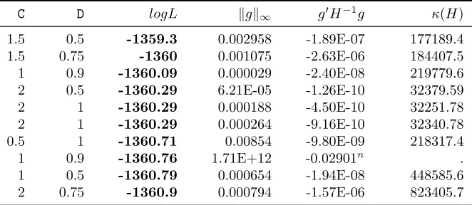
Table7reports logL values attained by the conventional solutions. The MIXL and GMNL-II starting points again turn out to be two best conventional starting points.
But this time only GMNL-II leads to the highest logL of -1361.84, which lies above
-1372 reported in Keane and Wasi (2013).11 All conventional solutions, including the
worst one, display acceptable convergence diagnostics.
The full set of the DE- and PSO-assisted estimation runs are reported in Appendix
Table A2, and the results agree with the Pap Smear results on two broad conclusions.
First, the best solution is obtained by the DE-assisted strategy and attains logL of
-1356.80. Second, the DE-assisted strategy outperforms the PSO-assisted strategy in
terms of finding a solution improving on the best conventional solution, even though this time the PSO-assisted strategy does better than in the Pap Smear case study:
42% or 20 out of 48 DE-assisted solutions, and 23% or 11 of 48 PSO-assisted solutions,
improve on the best conventional solution.
The current results, however, are quite different from the previous results in one
important dimension. 11 DE-assisted solutions (23%) and 4 PSO-assisted solutions
(8%) have been declared “not converged” by Stata, because the associated Hessian is
not negative definite and/or g0H−1g exceeds the tolerance level. No solution in the Pap Smear case study displays this issue.
More importantly, the clear sign of non-convergence is present in the four best solutions we have obtained. All these solutions are in the “DE-assisted” panel of
Table 8, which reports the 10 best DE-assisted and PSO-solutions. Both kg k∞ and
g0H−1g of the four solutions evidently deviate from zero, and in the case of the three
best solutions κ(H) is negative meaning that the Hessian is not negative definite. Since these are symptoms of an empirically underidentified model, we followed the
advice of Chiou and Walker (2007) for further inquiry. Specifically, we re-estimated
the model by using as starting point the best conventional solution, and making
10,000 draws to simulate the log-likelihood function. As Chiou and Walker point
out, using a larger number of draws unmasks empirical underidentification: while the
best conventional solution displays acceptable convergence diagnostics at 500 draws,
the new estimation run failed to attain convergence.12 We note that, in the case of the Pap Smear data, similarly starting an estimation run from the best conventional solution led to convergence within 7 iterations.13 Thus, in the present application, the
use of the DE- and PSO-assisted strategies leads to a practically different implication
from the conventional strategy: namely, that the model needs to be simplified before
the parameter estimates can be readily interpreted.14
Putting the empirical underidentification issue aside, the present case study also
yields more ambiguous guidance on configurations of the DE and PSO algorithms.
As in the Pap Smear application each PSO configuration tends to perform differently
across three restarts, and now the DE configurations also perform somewhat more
erratically. The 10 best DE-assisted solutions in Table 8 vary widely in terms of
Cr, though it still appears to be the case that taking F from {0.6,0.8}, especially 0.6, is a good choice. The full set of results in Table A2 shows that there are a few more runs with configurations involvingF={0.2,0.4}that find an improved solution, on top of the two which already appear in Table 8 (recall that such configurations
performed poorly in the Pap Smear application). We note, however, that restricting
attention to F={0,6,0.8} ×Cr= {0.2,0.4} still seems to be a valid baseline choice: such configurations find an improved solution in 67% or 8 of 12 runs, and encompass
(F,Cr)= (0.6,0.4) which finds an improved solution in all three restarts.
12More specifically, logL rose from -1362.46 to -1353.08 after 31 iterations, at which the Hessian
was not negative definite, and no further change occurred during the next 69 iterations.
13LogL rose from -938.273 to 936.399.
14We found no such evidence of empirical underidentification in a mixed logit model estimated on
5
Further case studies
The results described in the previous section suggest that the DE- and PSO-assisted
estimation strategies can be a useful tool for improving the chance of finding the
global maximum in empirical applications. Between the two strategies, the
DE-assisted strategy appears to be the better choice since it improves on the conventional
solution more frequently and is more consistent in terms of which configurations are
likely to perform well. The best conventional and DE-assisted solutions have led to somewhat (Pap Smear) and quite (Pizza A) different substantive conclusions based
on the estimated GMNL models.
In this section, we explore the applicability of the earlier findings to other
empiri-cal contexts and computational configurations. The discussion is based on additional
sets of estimation results, only a subset of which is reported below for brevity of
pre-sentation. Interested readers are referred to our Online Appendix for other discussed
results.15
5.1
Holiday A data and Mobile Phone data
It is reasonable to ask whether the configurations of DE algorithm which were most
likely to improve on the conventional solution in the previous section (F={0,6,0.8} ×
Cr= {0.2,0.4}) will also perform well in other empirical applications. To examine this question, we have applied the same configurations to estimate GMNL using the
Holiday A and Mobile Phone data sets from Fiebig et al. (2010) and Keane and Wasi
(2013). These data are on individuals’ choices from hypothetical holiday packages and
from hypothetical mobile phones, respectively. The results are encouraging: the
DE-assisted strategy improves on the best conventional solution in 11 out of 12 restarts
(92%) in Holiday A, and in all of 12 restarts in Mobile Phone (100%). Furthermore,
it is interesting to note that in both data sets the (F=0.8, Cr=0.2) configuration repeatedly locates the best solution we have obtained, just like it did in the Pap
Smear application.
The overwhelmingly better performance of the DE-assisted strategy relative to
the conventional strategy may be explained by underlying computational difficulties.
15The Online Appendix can be accessed at:
https://www.dropbox.com/s/nopimkjotwmsvfu/Dec2014_Hole_and_Yoo_Online_Appendix.
The Holiday A and Mobile Phone data sets have 331 and 493 individuals, respectively,
far more than the 79 and 178 individuals in the Pap Smear and Pizza A data sets.
Thus, the present cases require many more person-specific likelihoods be simulated.
In addition, the Mobile Phone data set requires the estimation of more than 10
extra parameters in comparison with the other data sets. With such factors adding
to computational difficulties, the choice of starting values may become even more
important.16
In both data sets, nevertheless, the best conventional solution and the best
DE-assisted solution still show a large amount of agreement on substantive conclusions.
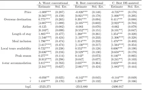
Table 9 report the best DE-assisted solution along with the worst conventional and best conventional solutions for Holiday A, and Table 10 report the corresponding
results for Mobile Phone.17 All three solutions display appropriate convergence
diag-nostics for local maxima in both data sets.
Holiday A yields qualitatively similar results to Pap Smear in the previous
sec-tion. The best DE-assisted solution achieves a 22.96-point higher logL than the best
conventional solution (logL = -2490.92 vs -2513.88), and this difference is much larger
than the 9.3 points that the latter gains over the worst conventional solution (logL
= -2523.27). Yet, in terms of the parameter estimates, the difference between the
best DE-assisted and best conventional solutions is not as evident as that of the best and worst conventional solutions, apart from that the best DE-assisted solution
finds much less coefficient heterogeneity for ‘Airline’ and more for ‘Peak season’. The
comparisons of simulated WTP distributions lead to the same conclusion.
In Mobile Phone, it is also the case that the best DE-assisted solution gains many
more logL points over the best conventional solution than the latter gains over the
worst conventional solution. The logL values of the three solutions are 3937.97,
-3951.66 and -3954.89 respectively. The comparisons of the parameter estimates are
less straightforward in this application as it involves many more parameters, most
16This explanation invites the question of why the DE-assisted strategy was found to perform
worse in the Pizza A application that involves more individuals and parameters. One possibility is that it is an anomaly due to empirical underidentification. We note that when GMNL is re-estimated by using 10,000 simulated draws and starting from the best conventional solution at 500 draws, the estimation run achieves convergence within a few iterations in both the Holiday A and Mobile Phone data sets, much as in the Pap Smear data set.
17Keane and Wasi (2013) report the logL values of -2512 for Holiday A and -3966 for Mobile
of which are statistically insignificant at all conventional levels. It is, nevertheless,
evident that the best DE-assisted solution stands out from both the best and worst
conventional solutions. Several standard deviation estimates are significant only in
the best DE-assisted solution, and often larger in magnitude than the corresponding
estimates in one or both of the conventional solutions. Thus, if significant standard
deviations are used to gauge market segments to which particular mobile phone
fea-tures may appeal, the best DE-assisted solution can lead to quite different marketing
decisions than the best conventional solution.
We conclude this subsection with remarks on the PSO-assisted strategy. The
previous section suggests that the performance of various PSO configurations tends to be erratic across restarts. In the absence of clearer evidence on suitable baseline
configurations, we have applied those drawn from C={1.5,2.0} ×D={0.75,0.9} to the Holiday A and Mobile Phone data sets by restarting each of the resulting four
configurations three times. The results again suggest that the DE-assisted strategy
outperforms the PSO-assisted strategy: the latter improves on the best conventional
solution less frequently (4 out 12 restarts in Holiday A and 7 out of 12 restarts in
Mobile Phone), and the best PSO-assisted solution achieves worse logL than the best
DE-assisted solution (-2507.70 in Holiday A and -3949.79 in Mobile Phone).
5.2
All data sets: comparison with the random perturbation
strategy
Our use of the DE and PSO algorithms is essentially a sophisticated method for
obtaining a suitable random starting point. As the non-identical results across the
three starts from the same configurations illustrate, each algorithm works by refining
the initial population of several random starting points repeatedly to produce one
improved random starting point. In addition, at least in the Pap Smear and Holiday A data sets, the best DE-assisted and best conventional solutions resemble each other
closely in terms of parameter estimates. This proximity, together with the inherent
randomness of the DE starting points, leads to the question of whether using a
ran-domly perturbed version of the best conventional solution as starting point could be
considered as an effective substitute for the DE-assisted estimation strategy.
To address this question, we have applied the following random perturbation
conven-tional solution, a draw is made from a uniform distribution over ±4 standard errors
of the estimate. A perturbed starting value for the relevant parameter is obtained by
adding up the estimate and the uniform draw. Then, a new random starting point
is specified as a vector of the perturbed starting values for all parameters. 20 such
starting points have been generated for each data set, and used to estimate GMNL
via the Newton-Raphson algorithm.
Table 11reports the best five logL values resulting from the 20 perturbed starting
points. The results suggest that while the perturbation strategy may sometimes
be useful in checking for the robustness of the best conventional solution, it cannot
readily locate or improve on the best DE-assisted solution. In the Pap Smear data, all five best solutions coincide with the best conventional solution, while in the Pizza
A data, all solutions are worse than the best conventional solution. In the Holiday A
data, all five best solutions improve on the best conventional solution, but even the
very best perturbed solution gains only 1.41 points in terms of logL, much smaller
than the best DE-assisted ’s gain of 22.96 points. In the Mobile Phone data, the
perturbation strategy again turns out to be useful in detecting the inadequacy of the
best conventional solution, which is beat by all five best perturbed solutions, but not
capable of locating or outperforming the best DE-assisted solution.
5.3
Pap Smear and Pizza A: 20 starts
Our findings so far have suggested that good baseline configurations of the DE al-gorithm can be drawn from F = {0.6,0.8} ×Cr = {0.2,0.4}. As explained earlier the starting point for the algorithm is randomly determined, and we now explore the
robustness of the configurations from an alternative angle by restarting each of the
four configurations using twenty different random number seeds instead of three as in
the previous analysis. For this purpose, we use the Pap Smear and Pizza A data sets
whose smaller sizes make them more amenable to a large number of estimation runs.
In each data set, the results over 80 restarts confirm that the performance of these
configurations is consistently good. In the Pap Smear data, 49 out of 80 restarts
(61.25%) improve on the best conventional solution. The frequency is smaller than the 75% (over 12 comparable restarts) found earlier, but still covers the majority
of cases. In the Pizza A data 62 out of 80 restarts (77.5%) improve on the best
Table 12reports the ten best DE-assisted solutions found from the 80 restarts in
each data set. The results for the Pap Smear data suggest that (as in the case of the
best conventional solution) repeatedly finding a particular maximum is not a reliable
sign that it is the global maximum. Now, there are two new maxima at the logL values
of -924.359 and -924.788, both of which are higher than the logL of -925.378 in the best
DE-assisted solution found in the previous section, which was reached four times out
of the 12 restarts from the configurations under consideration. An interesting aspect
of the parameter estimates at -924.359 is that like the best conventional solution, the
standard deviation of the cost coefficient is small and insignificant, in contrast with
the “best DE-assisted” solution of the previous section where it is significant. Given the difficulties of verifying the global maximum in empirical work, it appears prudent
to report all main differences across several maxima found in estimation runs, as
Knittel and Metaxoglou (2014) recommend in the context of the
Berry-Levinsohn-Pakes method of demand estimation.
5.4
All data sets: mixed logit case studies
While our focus so far has been on GMNL, the presence of several local maxima is
a feature of all random parameter logit (RPL) models. Our DE- and PSO-assisted
estimation strategies can be readily adapted to the estimation of other RPL models,
and in this section we explore whether the above findings are generalizable to the RPL
model with normally distributed coefficients and no scale heterogeneity (MIXL). This model is the best known and arguably most widely estimated RPL specification, to
the point where the generic term “mixed logit” is often used to describe this particular
model (e.g. Fiebig et al., 2010). For the four data sets in use, the preferred MIXL
specification of Fiebig et al. (2010) constrains the off-diagonal elements of Σto zero,
like their preferred GMNL specification. We take their preferred MIXL specification
as given and estimate the mean (β) and standard deviations (σ) of the normally
distributed coefficients.
For each data set, several MIXL solutions have been obtained using the same
tuning parameter values for the DE and PSO algorithms as in the previous sections. Only one conventional solution has been obtained in this case since using the MNL
coefficients as starting values is likely to be the most common strategy for estimating
starting values used in estimating the MIXL specification of interest here, presumably
because the underlying optimization task may be perceived as numerically simple in
that the postulated utility function is linear in parameters and convergence to local
maxima can be achieved from a wide range of starting values.18
The results across the four data sets suggest that our earlier findings on the
perfor-mance of DE- and PSO-assisted strategies are not exclusively associated with GMNL
(see the Online Appendix for detailed results). Despite the relative numerical
sim-plicity of the MIXL optimization task, the DE- and PSO-assisted strategies perform
better than both the conventional strategy and the random perturbation strategy.
The DE-assisted strategy still outperforms the PSO-assisted strategy in that the for-mer locates solutions improving on the conventional solution with a greater frequency,
and it also finds the best solution out of the ones we have obtained. Moreover, the
DE-assisted results from the Pap Smear and Pizza A data sets show that our preferred
baseline configurations based on Section 4 are well-suited to the MIXL specification
too.
One notable difference when comparing the MIXL and GMNL results is that the
MIXL solutions at various local maxima show much greater agreement in terms of
policy-relevant statistics than the GMNL solutions do. The conventional solution, the
best solution from 20 randomly perturbed starting points and the best DE-assisted solution can be found in the Online Appendix. Presumably because the random scale
factor, which can influence all other parameters, is absent in MIXL, all three sets
of estimates look very similar and produce almost the same percentiles of the WTP
distribution.
6
Conclusion
It is well known that the log-likelihood function of the random parameter logit model may feature multiple maxima, and that the final estimates may be sensitive to the
choice of starting values. Only limited documentation and practical guidance exist,
however, on the issue of which starting values to use in the estimation process. In this
paper, we have proposed an estimation strategy which uses the differential evolution
18This contrasts with, for example, the cases of GMNL and an RPL model allowing for
(DE) and particle swarm optimization (PSO) algorithms to obtain starting values.
These heuristic algorithms search over the parameter space much more
comprehen-sively than gradient-based algorithms, and can be expected to locate a point close
to the global maximum more easily. We have applied this strategy in four different
empirical data sets to estimate the generalized multinomial logit model (GMNL),
a random parameter logit model featuring both scale and coefficient heterogeneity.
The objectives of our empirical applications have been to examine how the DE- and
PSO-assisted strategies perform relative to each other as well as to common strategies
that most practitioners are likely to be currently following, and also to investigate
whether there is a particular configuration of each algorithm which repeatedly results in satisfactory performance. For the common strategies, we have considered (i) the
conventional strategy of starting from the estimated special cases of the final model
and (ii) the random perturbation strategy of taking random starting points around
the best solution found via (i).
Our findings suggest that the DE-assisted strategy can be a very effective tool to
diagnose the adequacy of the modeling results obtained using the conventional
strat-egy. In all four data sets, the DE-assisted strategy has located solutions which attain
higher log-likelihood values than what the PSO-assisted strategy and the conventional
strategy have found. Those improved solutions have been obtained with high enough empirical frequencies to suggest that a small number of DE-assisted estimation runs
would be sufficient for detecting the potential inadequacy of a currently preferred
conventional solution. In contrast, the random perturbation strategy has failed to
improve on the best conventional solution in two of the four data sets, in addition to
resulting in worse solutions than the best DE-assisted solution in all data sets.
The best DE-assisted solution has always achieved a larger gain in the log-likelihood
over the best conventional solution than the latter has achieved over the worst
con-ventional solution. These larger gains make it interesting to note that in two of the
four case studies (Pap Smear and Holiday A), the best DE-assisted and best conven-tional solutions overlap more in terms of substantive conclusions, such as the median
willingness-to-pay, than the best and worst conventional solutions do. It therefore
seems possible for the policy implications of a carefully selected conventional solution
to remain valid even when the solution is at an inferior local maximum.
An attractive feature of our heuristically assisted estimation strategy is its