Angle of Incidence Effects on Far-Field Positive and Negative Phase Blast Parameters

by

Sam E. Rigby, Stephen D. Fay, Andrew Tyas, James A. Warren and Sam D. Clarke

Reprinted from

International Journal of

Protective Structures

Volume 6 · Number 1 · March 2015

*Corresponding author. Tel.: + 44 (0) 114 222 5724. Email address: [email protected]

Angle of Incidence Effects on Far-Field

Positive and Negative Phase Blast

Parameters

Sam E. Rigby1,_{*, Stephen D. Fay}1,2_{, Andrew Tyas}1,2_,

James A. Warrena,b_{and Sam D. Clarke}a

1_{Department of Civil & Structural Engineering, University of Sheffield,}

Mappin Street, Sheffield, S1 3JD, UK.

2_{Blastech Ltd., The BioIncubator, 40 Leavygreave Road, Sheffield,}

S3 7RD, UK.

Received on 2 Sept 2014, Accepted on 18 Nov 2014

ABSTRACT

The blast overpressure acting on a rigid target is known to vary between the normally reflected overpressure and the incident overpressure as a function of the angle between the target and the direction of travel of the blast wave. Literature guidance for determining the exact effects of angle of incidence are unclear, particularly when considering the negative phase. This paper presents the results from a series of well controlled experiments where pressure transducers are used to record the pressure-time history acting on the face of a large, rigid target at various angles of incidence for varying sizes of hemispherical PE4 charge and stand-off distances. The test data demonstrated remarkable repeatability, and excellent agreement with semi-empirical predictions for normally reflected overpressures. The oblique results show that peak overpressure, impulse and duration are highly dependent on angle of incidence for the positive phase, and are invariant of angle of incidence for the negative phase.

Keywords: Angle of Incidence; Blast; Experimental Validation; Negative Phase; Positive Phase; UFC-3-340-02

NOMENCLATURE

b decay of exponential pressure-time curve

i_r reflected positive phase specific impulse reflected negative phase specific impulse

i_so incident positive phase specific impulse incident negative phase specific impulse

K Hopkinson-Cranz length scale factor

p₀ ambient pressure

p_r reflected overpressure

− iso

p_r,max peak reflected overpressure

p_r,min peak reflected underpressure

p_so,max peak incident overpressure

p_so,min peak incident underpressure

R distance from charge centre (stand-off)

R_Gi distance from charge centre to gauge i, where i=1:4

t time

t_a time of arrival of blast wave

t_d positive phase duration negative phase duration

W charge mass

Z scaled distance θ angle of incidence

θGi angle of incidence for gauge i, where i=1:4

1. INTRODUCTION

A large amount of energy is released after the detonation of a high explosive material, causing rapid expansion of the surrounding air and generating a blast wave. As this blast wave propagates outwards away from the source of the explosion, the compressible nature of air causes the blast wave to ‘shock up’, resulting in an effectively discontinuous increase in pressure, density and energy of the travelling shock [1]. The pressure profile associated with a blast wave takes the form of the idealised pressure-time history shown in Figure 1: ambient pressure (p₀) is recorded until the arrival time of the blast wave (t_a), followed by a sharp rise to peak pressure and temporal decay back to ambient conditions. Immediately after the end of the positive phase (the duration of which is defined as t_d) comes a subsequent period of below-atmospheric (‘negative’) pressure caused by an inertial response and over-expansion of the previously compressed air. The duration over which negative phase pressures are acting is defined as . The term ‘overpressure’ refers to the pressure increase above normal atmospheric conditions caused by the blast wave, which is relevant for design purposes. Similarly the term ‘underpressure’ refers to blast pressures which are below atmospheric conditions.

− t_d

Figure 1. Idealised pressure-time profile for a blast wave i_so

i_r p_so

p_r p

p_r,max

p_so,max

p_so,min p_r,min

i_so− i_r−

−

t_a t_d t_d

If a blast wave is propagating through free air, the blast wave is known as an incident wave, and the peak positive overpressure and negative phase underpressure are defined as

p_so,maxand p_so,min respectively. Here, the peak overpressure and underpressure are defined as the maximum or minimum pressure value relative to atmospheric conditions. The impulses associated with the positive and negative phase, i_soand , are the temporal integral of the blast overpressures over the positive and negative phase respectively. If a blast wave impinges normally onto a rigid target, conservation of mass, momentum and energy at the interface results in an increase in the blast pressures, which are given the subscript _rto denote ‘reflected’ values. The reflected overpressure is at least twice the magnitude of the incident overpressure for weak shock conditions, but can be significantly higher for stronger shocks.

1.1. PREDICTING BLAST LOADS ON STRUCTURES

Kingery and Bulmash [2] provide a semi-empirical method for predicting blast wave parameters based on a compilation of a wide range of test data and computer analyses. The blast parameter relationships derived from this body of work are usually presented graphically as scaled distance relationships, where the scaled distance, Z, is given as

(1)

where Ris the distance (or stand-off) from the explosive to the point of interest (m) and W

is the mass of explosive (kg of TNT equivalent). Hopkinson-Cranz scaling states that similarity exists between the blast waves produced at identical scaled distances from two explosive charges of similar geometry but different sizes [1]. That is, the blast pressure profile at a distance of Rfrom an explosive mass Wwill be similar to the blast pressure at a distance of KRfrom a mass of K3_{W, where Kis an arbitrary length scale factor. In this pair} of scenarios, the peak overpressure will be the same, whilst the time-scales will be different by the scale factor K. The scaled distance relationships therefore have a wide range of application and form the basis of literature guidance including the US Department of Defence Design Manual UFC-3-340-02, Structures to Resist the Effects of Accidental Explosions[3], and the computer code ConWep [4].

The angle of incidence between a target and a blast, θ, is defined as the angle between the outward normal of the reflecting surface and the direct vector from the explosive charge to that point [5]. If θ= 0.0°, the surface will be subjected to the fully reflected overpressure, and if θ= 90°, the blast wave will have incident values as it is propagating parallel (or ‘side-on’, hence incident values having the subscript _so) to the target surface. The blast overpressure for any oblique blast wave impinging at an angle of incidence between these two extremes will comprise some combination of the reflected and incident values.

For positive phase parameters, the effect of angle of incidence is generally well understood, however the guidance in the literature appears contradictory. Positive phase reflection coefficients can be determined graphically – from curves based on either semi-empirical data (Figures 2-193 and 2-194(a) and (b) in [3], repeated here in Figures 2(a) and (b)) or analytical solutions of shock equations (Figure 5-8 in [6]) – or by using simplified expressions. Randers-Pehrson and Bannister [7] suggest a trigonometric relation for calculating the oblique blast overpressure as a function of p_r,max, p_so,max and θ, and Remennikov [5] suggests using full reflected values for θ ≤45°. It is known that the angle of incidence affects the pressure and the impulse differently. Furthermore, for θ > 45°,

=

Z R

W1/3

Figure 2. (a) Reflection coefficient versus angle of incidence, (b) oblique scaled impulse versus angle of incidence (adapted from Figures 2-193 and 2-194(a)/(b) in [3]), and (c), formation of the Mach stem

0 14 (a)

(b)

(c) 12

10

8

Reflection coef

ficient,

pr,

max

/p

so,max

6

4

2

0

10 20 30 40

Angle of incidence, θ (°)

50 60 70 80 90

0 104

103

102

101

Scaled oblique impulse (kPa.ms/kg

1/3

)

10 20 30 40

Angle of incidence, θ (°)

50 60 70 80 90

34,500

p_so,max (kPa)

20,700 13,800 6,890 2,760 1,380 689 345 138 68.9 34.5 13.8 6.89

34,500 20,700 13,800 6,890 2,760 1,380 689 345 138 68.9 34.5 13.8 6.89

Charge

θ

Incident wave

Reflected wave

Mach stem

Target

the reflected shock front and propagating incident shock front will coalesce to form the Mach Stem [6], which can lead to large amplification in the oblique pressure, often exceeding the normally reflected overpressure at that point. This phenomenon is illustrated schematically in Figure 2(c).

The negative phase is frequently ignored in the literature, despite it having been shown that the negative phase can be of significance for flexible structures at relatively large scaled distances [8-10]. Because of its perceived lack of importance, there has been no research into the effect of angle of incidence and there remains very little guidance for quantifying the negative phase for oblique reflection. As stated in the methodology manual for the US Army Blast Effects Design Spreadsheet, SBEDS [11]:

‘so little is known about the negative phase blast load, including the effect of angle of incidence… the lack of a well-validated method for predicting the negative phase blast load is a legitimate reason for using the traditional approach of ignoring negative phase blast load when calculating component response.’

Accordingly, SBEDS recommends using the full reflected negative phase underpressure for θ ≤45° and the full incident negative phase underpressure for θ >45°. There remains an opportunity, therefore, to study oblique blast waves with a view to providing more rigid guidance for researchers and practising engineers. This paper presents the results from a series of well controlled experiments to determine the effects of angle of incidence on positive and negative phase blast parameters.

2. EXPERIMENTAL SETUP

A series of experimental trials was conducted at the University of Sheffield Blast & Impact Laboratory in Buxton, Derbyshire, UK. Four Kulite HKM pressure gauges were embedded flush to the surface of small steel plates which were affixed to the outer surface of a large, reinforced concrete bunker wall using M10 bolts such that the bolts sat flush to the face of the steel plates, maintaining a smooth, regular reflecting surface for the blast wave to propagate over. The primary pressure gauge, labelled G1, was located at ground level. Two subsequent pressure gauges, G2 and G4, were also located at ground level, 2 m and 3 m along the bunker wall away from G1. A final pressure gauge, G3, was situated in line with G1, 2 m vertically above it. The pressure gauge location can be seen in Figure 3.

Hemispherical PE4 explosive charges were placed on a 50 mm thick steel anvil, in line with G1. The charges sat on a level, flat concrete ground slab which was swept clean after each test, following the approach set out in Ref. [12]. This enabled the detonation to be considered as a hemispherical surface burst propagating over a rigid ground surface. Pressure was recorded using a TiePie Handyscope 16-Bit Digital Oscilloscope at a sample rate of 200 kHz, triggered via a voltage drop in a breakwire embedded in the charge periphery to synchronise the recordings with the detonation. The distance from the centre of the charge to the bunker wall was measured for each test using a Hilti laser range meter and was triangulated against two points on the bunker wall to ensure the charge was orthogonal to G1.

G4

G2

2 m G3

1m

2m

GI

R_G1 R_G2

R_G4

R_G3 θ_G3

θ _θ

G2

G4

Figure 3: Pressure gauge location and general test arrangement

W₁

(W₁,W₂,W₃)

W2

W3

Z

1 m R_G4

RG2

RG1

2 m Z

Z

Figure 4: Choice of charge masses to achieve similar scaled distances at different angles of incidence

(2)

where W₁, W₂ and W₃ are the charge masses used in tests 1, 2 and 3, R_G1 is the normal distance from the explosive to G1, and R_G2and R_G4are the slant distances from the explosive to gauge G2 and G4 respectively, as per Figure 3. If the normal distance is constant for the

= = =

R W

R W

R

W Z

( ) ( ) ( )

G1 G G

1 1/3

2 2

1/3 4 3

three tests, then Equation 2 can be rearranged to express W₂and W₃in terms of W₁and R_G1, as in Equation 3.

and (3)

For normal distances of 4 m and 6 m, Equation 3 gives ratios of W₁: W₂: W₃as 1.00: 1.40: 1.95 and 1.00: 1.17: 1.40 respectively. This arrangement maximises the potential of the data to yield useful scaled distance-angle of incidence relationships. Tests were also conducted at 2 m normal stand-off to give angles of incidence ≥45°. A summary of the test plan is given in Table 1, which shows normal and slant scaled distances and angles of incidences for each test. A total of 18 tests were conducted. Scaled distances are in terms of kg of TNT equivalent, using an equivalence factor of 1.20 for PE4 as determined previously by the authors [13, 14].

3. CURVE FITTING TO EXPERIMENTAL DATA

A short duration of artificial ringing following the shock front is a common feature of experimental blast trials [9, 15] and the peak recorded pressure is often a misrepresentation of the applied blast pressure. Because of this, and the tendency for the signals to display some degree of electrical noise, the experimental data was processed using curve fitting techniques. The positive phase of the temporal variation of blast overpressure, p_r(t), can be represented by the ‘modified Friedlander equation’ [16], shown in Equation 4.

(4)

where tis time, bis a coefficient that controls the decay of the exponential curve and p_r,max

and t_d are the peak reflected overpressure and positive phase duration as introduced

= ⎛ ⎝ ⎜ ⎜⎜ ⎞ ⎠ ⎟ ⎟⎟ = + ⎛ ⎝ ⎜ ⎜ ⎜⎜ ⎞ ⎠ ⎟ ⎟ ⎟⎟

W W R

R W R R 2 G G G G 2 1 2 1 3 1 1 2 2 1 3 = ⎛ ⎝ ⎜ ⎜⎜ ⎞ ⎠ ⎟ ⎟⎟ = + ⎛ ⎝ ⎜ ⎜ ⎜⎜ ⎞ ⎠ ⎟ ⎟ ⎟⎟

W W R

R W R R 3 G G G G 3 1 4 1 3 1 1 2 2 1 3 = ⎛ − ⎝⎜ ⎞ ⎠⎟ −

p t p t

t e

( ) 1

r

d bt

td

r,max

Table 1. Summary of test plan

R_G1 W Z(m/kg1/3_{) θ (°)}

Test (m) (g PE4) G1 G2 G3 G4 G1 G2 G3 G4

1-2 2 250 2.99 4.23 4.23 5.39 0.00 45.0 45.0 56.3

3-4 2 210 3.17 4.48 4.48 5.71 0.00 45.0 45.0 56.3

5-6 4 350 5.34 5.97 5.97 6.68 0.00 26.6 26.6 36.9

previously. A Friedlander curve was fit to the positive phase of the experimental data, where the positive phase duration was estimated from the pressure readings and a least-squares approach was adopted to determine the values of band p_r,max which best represented the data. Data for the first ˜25% of the positive phase was omitted to prevent the sensor ringing from influencing the curve fit. This procedure was adopted for all tests with the exception of Tests 1-4, where the peak overpressure for the oblique shots (G2, G3 and G4) was estimated from the pressure readings because of the presence of the Mach Stem, which resulted in a non-regular decay of the positive phase.1 _{The arrival time was given directly by the} experimental recordings. Numerically integrating the recorded pressure time history may be sensitive to sensor ringing, hence the positive phase impulse was determined from the integral of the fitted Friedlander equation, shown in Equation 5.

(5)

Similarly, a least-squares curve was fit to the recorded data from the negative phase. The cubic expression of Granström [17], given in Equation 6, was used to approximate the negative phase based on the findings from previous validation work conducted by the current authors [9].

(6)

Again the negative phase duration, , was estimated from the pressure readings and the peak negative phase underpressure, p_{r, min}, was given by the curve fit. To construct an idealised negative phase from the experimental recordings, any features of the second shock were removed from the data set used for the curve fit, as was data which was judged to have been recorded after the arrival of the diffraction wave from the top edge of the bunker wall. Estimations of negative phase duration were adjusted to take this into account. The idealised negative phase impulse, therefore, is given as the integral of Equation 6, which is shown here in Equation 7.

(7)

4. EXPERIMENTAL RESULTS

The compiled experimental results are presented in this section, with time and impulse values scaled by W−1/3 _{to allow for comparison with semi-empirical predictions. Positive} phase parameter predictions are taken directly from ConWep [4], and negative phase parameter predictions are taken from relationships developed by the current authors (Equations 3 and 4 in Ref. [9]). Both are based on data presented in UFC-3-340-02 [3].

− t_d =− ⎛ − ⎝ ⎜ ⎞ ⎠ ⎟ −⎛ − ⎝ ⎜ ⎞ ⎠ ⎟ − −

p t p t t

t

t t t

( ) 27

4 1 r r,min d d d d 2

∫

i p t dt( ) 9p t

16 r r t t t r,min d d d d

∫

i p t dt p t

b b e

( ) ( 1 )

r r

t

r max d b

0

, 2

d

1_{For these tests, the angles of incidence were 45°or greater, meaning that the Mach stem had formed by the time}

Whilst the complete data set is mainly presented graphically in this section, tabulated parameters for each test are available in Tables A1, A2 and A3 in the Appendix.2_{It is the} authors’ intention to make these results available in the literature as a complete data set for use in validation of numerical modelling approaches and benchmarking of physical test data. Figure 5 shows scaled arrival times versus scaled distance for all tests. The mean arrival time for each set of repeat tests is presented in Figure 6, normalised against the semi-empirical predicted arrival time.

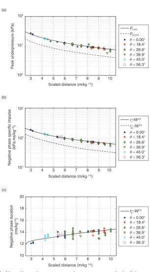
Scaled positive phase parameters – i.e. pressure, impulse and duration – are presented in Figure 7 versus scaled distance. Reflected predicted values are shown by the solid lines, and incident values by the broken lines. Again, the mean value from each set of repeat tests has been normalised against the semi-empirical prediction, where the pressure and impulse are normalised against the full reflected values at that scaled slant distance. Normalised positive phase values are shown in Figure 8. Scaled negative phase parameters are shown in Figure 9, with normalised values shown in Figure 10. Again, oblique experimental parameters have been normalised against fully reflected parameters to show the effects of angle of incidence.

102

101

100

3 4 5 6 7

Scaled distance (m/kg 1/3₎

t_a/W1/3

θ= 0.00° θ= 18.4_° θ= 26.6° θ= 36.9_° θ= 45.0° θ= 56.3°

Arrival time (ms/kg

1/3

)

8 9 10

Figure 5. Scaled arrival time versus scaled distance. UFC-3-340-02 [3] semi-empirical values shown by solid line

2_{G4 malfunctioned during Tests 7 and 8, which prevented useful data from being recorded for those tests.}

The gauge was replaced and Tests 9 and 10 were conducted as repeats of Tests 7 and 8. 1.5

1.4

1.3

1.2

1.1

1

0.9

0.8

3 4 5 6 7

Scaled distance (m/kg 1/3₎

θ= 0.00° θ= 18.4_° θ= 26.6° θ= 36.9° θ= 45.0° θ= 56.3°

Normalised arrival time

(exp/empirical)

8 9 10

3 4 5 6 7 8 9 10

3 4 5 6 7 8 9 10

3 4 5 6 7 8 9 10

0 2 4 6 8 10 103 (a)

(b)

(c) 102

101

Peak overpressure (kPa)

103

102

101

Positive phase specific impulse

(kPa.ms/kg

1/3

)

Positive phase duration (ms/kg

1/3

)

Scaled distance (m/kg 1/3₎

Scaled distance (m/kg 1/3₎

Scaled distance (m/kg 1/3₎

iso/W

1/3

i_r/W1/3

θ= 0.00° θ= 18.4° θ= 26.6° θ= 36.9° θ= 45.0_° θ= 56.3°

t_d/W1/3

θ= 0.00° θ= 18.4° θ= 26.6° θ= 36.9° θ= 45.0° θ= 56.3_°

p_so,max p_r,max

θ= 0.00° θ= 18.4_° θ= 26.6° θ= 36.9° θ= 45.0° θ= 56.3°

3 4 5 6

Scaled distance (m/kg 1/3₎

7 8 9 10

3 4 5 6

Scaled distance (m/kg 1/3₎

7 8 9 10

3 4 5 6

Scaled distance (m/kg 1/3₎

7 8 9 10

θ= 0.00° 1.5

(a)

(b)

(c)

1.4

1.3

1.2

Normalised peak overpressure

(exp/empirical)

1.1

1

0.9

0.8

1.5

1.4

1.3

1.2

Normalised positive impulse

(exp/empirical)

1.1

1

0.9

0.8

1.5

1.4

1.3

1.2

Normalised positive duration

(exp/empirical)

1.1

1

0.9

0.8

θ= 18.4_° θ= 26.6° θ= 36.9° θ= 45.0° θ= 56.3°

θ= 0.00° θ= 18.4_° θ= 26.6° θ= 36.9° θ= 45.0° θ= 56.3°

θ= 0.00° θ= 18.4° θ= 26.6° θ= 36.9_° θ= 45.0° θ= 56.3_°

3 4 5 6 7 8 9 10

3 4 5 6 7 8 9 10

p_r,min p_so,min

Scaled distance (m/kg 1/3₎

Scaled distance (m/kg 1/3₎

Scaled distance (m/kg 1/3₎ 100

101

103

101 102

102

Peak underpressure (kPa)

Negative phase specific impulse

(kPa.ms/kg

1/3

)

Negative phase duration

(ms/kg

1/3

)

i_r /W1/3 (a)

(b)

3 4 5 6 7 8 9 10

10 12 14 16 18 20 (c)

θ= 0.00_° θ= 18.4° θ= 26.6° θ= 36.9° θ= 45.0_° θ= 56.3°

−

i_so −/W1/3

t_d −/W1/3

θ= 0.00_° θ= 18.4° θ= 26.6° θ= 36.9° θ= 45.0° θ= 56.3°

θ= 0.00° θ= 18.4_° θ= 26.6° θ= 36.9_° θ= 45.0° θ= 56.3°

3 4 5 6 7 8 9 10 0.8

0.9 1 1.1 1.2 1.3 1.4 1.5

Scaled distance (m/kg 1/3)

Normalised peak underpressure

(exp/empirical)

3 4 5 6 7 8 9 10

0.8 0.9 1 1.1 1.2 1.3 1.4 1.5

Scaled distance (m/kg 1/3)

Normalised negative impulse

(exp/empirical)

3 4 5 6 7 8 9 10

0.8 0.9 1 1.1 1.2 1.3 1.4 1.5

Scaled distance (m/kg 1/3)

Normalised negative duration

(exp/empirical)

(a)

(b)

(c)

θ= 0.00° θ= 18.4° θ= 26.6_° θ= 36.9_° θ= 45.0° θ= 56.3°

θ= 0.00° θ= 18.4° θ= 26.6° θ= 36.9° θ= 45.0° θ= 56.3°

θ= 0.00° θ= 18.4_° θ= 26.6° θ= 36.9_° θ= 45.0° θ= 56.3°

To enable better characterisation of the effects of angle of incidence, the mean value of the normalised data was determined for each value of θ, assuming angle of incidence effects are invariant of scaled distance for this test series. This is not strictly true, since, as shown in Figures 2(a) and (b), the reflection coefficient is related to the intensity of the side-on overpressure, which itself varies with scaled distance. However, this approximation can be justified for the following reasons. Firstly, the tests in which the gauges were located at intermediate values of angle of incidence (18.4° ≤θ ≤36.9°), i.e. tests 5-18, all lie within the far-field where weak shock conditions exist and angle of incidence effects will not change with scaled distance. This can be seen in the reflection coefficient plot in Figure 2(a) – the reflection coefficient is invariant of angle of incidence for θ ≤45° at small incident overpressures (i.e. those expected in tests 5-18). Secondly, the tests in which the gauges were located at large angles of incidence (θ ≥45°) lie within a narrow band of scaled distances, over which the angle of incidence effects will be relatively constant. Thirdly, the normally reflected values will not exhibit any angle of incidence effects regardless of the relatively large range of scaled distances in which they are situated. Table 2 shows the mean values of normalised positive and negative phase parameters for each angle of incidence, where a value >1 shows an increase in pressure, impulse or duration from angle of incidence effects, and a value <1 shows a decrease.

5. DISCUSSION

5.1. NORMAL REFLECTION

The test data has demonstrated remarkable repeatability and excellent agreement with semi-empirical predictions for the normally reflected recordings. The largest relative difference between experiment and prediction occurred in Test 2, where the peak recorded overpressure was 8.4% greater than the UFC-3-340-02 prediction. The remainder of the tests typically lie within +/-5% of the semi-empirical predictions for all parameters, as can be seen in Figures 8(a-c) and 10(a-c).

When this experimental spread is averaged out over the entire test series, as in the first row of Table 2, the agreement becomes even more apparent. The typical relative difference between positive phase durations is within 3% of the predicted values, with the positive phase overpressure and impulse, and negative phase underpressure, impulse and duration exhibiting a typical difference of ˜1%. This strongly implies that blast parameters published in the literature can be used with confidence as a means for quantifying the normally reflected blast pressure a target will be subjected to. Interestingly, the negative phase

Table 2. Mean values of normalised positive and negative phase parameters for each angle of incidence, θ

Mean values of normalised parameters

Positive phase Negative phase

θ (°) p_{r, max} i_r/W1/3 _t

d/W

1/3 _p

r, min ir

_

/W1/3 _t

d _

/W1/3

0.00 0.992 1.016 0.972 0.998 0.995 0.997

18.4 0.989 0.999 0.921 0.988 0.969 0.981

26.6 0.982 0.976 0.929 0.978 0.977 1.000

36.9 0.959 0.940 0.927 0.979 0.966 0.987

45.0 1.039 0.871 0.869 0.996 1.016 1.021

parameters, despite receiving little attention in the literature, appear to offer a valid and accurate approximation of the negative phase load.

Furthermore, the test data suggests that it is possible to produce reliable and highly consistent, repeatable results if test conditions are carefully controlled; the implications of which have recently been discussed by the current authors [12]. This is in agreement with findings from other researchers [18-20].

5.2. ANGLE OF INCIDENCE EFFECTS ON POSITIVE PHASE PARAMETERS The arrival times for all tests appear to be in very good agreement with the semi-empirical predictions, as can be seen in Figures 5 and 6. For far-field loading the scaled arrival time is a function only of scaled slant distance, on account of the reflected shock not possessing sufficient velocity to overtake the incoming incident wave due to weak shock conditions. This is confirmed by the experiments, which exhibit no angle of incidence effects for arrival time. Also, arrival time is a direct measure of the energy of the explosive and it is easier to determine a definite value when compared to other parameters such as pressure and impulse. Good agreement and repeatability of the arrival time gives confidence that the experimental tests are being well controlled and that the physical processes are behaving as expected.

With reference to Table 2, the oblique reflected overpressure can be seen to gradually decrease relative to the normally reflected overpressure for increasing angles of incidence. This continues until θ ≥45°, where a large amplification in peak overpressure is seen, which occurs as a result of the Mach Stem (see Figure 2(a)). For structures whose response time is small in relation to the duration of the blast, the dynamic displacement is primarily driven by the peak overpressure. However, for structures with long response time and/or for short load durations, the dynamic displacement is primarily driven by the impulse. It is worth pointing out, therefore, that the Mach Stem has a relatively insignificant effect on the positive phase impulse, which can be seen to gradually decrease with increasing angle of incidence. A point on a target with angle of incidence of θ =56.3° to the blast source will be subjected to a peak overpressure that is 41% larger than the normally reflected overpressure at that point, however will only be subjected to 82% of the normally reflected impulse.

Interestingly, the reduction in impulse with increasing angle of incidence appears to tie in directly with a reduction in positive phase duration. This can be explained by the fact that at higher angles of incidence, the reflected blast wave has an increasingly large component of velocity directed along the target surface. This causes the blast pressure to ‘clear’ laterally along the target, as flow is initiated from the higher pressure reflected regions to the lower pressure ambient regions immediately adjacent to the loaded part of the target, in the same mechanism as blast wave clearing [21]. This effect becomes more apparent at higher angles of incidence, both with increasingly non-normal impingement and with the increasing magnitude of lateral velocities associated with the Mach Stem.

5.3. ANGLE OF INCIDENCE EFFECTS ON NEGATIVE PHASE PARAMETERS In contrast to positive phase parameters, which displayed a strong dependence on angle of incidence, there appear to be no such effects for the negative phase. Mean normalised parameters in Table 2 are within +/-5% of the normally reflected values for all angles of incidence. Indeed, the negative phase durations for Test 2 G4 and Test 5 G1, seen in Figure 11(b), appear to be almost identical, despite one of the traces being measured at θ =0.0° and one at θ =56.3°.

This raises an interesting prospect, in that the negative phase is invariant of angle of incidence. Because the negative phase is an inertial over-expansion of the previously compressed air, it stands to reason that there should be no directionality effects. This over-expansion of the air is driven by the residual internal energy of the air at the end of the positive phase, which is a feature of the distance from the source of the explosion only. Negative phase parameters published in this article do not appear to be tending towards incident values in the same way that the positive phase parameters are. It is postulated that Figure 11. Overpressure-scaled time histories for Test 2 at G4, and Test 5 at G1 for (a) positive phase, and (b) positive and negative phase. Normally reflected overpressure and underpressure from UFC-3-340-02 [3] are included for comparison

9 9.5 10 10.5 11 11.5 12 12.5 13

−20 0 20 40 60 80 100 120

Scaled time (ms/kg1/3)

Reflected overpressure (kPa)

(a)

Test 2 - G4 Test 5 - G1 UFC-3 - 340-2

8 10 12 14 16 18 20 22 24

−20 0 20 40 60 80 100 120

Scaled time (ms/kg1/3)

Reflected overpressure (kPa)

(b)

the ‘reflected’ negative phase parameters published in the literature may simply be caused by the presence of a rigid object limiting the available volume for the air to expand into (a quarter sphere, for hemispherical blast waves impacting a large, rigid target), and that ‘incident’ negative phase parameters represent a situation where the air is free to hemispherically expand outwards.

The shortened positive phase duration, decreased magnitude of positive phase impulse and unchanged negative phase impulse (i.e. increased negative phase impulse relative to the positive phase) suggests that the negative phase may have an even greater impact on flexible systems subjected to non-normal blast waves than previously thought. More research is required on this topic, however this article offers useful insights into the effects of angle of incidence on positive and negative phase blast parameters.

6. SUMMARY

This paper presents the results from a series of well controlled experiments investigating the effects of angle of incidence on positive and negative phase blast parameters. Pressure-time histories were recorded at different locations using pressure transducers embedded within the outside surface of a large, rigid, reinforced concrete bunker wall. Hemispherical PE4 charges between 180-350 g were detonated at normal distances of 2, 4, and 6 m from the bunker wall, giving scaled distances between 2.99-10.02 m/kg1/3 _{and angles of} incidences up to 56.3°.

The normally reflected pressures showed remarkable agreement with semi-empirical predictions from UFC-3-340-02, with the majority of experimental parameters lying within a range of +/-5% of the predicted values for both the positive and negative phase.

Positive phase parameters showed a marked dependence on the angle at which the blast wave strikes the target. Peak overpressure increases caused by the Mach Stem were observed for angles of incidence of 45° and greater, however the impulse and positive phase duration was seen to significantly decrease with increasing angle of incidence. A ~20% reduction in positive phase duration was observed for θ =56.3° when compared to the normally reflected duration at that scaled slant distance, which may have been caused by progressive lateral ‘clearing’ of the blast along the face of the target.

Negative phase parameters were shown to be independent of angle of incidence, as the negative phase is primarily an inertial response of the air rather than a feature of wave impingement.

ACKNOWLEDGEMENTS

The authors would like to express their gratitude to technical staff at Blastech Ltd. for their assistance in conducting the experimental work reported herein.

REFERENCES

[1] W. E. Baker. Explosions in air. University of Texas Press, Austin, TX, USA, 1973.

[2] C. N. Kingery and G. Bulmash. Airblast parameters from TNT spherical air burst and hemispherical surface

burst. ARBRL-TR-02555, U.S Army BRL, Aberdeen Proving Ground, MD, USA, 1984.

[3] US Department of Defence. Structures to resist the effects of accidental explosions. US DoD, Washington

DC, USA, UFC-3-340-02, 2008.

[4] D. W. Hyde. Conventional Weapons Program (ConWep). U.S Army Waterways Experimental Station,

Vicksburg, MS, USA, 1991.

[5] A. M. Remennikov. Review of methods for predicting bomb blast effects on buildings. Journal of Battlefield

Technology, 6(3):5–10, 2003.

[7] G. Randers-Pehrson and K.A. Bannister. Airblast loading model for DYNA2D and DYNA3D. ARL-TR-1310, U.S Army Research Laboratory, Aberdeen Proving Ground, MD, USA, 1997.

[8] T. Krauthammer and A. Altenberg. Negative phase blast effects on glass panels. International Journal of

Impact Engineering, 24(1):1–17, 2000.

[9] S. E. Rigby, A. Tyas, T. Bennett, S. D. Clarke, and S. D. Fay. The negative phase of the blast load.

International Journal of Protective Structures, 5(1):1–20, 2014.

[10] M. Teich and N. Gebbeken. The Influence of the Underpressure Phase on the Dynamic Response of

Structures Subjected to Blast Loads. International Journal of Protective Structures, 1(2):219–233, 2010.

[11] US Army Corps of Engineers. Methodology manual for the Single-Degree-of-Freedom Blast Effects Design

Spreadsheets (SBEDS). ACE Protective Design Center, Omaha, NE, USA, PDC-TR-06-01, 2005.

[12] S. E. Rigby, A. Tyas, S. D. Fay, S. D. Clarke, and J. A. Warren. Validation of semi-empirical blast pressure

predictions for far field explosions – is there inherent variability in blast wave parameters? In

6th International Conference on Protection of Structures against Hazards, Tianjin, China, 2014.

[13] A. Tyas, J. Warren, T. Bennett, and S. Fay. Prediction of clearing effects in far-field blast loading of finite

targets. Shock Waves, 21(2):111–119, 2011.

[14] A. Tyas, T. Bennett, J. A Warren, S. D. Fay, and S. E. Rigby. Clearing of blast waves on finite-sized targets –

an overlooked approach. Applied Mechanics and Materials, 82:669–674, 2011.

[15] P. D. Smith, T. A. Rose, and E Saotonglang. Clearing of blast waves from building façades. Proceedings of

the Institution of Civil Engineers - Structures and Buildings, 134(2):193–199, 1999.

[16] F. G. Friedlander. The diffraction of sound pulses. I. Diffraction by a semi-infinite plane. Proceedings of the

Royal Society A: Mathematical, Physical and Engineering Sciences, 186(1006):322–344, 1946.

[17] S. A. Granström. Loading characteristics of air blasts from detonating charges. Technical Report 100,

Transactions of the Royal Institute of Technology, Stockholm, 1956.

[18] D. D. Rickman and D. W. Murrell. Development of an improved methodology for predicting airblast pressure

relief on a directly loaded wall. Journal of Pressure Vessel Technology, 120(1):195–204, 2007.

[19] K. Cheval, O. Loiseau, and V. Vala. Laboratory scale tests for the assessment of solid explosive blast effects.

Part I: Free-field test campaign. Journal of Loss Prevention in the Process Industries, 23(5):613–621, 2010.

[20] K. Cheval, O. Loiseau, and V. Vala. Laboratory scale tests for the assessment of solid explosive blast effects. Part

II: Reflected blast series of tests. Journal of Loss Prevention in the Process Industries, 25(3):436–442, 2012.

[21] S. E. Rigby, A. Tyas, T. Bennett, S. D. Fay, S. D. Clarke, and J. A. Warren. A numerical investigation of blast

Table A1. Experimental arrival times. Refer to Table 1 for charge mass, scaled distance and angle of incidence

t_a(ms)

Test G1 G2 G3 G4

1 2.268 4.219 4.060 6.103

2 2.186 4.148 4.035 6.077

3 2.309 4.332 4.183 6.241

4 2.360 4.291 4.193 6.211

5 6.692 8.110 7.823 9.533

6 6.784 8.059 7.839 9.431

7 7.070 8.381 8.190 –

8 7.066 8.400 8.192 –

9 6.907 8.218 8.072 9.631

10 7.010 8.228 8.126 9.574

11 7.455 8.745 8.617 10.15

12 7.367 8.678 8.580 10.10

13 11.94 12.89 12.78 13.95

14 12.01 12.89 12.83 13.92

15 12.14 13.09 13.01 14.17

16 12.19 13.15 13.01 14.21

17 12.39 13.33 13.20 14.41

18 12.40 13.33 13.23 14.39

Table A2. Experimental positive phase parameters

p_{r, max}(kPa) i_r(kPa.ms) t_d(ms)

Test G1 G2 G3 G4 G1 G2 G3 G4 G1 G2 G3 G4

1 337.5 145.0 150.0 120.0 147.5 86.82 85.34 61.99 1.830 1.941 1.934 2.172

2 362.5 144.0 148.0 115.0 155.0 86.26 89.22 63.99 1.870 2.017 2.293 2.123

3 256.3 129.0 136.0 118.0 136.3 80.97 80.13 57.12 1.790 1.885 2.043 2.002

4 262.5 135.0 133.0 113.0 131.3 76.19 80.32 56.00 1.780 1.981 2.033 2.039

5 91.29 68.88 67.70 56.17 90.42 73.26 78.02 62.23 2.780 2.840 2.747 3.017

6 87.59 73.85 71.14 58.81 91.10 75.27 76.08 64.07 2.513 2.661 2.897 2.819

7 73.90 61.08 60.21 – 68.77 59.86 59.77 – 2.380 2.489 2.610 –

8 69.52 61.78 56.17 – 70.96 59.95 58.26 – 2.459 2.470 2.708 –

9 70.91 60.16 64.10 47.89 73.19 59.52 63.98 51.16 2.453 2.482 2.828 2.560

10 70.32 58.44 61.66 47.37 72.59 60.39 60.94 53.59 2.564 2.592 2.855 2.966

11 60.92 50.68 50.22 39.23 55.96 47.06 47.27 41.77 2.324 2.415 2.493 2.547

12 56.21 50.32 46.55 38.34 55.68 47.24 50.25 38.79 2.351 2.392 2.600 2.363

13 41.97 39.87 40.13 32.93 55.81 51.99 53.64 44.63 2.947 3.057 3.097 3.240

14 42.71 38.82 39.80 34.28 58.51 51.16 54.74 46.86 3.074 3.225 3.113 3.386

15 39.85 34.77 37.78 30.90 49.28 44.93 47.33 42.59 2.815 2.963 3.110 3.123

16 39.30 36.87 37.32 32.33 48.42 46.31 45.37 44.82 2.844 2.857 3.056 2.887

17 36.11 32.80 35.44 28.79 45.01 42.94 43.40 36.07 2.786 2.868 2.896 2.703

18 36.47 32.01 36.07 28.26 45.40 41.89 43.67 39.61 2.764 2.928 2.913 2.929

Table A3. Experimental negative phase parameters

p_{r, min}(kPa) i_r_(kPa.ms) t_d_(ms)

Test G1 G2 G3 G4 G1 G2 G3 G4 G1 G2 G3 G4

1 26.48 17.95 18.13 13.50 120.6 89.24 89.80 70.04 8.100 8.840 8.806 9.225

2 27.07 16.81 18.23 13.63 123.3 85.42 86.86 69.78 8.100 9.035 8.472 9.100

3 24.62 16.30 16.82 13.35 106.6 78.72 79.24 64.24 7.700 8.584 8.374 8.557

4 25.01 16.81 17.09 13.84 109.0 80.65 80.50 66.56 7.750 8.528 8.374 8.550

5 13.80 12.39 11.66 11.66 81.76 73.53 67.10 65.27 10.53 10.55 10.23 9.950

6 13.92 12.02 12.12 11.57 77.55 70.88 69.95 66.70 9.903 10.48 10.26 10.25

7 12.63 10.94 11.72 – 64.31 58.63 60.63 – 9.050 9.530 9.200 –

8 12.43 11.48 11.87 – 62.22 60.22 60.78 – 8.900 9.330 9.100 –

9 12.54 10.70 11.79 9.738 64.45 58.96 60.35 50.99 9.140 9.800 9.100 9.309

10 12.85 10.80 11.42 9.987 63.09 55.78 55.39 48.65 8.726 9.180 8.620 8.660

11 11.67 10.36 10.49 8.293 53.97 49.18 49.52 39.65 8.221 8.440 8.390 8.500

12 10.57 10.53 9.530 9.168 49.25 49.93 45.14 44.04 8.282 8.430 8.420 8.540

13 9.381 8.495 8.696 8.552 56.03 50.42 51.96 49.60 10.62 10.55 10.62 10.31

14 9.016 9.171 8.678 8.661 53.35 54.59 49.11 47.23 10.52 10.58 10.06 9.694

15 8.702 8.494 8.920 7.718 49.14 46.59 45.56 42.15 10.04 9.750 9.080 9.710

16 9.172 8.049 8.519 7.724 51.41 44.33 47.61 41.28 9.965 9.790 9.934 9.500

17 8.268 7.770 8.103 7.422 43.85 42.83 42.85 40.45 9.429 9.800 9.400 9.689