A 32-year Perspective on the Origin of Wind Energy in a warming Climate

A 32-year Perspective on the Origin

of Wind Energy in a warming Climate

The Harvard community has made this

article openly available.

Please share

how

this access benefits you. Your story matters

Citation Huang, Junling, and Michael B McElroy. 2015. A 32-year perspective on the origin of wind energy in a warming climate, Renewable Energy 77, no. May: 482-492.

Published Version http://www.sciencedirect.com/science/article/pii/ S0960148114008726

Citable link http://nrs.harvard.edu/urn-3:HUL.InstRepos:13919173

Terms of Use This article was downloaded from Harvard University’s DASH repository, and is made available under the terms and conditions applicable to Other Posted Material, as set forth at http://

1

A 32-year Perspective on the Origin of Wind Energy in a warming Climate

1

Junling Huang a, b*, Michael B. McElroya

2

a

School of Engineering and Applied Sciences, Harvard University, Cambridge, MA 02138, USA

3

b _{John F.}

Kennedy School of Government, Harvard University, Cambridge, MA 02138, USA

4

*Corresponding author

5

Tel.: 617-955-6282

6

Email: [email protected]

7

2

Abstract

20

Based on assimilated meteorological data for the period January 1979 to December 2010, the

21

origin of wind energy is investigated from both mechanical and thermodynamic perspectives,

22

with special focus on the spatial distribution of sources, historical long term variations and the

23

efficiency for kinetic energy production. The dry air component of the atmosphere acts as a

24

thermal engine, absorbing heat at higher temperatures, approximately , releasing heat at

25

lower temperatures, approximately . The process is responsible for production of wind

26

kinetic energy at a rate of sustaining thus the circulation of the atmosphere against

27

frictional dissipation. The results indicate an upward trend in kinetic energy production over the

28

past 32 years, indicating that wind energy resources may be varying in the current warming

29

climate. This analysis provides an analytical framework that can be adopted for future studies

30

addressing the ultimate wind energy potential and the possible perturbations to the atmospheric

31

circulation that could arise as a result of significant exploitation of wind energy.

32 33

Keywords: origin of wind energy; warming climate; thermal engine; interannual variability

3

1. Introduction

43

Global installed wind capacity reached an unprecedented level of more than at the end

44

of 2013, of which approximately were added in 2013, the highest level recorded to date.

45

Wind power contributes close to 4 % to current total global electricity demand. In total, 103

46

countries are using wind power on a commercial basis. Based on current growth rates, the World

47

Wind Energy Association estimates that global wind capacity could increase to as much as

48

by 2020 [1].

49

A number of studies have sought to assess the ultimate potential for wind-generated electricity

50

assuming that the deployment of turbines should not influence the potential source [2-8]. Using

51

data from surface meteorological stations, Archer and Jacobson [4] concluded that 20 % of the

52

global total wind power potential could account annually for as much as of electricity,

53

equivalent to 7 times total current global consumption. They restricted their attention to power

54

that could be generated using a network of turbines tapping wind resources from

55

regions with annually averaged wind speeds in excess of at an elevation of 80 m. Using

56

assimilated meteorological data, Lu et al. [5] argued that a network of land-based

57

turbines restricted to non-forested, ice-free, non-urban areas operating at as little as 20 % of their

58

rated capacity could supply more than 40 times current worldwide demand for electricity, more

59

than 5 times total global use of energy in all forms.

60

Numerous groups have argued that large scale deployment of wind farms could potentially

61

influence the circulation of the atmosphere, altering consequently the global wind energy

62

resources [9-16]. For example, Adams and Keith [16] tried to quantify the limitation of wind

63

energy extraction using a mesoscale model and compared their results with other studies using

4

global atmospheric models. The energetics of the entire atmosphere is different from the

65

energetics of the mesoscale region considered by Adams and Keith [16]. It is essential to

66

understand how kinetic energy of wind is created in the entire atmosphere.

67

Wind energy is essentially the kinetic energy held by the center-of-mass movement of a volume

68

element of air. The movement of the air is driven primarily by the spatial gradient in heat input.

69

Diabatic heating occurs mainly in the warm tropics, with diabatic cooling dominating at

70

relatively cold mid and high latitudes. In this sense, following Carnot, the dry air component of

71

the atmosphere acts as a thermal engine, converting heat to kinetic energy to sustain the general

72

circulation against the force of friction. The standard approach to investigate the energetics of the

73

atmosphere was introduced by Lorenz in 1955 [17]. A number of groups have analyzed the

74

energetics of the atmosphere based on the Lorenz Energy Cycle [18-22]. However, the

75

geographic distribution of kinetic energy production and the temporal variability have not as yet

76

been quantified.

77

This study investigates the origin of wind energy, with a specific focus on the spatial distribution

78

of sources, historical long term variations and the efficiency for kinetic energy production. From

79

a mechanical perspective, kinetic energy can be produced or destroyed only by real forces [23].

80

In the case of an air parcel in the atmosphere, the real forces are: gravity, the pressure gradient

81

force, and friction. From a thermodynamic perspective, the creation of wind energy in the

82

atmosphere involves absorption of heat at high temperature and release at low temperature,

83

following the operational principle of a thermal engine. The paper also analyzes the

84

thermodynamic processes within the atmosphere, quantifying the key thermodynamic variables

85

including the net rate of heat absorption and the efficiency for kinetic energy production. The

86

analysis provides a historical perspective on the production of kinetic energy in the atmosphere

5

and an analytical framework for future studies exploring the ultimate potential for wind energy

88

and potential for significant change in the circulation of the atmosphere as a consequence of

89

future large scale turbine deployment.

90

2. MATERIALS

91

The study is based on meteorological data from the MERRA compilation covering the period

92

January 1979 to December 2010. Kinetic energy of wind, wind speeds, air temperatures,

93

geopotential heights and surface roughness were obtained on the basis of retrospective analysis

94

of global meteorological data using Version 5.2.0 of the GEOS-5 DAS. We use the standard

3-95

hourly outputs of the free atmosphere conditions and the standard hourly outputs of the boundary

96

layer conditions [24]. The multivariate ENSO index is from the National Oceanic and

97

Atmospheric Administration (available at: http://www.esrl.noaa.gov/psd/enso/mei/).

98

3. Atmospheric kinetic energy

99

The kinetic energy corresponding to unit mass of the atmosphere is given by where is

100

the wind speed. The total and hemispheric atmospheric kinetic energy stocks may be obtained by

101

integrating over the appropriate spatial domains. Composite results for monthly mean values and

102

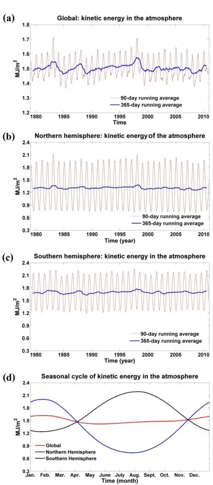
for the long-term variation of global kinetic energy are shown in Fig. 1. The inter-annual

103

variation of the total kinetic energy stock is associated with the changing phases of the El Ni o -

104

Southern Oscillation (ENSO) cycle (Fig. 1a and Fig. 2). During the warm El Nino phase (notably

105

years 1983, 1987, 1997 and 2010), elevated sea surface temperatures (SSTs) result in an increase

106

in the kinetic energy stock; during the cold phase La Nina phase (notably years 1985, 1989, 1999

107

and 2008), colder SSTs contribute to a decrease. The global kinetic energy stock averaged

108

approximately over the past 32 years, in the Northern Hemisphere

109

with in the Southern Hemisphere.

6

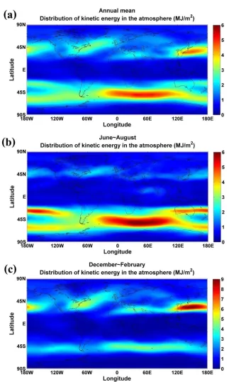
The spatial distributions of the annual mean, June - August, and December - February kinetic energy

111

budgets are shown in Fig. 3. Clearly evident is the influence of the dominant storm tracks at

mid-112

latitude, and the steady components of the subtropical and polar jet streams. There are two

113

distinct peaks in the Northern Hemispheric kinetic energy stock east of Japan and east of the

114

North American continent, with a more continuous belt of high kinetic energy located between

115

30 oS and 60 oS in the Southern Hemisphere. As discussed by Huang et al. [25], the boundary

116

layer wind, for example the wind at 100 m, is controlled by conditions in the free atmosphere,

117

perturbed by fast varying turbulence in the boundary layer. Strong winds in the free atmosphere

118

generally lead to strong winds near the surface, and consequently to high instantaneous values of

119

the capacity factors for wind turbines. The spatial distributions in Fig. 3 reflect the geographic

120

distribution and seasonality of wind resources as reported in the earlier studies [5, 26, 27].

121

4. Production of kinetic energy

122

For an air parcel of unit mass, production of kinetic energy may be written as:

123

124

where is the kinetic energy corresponding to unit mass, is the gravitational acceleration, is

125

the vertical velocity, is the velocity, is the air density, is the pressure and

126

force.

127

In calculating the kinetic energy production rate, it is convenient to consider the rate for

128

production of kinetic energy in a fixed unit of volume. Re-organizing equation (1), we have:

129

(2)

130

The left hand side of this equation denotes the rate per unit volume for production of kinetic

7

energy. The right hand side defines contributions to the production rate associated with the

132

convergence of the kinetic energy flux ( ), and the work carried out or consumed by

133

the pressure gradient force ( ), friction ( ) and gravity ( ).

134

The atmosphere is in quasi-hydrostatic balance: gravity is balanced approximately by the vertical

135

pressure gradient force. In this case, equation (2) may be recast in the simpler form:

136

(3)

137

where is the horizontal component of , and is the horizontal gradient of the pressure

138

force. Production of kinetic energy in the atmosphere, , can be estimated as

[17-139

22].

140

Fig. 4 illustrates the distribution of kinetic energy production, , averaged over the past 32 years

141

in units of . The tropical and subtropical region from 30 oS to 30 oN, dominated by

142

the thermally direct Hadley circulation, is responsible for a net source of kinetic energy as

143

indicated in Fig. 4a. The most prominent sources are located in the mid-latitude oceanic regions

144

below the pressure level, notably in the Southern Hemisphere, as depicted in Fig. 4c.

145

Production of kinetic energy in these regions is associated with the intense development of

146

eddies that stir the atmosphere over the ocean, carrying cold air equatorward and warm air

147

poleward, resulting consequently in cross-isobaric flow. The topographic forcing of the Tibetan

148

plateau has a noticeable impact on the production of kinetic energy in the upper region of the

149

atmosphere, from , as indicated in Fig. 4b.

150

The global and hemispheric rates for production of kinetic energy are obtained by integrating the

151

production term, , over the entire atmosphere or over each hemisphere separately. The global

152

kinetic energy production rate averaged over the past 3 decades is estimated at , with

8

a upward trend since the late 1990s (Fig. 5a). The average rate for production in the Northern

154

Hemisphere is , for the Southern Hemisphere. Hemispheric production

155

rates indicate strong seasonality (Fig. 5c), reaching maximum power output during local winter,

156

with minima in local summer.

157

5. Dissipation

158

Motions of the atmosphere against friction convert kinetic to internal energy. This process is

159

thermally irreversible, resulting in an increase in entropy. Approximately half of the frictional

160

dissipation takes place within the lowest kilometer of the atmosphere, a result of turbulent

161

motions generated mechanically by the flow over the underlying surface. The other half takes

162

place higher in the atmosphere where small-scale disturbances are generated as a result of

163

convection or shear instability of the vertical wind [28]. In the long run, the total kinetic energy

164

in the atmosphere, , is determined by a balance between production, , and dissipation by

165

friction, . The dissipation term may be quantified according to:

166

(4)

167

The long-term variation and seasonal cycle of are plotted in Fig. 6. Maximum dissipation

168

occurs in February, corresponding to the peak in Northern Hemisphere kinetic energy reflecting

169

the importance of surface roughness associated with Northern Hemisphere continental areas in

170

dissipating kinetic energy. The entropy generation associated with dissipation can be

171

approximated as

, where is the global average surface atmosphere (about ).

172

The fate of kinetic energy in the atmosphere from a mechanical perspective is summarized in Fig.

173

7. The residence time of kinetic energy, , calculated as , is 6.9 days.

174

6. The thermodynamics of atmospheric motions

9

According to the first law of thermodynamics:

176

(5)

177

where defines the rate per unit mass of dry air for diabatic heating, is the specific heat

178

of the air, is temperature, is the vertical component of wind velocity in an isobaric

179

system and [29].

180

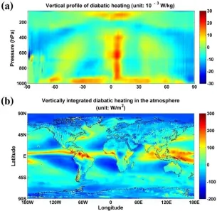
The annual mean spatial distribution of diabatic heating based on equation (5) is displayed in

181

Fig. 8. The results presented here are consistent with earlier studies [30, 31]. An important

182

fraction of the incoming sunlight reaches the surface which is heated accordingly. This heat finds

183

its way back into the atmosphere as a result of turbulent transport through the atmospheric

184

boundary layer. Most of the solar energy absorbed by the ocean is used to evaporate water. Water

185

vapor in the atmosphere acts as a reservoir for storage of heat that can be released later. As the air

186

ascends, it cools. When it becomes saturated, water vapor condenses with consequent release of

187

latent heat. Heating is dominated in the tropical atmosphere by release of latent heat. Separate

188

bands of relatively deep heating are observed at mid-latitudes where active weather systems

189

result in enhanced precipitation and release of latent heat.

190

The atmospheric system consists of dry air and water. Its total entropy and total static

191

energy , according to thermodynamics, can be expressed as: and

192

_{, where and represent the associated entropy and static energy of} 193

the dry air component and and represent the associated entropy and static energy of

194

the water component. The focus in this study is on how atmospheric motion of the dry air is

195

maintained by diabatic heating. Condensation and evaporation of water are treated accordingly

196

as external to the dry air component [32], namely as an exchange of entropy and energy with the

10

dry air.

198

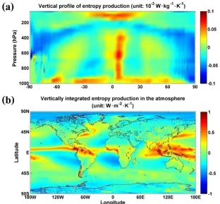
Regions of diabatic cooling, dominated by long wave radiation to space, occupy much of the

199

middle and upper troposphere. The rate of change of entropy, s, per unit mass is given by

200

. The spatial distribution of entropy generation is similar to the spatial pattern of , as 201

illustrated in Fig. 9.

202

Diabatic heating includes contributions from radiative heating and cooling, release of latent

203

heat associated with phase transitions, heating by conduction of sensible heat, and heating

204

by frictional dissipation:

205

(6)

206

where is the density of air, is the latent heat of condensation, and are the rates of

207

condensation and evaporation per unit mass, is the net radiative flux, is the sensible 208

heat flux due to conduction, is the wind tress tensor, and is the wind velocity.

209

The diabatic heating term can be written as , where accounts for

210

radiative heating (solar and infrared), latent heating and heating due to conduction:

211

(7)

212

The second component, , is associated with frictional dissipation:

213

(8)

214

By separating from , we may consider as the external heating responsible, from a

215

thermodynamic perspective, for the motion of the dry air. In the long run, the globally

216

integrated values for must be balanced by global production of kinetic energy, equal

217

therefore to . Consequently, we may rewrite the generation of entropy as:

11

(9)

219

where , and is the temperature of the environment in the region

220

where heat is either absorbed or released [33, 34].

221

In the long run, the entropy of the entire atmosphere must remain constant. Thus, with

222

the long term mean indicated by " ":

223

(10)

224

or

225

(11)

226

Since and are always positive, the second term representing the entropy

227

generation associated with dissipation is greater than zero, which implies that

228

. It follows that the and fields must be positively correlated. In 229

other words, the general circulation can be maintained against the disordering impact of

230

friction only if the heating occurs in warmer regions of the atmosphere with cooling in

231

colder regions. Fig. 10 summarizes the creation and dissipation of kinetic energy in the

232

atmosphere from a thermodynamic perspective.

233

The global heat source in Fig. 10 represents the heat that the atmosphere absorbs at the 234

higher temperature, , environment in order to do mechanical work. It is defined as

235

. The global heat sink in Fig. 10 represents the heat that the atmosphere 236

releases into the lower temperature, , environment and is defined by

237

12

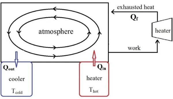
The mechanical work produced by the atmosphere is dissipated by friction and converted to heat

239

that is released back into the atmosphere. This process is thermally equivalent to using the

240

mechanical work to turn on a heater and return the exhausted heat back to the atmosphere, as

241

depicted in Fig. 10. However, it is difficult to distinguish between and , and the absolute

242

value of the global integral of is negligible compared to the global integral for and .

243

Thus, the global heat source can be approximated as: with

244

approximated as: .

245

The value for the global heat source averaged over the past three decades is estimated

246

at . The average kinetic energy production rate over the same period is calculated as

247

. It follows that the average efficiency for kinetic energy production is equal to

248

approximately .

249

The effective temperature at which heat is absorbed can be calculated as: 250

(12) 251

or approximated as:

252

(13) 253

where

, with and representing the starting and ending times for the 254

integration.In the long run, the entropy of the entire atmosphere is required to remain 255

constant. Equation (10) can be recast as:

256

(14)

257

where

represents the entropy generation due to dissipation [34]. The effective

13

temperature at which heat is released can be estimated accordingly.

259

The schematic illustration of the dry air component of the atmosphere as a thermal engine is

260

summarized in Fig. 11, with values included here representing averages for the past 32 years.

261

The dry air component of the atmosphere acts as a thermal engine, absorbing heat at a

262

temperature of approximately , releasing heat at a temperature of approximately .

263

The process produces kinetic energy at a rate of sustaining thus the circulation of the

264

atmosphere against friction.

265

7. Discussion and summary

266

The study started with a quantification of the total kinetic energy stock of the atmosphere and

267

subsequently investigated how kinetic energy is generated and dissipated from mechanical and

268

thermodynamic perspectives.

269

The total kinetic energy stock of the atmosphere displays significant inter-annual variability, as

270

indicated in Fig. 1 and Fig. 2, with the changing phases of the ENSO cycle playing an important

271

role. This inter-annual variation reflects the fact that the wind energy potential for a particular

272

location can fluctuate on a long-term basis, under the influences of long-term atmospheric

273

oscillations which can alter the circulation of the atmosphere including the distribution of kinetic

274

energy.

275

To illustrate the inter-annual variation of wind energy potentials, we select two locations, one in

276

Texas (34.5 oN, 101.3 oW) and the other in North Dakota (47 oN, 101.3 oW), as indicated in Fig

277

12a. In calculating the potential electricity generated from wind, we chose to use power curves

278

and technical parameters for the GE 2.5 MW turbines (rated wind speed 12.0 m/s, cut-in wind

279

speed 3.5 m/s, and cut-out speed 25.0 m/s). The power curve of the wind turbine defines the

14

variation of power output as a function of wind speed. The hourly wind speeds at 100 m are

281

extrapolated from winds at 50 m according to the relation:

, where V100

282

and V50 indicate hourly values for the wind speed at 100 m and 50 m respectively, Z100 and Z50 283

define the elevation of the turbine hub (100 m) and the reference 50 m altitude, and Z0 defines 284

the surface roughness length.

285

The capacity factor (CF) values in Fig. 12b, at a particular time , are calculated as:

286

(15) 287

where denotes the power actually realized, and refers to the power that could have

288

been realized had conditions permitted the turbine to operate at its name plate capacity. The

289

seasonality of wind energy potentials, represent by CF values, have been removed due to the

290

averaging period defined in equation (15): averaging from to .

291

CF values of the wind farms in Texas and North Dakota display significant interanual variation.

292

The ups and downs of CF values in Fig 12b are the embodiments of the long-term atmospheric

293

oscillations. Modern wind turbines are designed to work with an anticipated lifespan of 20 years.

294

Wind energy potentials, as exemplified by the Texas and North Dakota cases, can vary on a

year-295

to-year basis with a large amplitude over a 20 years period. Predictions of wind power for the

296

next 20 years, or at least limits on its possible variation, will pose an important challenge for

297

prospective investors in wind power.

298

The kinetic energy of wind in the atmosphere is constantly dissipated by friction. The residence

299

time of kinetic energy, , is estimated at 6.9 days. The dry air component of the atmosphere

300

generates kinetic energy as a thermal engine to sustain the general circulation of the atmosphere

15

against frictional dissipation. Key thermodynamic properties were quantified, including the

302

kinetic energy production rate, , the heat absorption rate, , the effective temperature at

303

which heat is absorbed, , and the effective temperature at which heat is released, .

304

The calculations of these key properties are based on the assimilated meteorological data from

305

the MERRA compilation. Data assimilation is the process of incorporating historical

306

observations of the atmosphere into a numerical physical model, and produces the most reliable

307

estimate of the past meteorological conditions. However, some uncertainties with the final

308

outputs, such as wind speed data, cannot be completely eliminated.

309

The kinetic energy production rate, , is calculated from a mechanical perspective using wind

310

speed data and pressure gradient data. Wind speed data and pressure data are accurately obtained

311

in the assimilation process [24]. Thus, the kinetic energy production quantified here is reliable,

312

and the results obtained are consistent with other studies [18-22]. The quantification of other

313

variables, notably diabatic heating and effective temperatures, involves parameters such as the

314

vertical velocity of the air with relatively large uncertainties [24]. Absolute values of these

315

thermodynamic properties are subject to relatively large uncertainty, depending as they do on the

316

accuracy of the input data, the MERRA analysis in the case. It is not possible to place error bars

317

on the values derived here for these parameters.

318

The globally averaged combined land and ocean surface temperature data indicate a warming of

319

0.85 K, over the period 1880 to 2012 [35]. A number of studies argued that the warming climate

320

over the past decades has influenced the wind resource potential [36-44]. The upward trend in

321

kinetic energy production rate obtained hereconfirms the fact that thethermodynamic conditions

322

of the atmosphere have undergone a significant change over the past 32 years. A key question is

16

whether the conclusions reached in the study may be conditioned by the use of a specific data

324

base. Other datasets including NCEP-1, NCEP-2, ERA-40 and JRA-25 should be employed in

325

future to compare with results from the present study. Regarding the future warming climate,

326

according to the IPCC 2014 report [35], the change in global surface temperature by the end of

327

the 21st century is likely to exceed 1.5°C relative to the average from year 1850 to 1900 under

328

most future greenhouse emission scenarios. It is essential to investigate how the atmosphere, as a

329

thermal engine, will adjust under the different scenarios, altering thus the distributions and values

330

of wind energy resources.

331

A number of studies have suggested that large scale deployment of wind farms could potentially

332

influence the circulation of the atmosphere [9, 11-16, 45-49]. With a simple parameterization of

333

turbine operations, Miller et al. [46] performed numerical experiments and found that a

334

maximum of of electricity could be generated. Marvel et al. [47] extended Miller's work

335

by parameterizing the turbines as sinks for momentum and concluded that wind turbines placed

336

at the Earth’s surface could extract kinetic energy at a rate of at least , whereas

high-337

altitude wind turbines could extract more than . With a different global model and

338

parameterization approach, Jacobson and Archer [48] argued that as the number of wind turbines

339

increases over large geographic regions, power extraction would first increase linearly, then

340

converge to a saturation limit, with a saturation potential in excess of at 100 m globally,

341

at 10 km. There is a notable discrepancy between these various estimates. Adams and

342

Keith [16] addressed the question using a mesoscale model. They concluded that wind power

343

production would be limited to about 1 W/m2 at wind farm scales larger than about 100 km2 and

344

that the mesoscale model results are quantitatively consistent with results from global models

345

that simulated the climate response to much larger wind power capacities. However, as noted

17

earlier, the energetics of the entire atmosphere is different from the energetics of the mesoscale

347

region.

348

The quantity of wind energy that can be extracted from the atmosphere to generate electricity

349

depends ultimately on the rate at which kinetic energy is produced, not on the quantity of kinetic

350

energy stored in the atmosphere [50]. Answering the question of the ultimate limit of the

351

atmosphere as a source of wind-generated electric power requires a detailed study of the

352

underlying thermodynamics of the global atmosphere. While not trying to quantify the ultimate

353

wind potential, this study provides an analytical framework that can be adapted for future studies

354

addressing the ultimate wind energy potential and the potential perturbations to the atmospheric

355

circulation that could arise as a result of significant exploitation of this potential. It will be

356

critical to understand how the key thermodynamic variables, such as the effective temperature

357

( and ) and diabatic heating ( and ), evolve as increasing numbers of large scale

358

wind farms are deployed.

359

360

Acknowledgements

361

The work described here was supported by the National Science Foundation, NSF-AGS-1019134.

362

Junling Huang was also supported by the Harvard Graduate Consortium on Energy and

363

Environment. We acknowledge helpful and constructive comments from Michael J. Aziz, and Xi

364

Lu.

18

Reference:

369

[1] The World Wind Energy Association 2013 report. April 2014, Bonn, Germany.

370

[2]Landberg L, Myllerup L, Rathmann O, Petersen EL, Jørgensen BH, Badger J, and Mortensen

371

NG. Wind resource estimation—an overview. Wind Energy 2003; 6:3-261.

372

[3] Hoogwijk M, de Vries B, and Turkenburg W. Assessment of the global and regional

373

geographical, technical and economic potential of onshore wind energy. Energy Economics 2004;

374

26:5-889.

375

[4] Archer CL, and Jacobson MZ. Evaluation of global wind power. Journal of Geophysical

376

Research: Atmospheres (1984–2012) 2005; 110:D12.

377

[5] Lu X, McElroy MB, and Kiviluoma J. Global potential for wind-generated electricity.

378

Proceedings of the National Academy of Sciences 2009; 106:27-10933.

379

[6] Tapiador FJ. Assessment of renewable energy potential through satellite data and numerical

380

models. Energy & Environmental Science 2009; 2:11-1142.

381

[7] de Castro C, Mediavilla M, Miguel LJ, and Frechoso F. Global wind power potential:

382

Physical and technological limits. Energy Policy 2011; 39:10-6677.

383

[8] Zhou Y, Luckow P, Smith SJ, and Clarke L. Evaluation of global onshore wind energy

384

potential and generation costs. Environmental science & technology 2012; 46:14-7857.

385

[9] Keith DW, DeCarolis JF, Denkenberger DC, Lenschow DH, Malyshev SL, Pacala S, and

386

Rasch PJ. The influence of large-scale wind power on global climate. Proceedings of the national

387

academy of sciences of the United States of America 2004; 101:46-16115.

19

[10] Wang C, Prinn RG. Potential climatic impacts and reliability of very large-scale wind farms.

389

Atmospheric Chemistry and Physics 2010; 10:4-2053.

390

[11] Wang C, Prinn RG. Potential climatic impacts and reliability of large-scale offshore wind

391

farms. Environmental Research Letters 2011; 6:2-025101.

392

[12] Walsh-Thomas JM, Cervone G, Agouris P, Manca G. Further evidence of impacts of

large-393

scale wind farms on land surface temperature. Renewable and Sustainable Energy Reviews, 2012;

394

16:8-6432.

395

[13] Fitch AC, Olson JB, Lundquist JK, Dudhia J, Gupta AK, Michalakes J, Barstad I. Local and

396

mesoscale impacts of wind farms as parameterized in a mesoscale NWP model. Monthly

397

Weather Review, 2012; 140:9-3017.

398

[14] Fitch AC, Lundquist JK, Olson JB. Mesoscale influences of wind farms throughout a

399

diurnal cycle. Monthly Weather Review 2013; 141:7-2173.

400

[15] Fitch AC, Olson JB, Lundquist JK. Parameterization of wind farms in climate models.

401

Journal of Climate 2013; 26:17-6439.

402

[16] Adams AS, Keith DW. Are global wind power resource estimates overstated?

403

Environmental Research Letters 2013; 8:1-015021.

404

[17] Lorenz EN. Available potential energy and the maintenance of the general circulation.

405

Tellus 1955; 7:2-157.

406

[18] Oort AH. On estimates of the atmospheric energy cycle. Monthly Weather Review 1964;

407

92:11-483.

20

[19] Oort AH, Yienger JJ. Observed interannual variability in the Hadley circulation and its

409

connection to ENSO. Journal of Climate 1996; 9:11-2751.

410

[20] Li L, Ingersoll AP, Jiang X, Feldman D, Yung YL. Lorenz energy cycle of the global

411

atmosphere based on reanalysis datasets. Geophysical Research Letters 2007; 34:16.

412

[21] Marques CAF, Rocha A, Corte-Real J. Comparative energetics of ERA-40, JRA-25 and

413

NCEP-R2 reanalysis, in the wave number domain. Dynamics of Atmospheres and Oceans 2010;

414

50:3-375.

415

[22] Kim YH, Kim MK. Examination of the global lorenz energy cycle using MERRA and

416

NCEP-reanalysis 2. Climate Dynamics 2013; 40:5-6.

417

[23] Lorenz EN. The nature and theory of the general circulation of the atmosphere (Vol. 218).

418

Geneva: World Meteorological Organization; 1967.

419

[24] Rienecker M, et al. The GEOS-5 data assimilation system—Documentation of versions

420

5.0.1 and 5.1.0. NASA GSFC, Tech. Rep. Series on Global Modeling and Data Assimilation

421

2007; NASA/TM-2007-104606, Vol. 27.

422

[25] Huang J, Lu X, McElroy MB. Meteorologically defined limits to reduction in the variability

423

of outputs from a coupled wind farm system in the Central US. Renewable Energy 2014; 62:

424

331-340.

425

[26] Heide D, Von Bremen L, Greiner M., Hoffmann C, Speckmann M, Bofinger S. Seasonal

426

optimal mix of wind and solar power in a future, highly renewable Europe. Renewable Energy

427

2010; 35:11-2483.

21

[27] Archer CL, and Jacobson MZ. Geographical and seasonal variability of the global “practical”

429

wind resources. Applied Geography 2013; 45: 119.

430

[28] Kung EC. Large-scale balance of kinetic energy in the atmosphere. Mon. Wea. Rev 1966;

431

94:11-627.

432

[29] Holton JR, and Hakim GJ. An introduction to dynamic meteorology. Academic press; 2013.

433

[30] Hagos S, et al. Estimates of tropical diabatic heating profiles: Commonalities and

434

uncertainties. Journal of Climate 2010; 23:3-542.

435

[31] Ling J, Zhang C. Diabatic heating profiles in recent global reanalyses. Journal of Climate

436

2013; 26:10-3307.

437

[32] Johnson DR. “General Coldness of Climate Models” and the Second Law: Implications for

438

Modeling the Earth System. Journal of climate 1997; 10:11-2826.

439

[33] Peixoto JP, Oort AH, De Almeida M, Tomé A. Entropy budget of the atmosphere. Journal

440

of Geophysical Research: Atmospheres (1984–2012) 1991; 96:D6-10981.

441

[34] Peixoto JP, Oort AH. Physics of climate. American institute of physics; 1992.

442

[35] Stocker TF, et al. Climate Change 2013. The Physical Science Basis. Working Group I

443

Contribution to the Fifth Assessment Report of the Intergovernmental Panel on Climate

Change-444

Abstract for decision-makers. Groupe d'experts intergouvernemental sur l'evolution du

445

climat/Intergovernmental Panel on Climate Change-IPCC, C/O World Meteorological

446

Organization, 7bis Avenue de la Paix, CP 2300 CH-1211 Geneva 2 (Switzerland), 2013.

447

[36] Breslow PB, Sailor DJ. Vulnerability of wind power resources to climate change in the

22

continental United States. Renewable Energy 2002; 27:4-585.

449

[37] Pryor SC, Schoof JT, Barthelmie RJ. Climate change impacts on wind speeds and wind

450

energy density in northern Europe: empirical downscaling of multiple AOGCMs. Climate Res.

451

2005; 29:183.

452

[38] Sailor DJ, Smith M, Hart M. Climate change implications for wind power resources in the

453

Northwest United States. Renewable Energy 2008; 33:11-2393.

454

[39] Bloom A, Kotroni V, Lagouvardos K. Climate change impact of wind energy availability in

455

the Eastern Mediterranean using the regional climate model PRECIS. Natural Hazards and Earth

456

System Science 2008; 8:6-1249.

457

[40] Pryor SC, Barthelmie RJ. Climate change impacts on wind energy: A review. Renewable

458

and sustainable energy reviews 2010; 14:1-430.

459

[41] Mideksa TK, Kallbekken S. The impact of climate change on the electricity market: A

460

review. Energy Policy 2010; 38:7-3579.

461

[42] Pereira de Lucena, AF, Szklo AS, Schaeffer R., Dutra RM. The vulnerability of wind power

462

to climate change in Brazil. Renewable Energy 2010; 35:5-904.

463

[43] Wan H, Wang XL, and Swail VR. Homogenization and trend analysis of Canadian

near-464

surface wind speeds. Journal of Climate 2010; 23:5-1209.

465

[44] Jiang Y, Luo Y, Zhao Z, Tao S. Changes in wind speed over China during 1956–2004.

466

Theoretical and Applied Climatology 2010; 99:3-4.

23

[45] Lu H, Porté-Agel F. Large-eddy simulation of a very large wind farm in a stable

468

atmospheric boundary layer. Physics of Fluids (1994-present) 2011; 23:6-065101.

469

[46] Miller LM, Gans F, Kleidon A. Estimating maximum global land surface wind power

470

extractability and associated climatic consequences. Earth Syst. Dynam 2011; 2:1-1.

471

[47] Marvel K, Kravitz B, Caldeira K. Geophysical limits to global wind power. Nature Climate

472

Change 2013; 3:2-118.

473

[48] Jacobson MZ, Archer CL. Saturation wind power potential and its implications for wind

474

energy. Proceedings of the National Academy of Sciences 2012; 109:39-15679.

475

[49] Roy SB, Traiteur JJ. Impacts of wind farms on surface air temperatures. Proceedings of the

476

National Academy of Sciences 2010; 107:42-17899.

477

[50] Gustavson MR. Limits to wind power utilization. Science 1979; 204:4388-13.

478

479

480

481

482

483

484

24

Figures

486

487

Fig. 1. (a) Variation of the global kinetic energy from January 1979 to December 2010. (b)

488

Variation of the Northern Hemisphere kinetic energy from January 1979 to December 2010. (c)

489

Variation of the Southern Hemisphere kinetic energy from January 1979 to December 2010. (d)

490

The composite seasonal cycle of the kinetic energy of the atmosphere averaged over the past 32

491

years.

25 494

495

496

Fig. 2. (a) The departure of global kinetic energy from its 32 years' mean value . The

497

seasonality of the departure is removed via 365-day running average. (b) The time series of the

498

multivariate ENSO index from January 1979 to December 2010. Positive values correspond to

499

the warm events of the ENSO phenomena, while the negative ones correspond to the cold events.

26 505

Fig. 3. (a) Spatial distribution of the annual mean kinetic energy of the atmosphere in ,

506

calculated based the past 32 years' data. (b) June ~ August, calculated based the past 32 years'

507

data. (c) December ~ February, based on the past 32 years' data.

27 510

Fig. 4. (a) The vertical profile of kinetic energy production rate, . (b) Kinetic energy production

511

rate, , in the layer between . (c) Kinetic energy production rate, , in the

512

layer between .

28 516

Fig. 5. (a) Variation of the global kinetic energy production rate, , from January 1979 to

517

December 2010. (b) Variation of the Northern Hemisphere kinetic energy production trend, ,

518

from January 1979 to December 2010. (c) Variation of the Southern Hemisphere kinetic energy

519

production trend, , from January 1979 to December 2010. (d) The composite seasonal cycle of

520

the kinetic energy production rate, , based on the past 32 years' data.

29 524

Fig. 6. (a) Variation of kinetic energy dissipation rate, , from January 1979 to December 2010;

525

(b) The composite seasonal cycle based on the past 32 years.

30 539

Fig. 7. Mechanical perspective on the budget of atmospheric kinetic energy.

31 551

Fig. 8. (a) Vertical profile of diabatic heating. (b) Vertically integrated results.

32 561

Fig. 9. (a) Vertical profile of entropy production. (b) Vertically integrated results.

33 571

Fig. 10. Schematic depiction of the atmosphere as a thermal engine.

34 588

Fig. 11. Illustration of the atmosphere as a Carnot engine. Work, , is dissipated ultimately by

589

friction.

590

591

592

593

594

595

596

597

598

35 600

Fig. 12. (a) Color coded values for CF as a function of position averaged over the 32 year period

601

Jan 1st 1979 to Dec 30th 2013. Positions of two wind farms considered in this paper are

602

indicated by the stars. (b) CF values for two wind farms in Texas and North Dakota with

603

seasonal cycle removed.