Measuring the spatial extent of texture pooling using reverse correlation

White Rose Research Online URL for this paper:

http://eprints.whiterose.ac.uk/103300/

Version: Accepted Version

Article:

Baker, Daniel Hart orcid.org/0000-0002-0161-443X and Meese, Tim S (2014) Measuring

the spatial extent of texture pooling using reverse correlation. Vision Research. pp. 52-58.

ISSN 0042-6989

https://doi.org/10.1016/j.visres.2014.02.004

[email protected] https://eprints.whiterose.ac.uk/ Reuse

This article is distributed under the terms of the Creative Commons Attribution (CC BY) licence. This licence allows you to distribute, remix, tweak, and build upon the work, even commercially, as long as you credit the authors for the original work. More information and the full terms of the licence here:

https://creativecommons.org/licenses/

Takedown

If you consider content in White Rose Research Online to be in breach of UK law, please notify us by

This post-print version was created for open access dissemination through institutional repositories.

Measuring the spatial extent of texture

pooling using reverse correlation

Daniel H. Baker

* & Tim S. Meese

1. Department of Psychology, University of York, Heslington, York, YO10 5DD, UK

2. School of Life & Health Sciences, Aston University, Birmingham, B4 7ET, UK

* email: [email protected]

Summary

The local image representation produced by early stages of visual analysis is uninformative regarding spatially extensive textures and surfaces. We know little about the cortical algorithm used to combine local information over space, and still less about the area over which it can operate. But such

operations are vital to support perception of real-world objects and scenes. Here, we deploy a novel reverse-correlation technique to measure the extent of spatial pooling for target regions of different areas placed either in the central visual field, or more peripherally. Stimuli were large arrays of micropatterns, with their contrasts perturbed individually on an interval-by-interval basis. By

comparing trial-by-trial observer responses with the predictions of computational models, we show that substantial regions (up to 13 carrier cycles) of a stimulus can be monitored in parallel by summing contrast over area. This summing strategy is very different from the more widely assumed signal selection strategy (a MAX operation), and suggests that neural mechanisms representing extensive visual textures can be recruited by attention. We also demonstrate that template resolution is much less precise in the parafovea than in the fovea, consistent with recent accounts of crowding.

Keywords:

reverse correlation; area summation; max operator

1 Introduction

The human visual system is structured hierarchically, with spatially local analyses at early stages feeding into representations of extensive textures, objects and surfaces at later stages. But despite extensive work focussing on local processes, e.g. in primary visual cortex (V1), we know relatively little about the later stages of representation. In particular, the limits of contrast integration across space, and the pooling strategy involved.

For several decades, the psychophysics

literature has favoured a probability

summation rule for pooling contrast beyond the classical receptive fields typically found in V1 (e.g. Mayer and Tyler, 1986; Robson and Graham, 1981) and contemporary accounts implement this with a MAX operator (Meese and Summers, 2012; Pelli, 1985; Tyler and Chen, 2000). This detection strategy is

sometimes referred to as signal selection

(Meese and Baker, 2011), since the MAX operator chooses one signal over several others.

An alternative strategy is signal combination,

in which many signals are combined to generate an overall response (Meese and Baker, 2011). In fact, a recent body of work supports

the signal combination account of spatial pooling over the signal selection account (Baker and Meese, 2011; Meese and Baker, 2011; Meese and Summers, 2012, 2007; Meese, 2010; Morgenstern and Elder, 2012). According to this work, the signal combination

strategy operates across various visual

dimensions such as space, time, orientation and eye (Meese and Baker, 2013). However, although several attempts have been made (Baker and Meese, 2011; Meese, 2010), it has been difficult to firmly establish the spatial extent of the signal combination process using conventional contrast detection techniques (Baker and Meese, 2011).

This post-print version was created for open access dissemination through institutional repositories.

observers in our study. Our analysis reveals that observers sum contrast over large areas (9-13 carrier cycles) using a signal combination strategy, rather than a signal selection (MAX) strategy, and that observers can be very poor at ignoring visual data at fixation, even when it is uninformative.

1.1 Simulated observers

We first consider the behaviour of two canonical model observers in a

two-interval-forced-choice (2IFC) contrast increment

detection task (see Materials & Methods): the Ôsumming observerÕ and the ÔMAXing

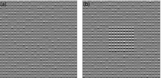
square region of the stimulus (e.g. Figure 1), with a width of 1, 3, 9 or 27 elements (defined by the white squares in Figure 2). On each trial, the summing observer adds the contrast values within the target region linearly, and selects the interval with the largest total as being the one most likely to contain the target. The MAXing observer selects the interval with the highest single contrast element in the target region. This process was repeated for 2000 trials per condition and observer. To mimic the non-determinacy of human observers, we added zero-mean Gaussian noise to the contrast of each element on every interval of every trial.

Figure 1: Example stimulus for null (a) and target (b) intervals of a contrast increment detection task. The contrast of each element was determined by a Gaussian distribution with a mean of 32% (i.e. it was a fixed contrast pedestal, with zero-mean noise added). In the target interval (b), a contrast increment was applied to elements in the target region, here a 9x9 element square in the centre of the display. In the experiments, the target increment was either 0% or near threshold, so was less salient than in the example above.

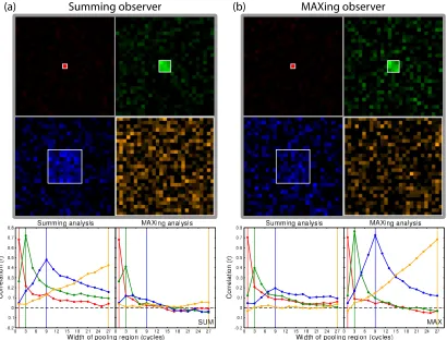
The behaviour of the model observers was analysed in two ways. First, we performed reverse correlation for each individual element on the contrast difference between the null and target interval and the interval selected by the observer. The correlation coefficients are plotted in Figure 2 (top row) as correlation maps, and are similar to classification images

(Ahumada, 2002). For both simulated

observers, correlations were concentrated in the target area for small target regions (red, green), and became more diffuse as targets grew larger (blue, orange). Using this technique, the two model observers produced similar maps, so there was no way to distinguish between the two very different decision rules.

A more informative analysis combines information across multiple elements, rather than treating each element independently. Pooling regions of different widths were

assessed, within which the sum or the MAX was correlated with the responses of the simulated observer. The strongest correlations occurred when the observer rule and the analysis rule matched (i.e. the. summing analysis, for the summing observer; the MAXing analysis, for the MAXing observer), and the pooling region equalled the target region, as shown by the graphs in Figure 2

(bottom row). When the rules were

mismatched, weaker correlations were

observed, particularly for the summing observer paired with the MAXing analysis. Thus, by applying this type of analysis to human results, we can determine which of the two pooling strategies they use, and also derive an estimate of the size of the stimulus region over which pooling takes place (which may be

sub-optimal owing to physiological

limitations). The results of this study have previously been reported in abstract form (Baker and Meese, 2013).

This post-print version was created for open access dissemination through institutional repositories.

Figure 2: Data from two model observers, who either summed (a) or MAXed (b) over the target region. The maps treat each element independently, and correlate the contrast difference across intervals with the observerÕs responses, over 2000 trials. Each map was peak-normalized, with the target regions indicated by white squares. Luminance at each location indicates how well the element there predicted responses, with correlations <=0 shown in black. In the lower graphs in each column, correlations were obtained by either summing or MAXing over a range of square windows to infer the width of the observerÕs pooling region and the decision rule used (see text).

2 Methods

2.1 Apparatus & Stimuli

All stimuli were presented on a gamma corrected NEC MultiSync Pro monitor running at 75Hz. Stimuli were generated in Matlab running on an Apple computer, and presented at 14-bit greyscale resolution by a BITS++ box (Cambridge Research Systems, Kent, UK). The monitor was viewed from 91cm, such that 48 monitor pixels subtended one degree of visual angle. Throughout, we define contrast as

Michelson contrast in percent (C% = (Lmax

-Lmin)/(Lmax+Lmin), where L is luminance), often

expressed in decibels (CdB = 20log10(C%)).

Stimuli were square arrays of 27x27

ÔBattenbergÕ micropatterns (see Meese, 2010) with a spatial frequency of 2c/deg. In brief, these are constructed from a horizontal sinusoidal grating, which is contrast modulated by a full-wave rectified vertical sinusoidal grating at half the carrier spatial frequency. This segments the stimulus into vertical columns of horizontal stripes. Horizontal

segmentation occurs naturally at the zero crossings of the carrier grating, and is accentuated by the contrast differences between the elements (carrier cycles). The contrast of each element was sampled independently on each interval of every trial from a Gaussian distribution (in linear contrast units) with a standard deviation of 10% (20dB), and a mean of 32% (30dB) (this is equivalent to a pedestal of 30dB with contrast jitter (Ò0D noiseÓ, see Baker and Meese, 2012) added). Example stimuli are shown in Figure 1. On the very rare occasions (<0.15% of elements) when an elementÕs contrast exceeded 100% or fell below 0% they were fixed at these limiting values.

2.2 Procedures

Observers viewed the display from a head-and-chin rest. The task was a two interval forced choice (2IFC) contrast increment detection between two noisy Battenberg textures (see above). One interval contained the target, the other did not, and they were presented in random order for 100ms (with an interstimulus

Summing observer

MAXing observer

This post-print version was created for open access dissemination through institutional repositories.

indicate using the buttons of a computer

trackball which interval they believed

contained the target. Before beginning the main experiments, we used a staircase procedure to estimate increment thresholds for the various conditions. The thresholds from this procedure guided our choice of contrasts used in the main experiments. No feedback was given in any experiment.

In Experiment I there were four target sizes, all of which were square, with widths of 1, 3, 9 and 27 elements. The target regions were centrally located. Observers were explicitly informed of target spatial extent by a quad of continuously present dark dots that framed the target area. For each target array size, observers completed 20 blocks of 100 trials using the method of constant stimuli. There were two target contrast levels: 0% and a near-threshold level informed by the staircase procedure described above. For all observers, these near-threshold contrasts were 22dB (12.6%) for the 1x1 target, and 12dB (4%) for the other target sizes. We included the non-zero target contrast to keep observers on task, and the 0% contrast because this produces data that is uncontaminated by the presence of a physical target (e.g. the observer is comparing two statistically identical noise fields in each trial). The blocks for different target sizes were run separately in a random order, and each block lasted around 3 minutes. Each observer completed 2000 trials for each target size, split between the two target contrast levels.

In Experiment II there were two conditions. In the first, a one-element target was offset below fixation by three elements. In the second, there were two target locations, equidistant above and below fixation; the target appeared in both locations in every trial. Quads of dark dots indicated the locations of the target and fixation elements. The target contrast levels were 0% and either 20% (26dB; DHB & SAW) or 32% (30dB; TSM), based on pilot staircase data. These pilot data can be considered to be practice sessions, with observers completing around 160 trials for each target size and location.

We calculated correlations between the observer responses and the contrast difference across intervals for each trial. To avoid bias, the target contrast increments were not included in the calculation of contrast difference between the null and target intervals. Positive differences indicate a higher contrast in the target interval and, on average, should

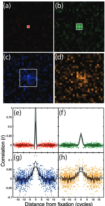
Figure 3: Correlation maps (a-d) and cross-section traces (e-h) for observer DHB for four target sizes (indicated by the white squares in panels a-d). The maps (a-d) are normalized to the maximum value for each map, with correlation coefficients <=0 shown as black. The trace plots (e-h) show absolute values (note the different scales for the ordinate across the rows). Coloured points are correlation values for individual elements, plotted as a function of absolute distance from the central fixation element (and mirrored about zero). The black trace is the average of the individual correlations at each location, and the grey curves are fitted Gaussian functions with two free parameters.

correspond to ÔcorrectÕ observer responses. Because the response data are binary, and the

contrast differences continuous, the

appropriate statistic is the point biserial correlation. This has an effective maximum

limit of r≈0.8, because the binary response

data can never fully predict the continuous contrast difference data. The calculations were performed on an element-by-element basis to produce the correlation maps in Figures 2 & 3, and on the sum or MAX over groups of elements for the more elaborate analysis (e.g. Figure 4). We initially calculated correlations for the two target contrast levels separately but, since these produced very similar results, we

0 0.25 0.5 0.75 1 Correlation (r)

-15 -10 -5 0 5 10 15

Distance from fixation (cycles)

-0.1 -0.05 0 0.05 0.1

-15 -10 -5 0 5 10 15 0 0 0.25 0.25 0.5 0.5 0.75 0.75 1 1 Correlation (r ) Correlation (r) -15

-15 -10-10 -5-5 00 55 1010 1515

Distance from fixation (cycles) Distance from fixation (cycles)

-0.1 -0.1 -0.05 -0.05 0 0 0.05 0.05 0.1 0.1 -15

-15 -10-10 -5-5 00 55 1010 1515

(e)

(a)

(b)

(c)

(d)

(f )

This post-print version was created for open access dissemination through institutional repositories.

pooled the data across contrast levels to give us 2000 trials per correlation.

2.3 Observers

Three observers completed all conditions. These were the two authors (DHB, TSM), and a psychophysically experienced postdoctoral researcher (SAW) who was na•ve regarding the specific expectations of the study. All observers had normal or corrected-to-normal visual acuity

3 Results

3.1 Experiment I: monitoring targets of different sizes

Example correlation maps for a representative human observer (DHB) are shown in Figure 3a-d, with fits to the data in Figure 3e-h. For

the small target regions (red, green),

correlations were strong in the expected locations, and weak outside of them, just as for the simulated observers (Figure 2). However, for the two larger target regions (blue, orange) there was a clear clustering of correlation coefficients in the centre of the stimulus. This suggests that contrast integration occurs over a limited range, and is non-uniform over space.

To uncover the decision rule used by human

observers, we calculated correlation

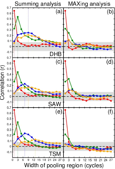
coefficients for all three observers for each of several pooling windows (various widths) and the two decision rules described above. As shown in Figure 4, correlations were stronger for the summing rule (left panels) than the MAXing rule (right panels) in all cases. This

indicates the existence of summing

mechanisms that are either pre-wired (in size),

or constructed according to prevailing

demands. It argues against peak-picking (akin to probability summation) from a population of local mechanisms.

Next we asked how spatially extensive the pooling is. We estimated this from the location of the peak in the correlation functions (Figure 4a,c,e) for each observer for each stimulus size. For the smaller target sizes (red, green), the correlations peak at windows of 1 and 3 cycles wide, as for the model observers (Figure 2), suggesting that the human observers selected a pooling region matched to the size of the stimulus in these two conditions. For the 9x9 element region (blue), one observer (DHB) appears to have monitored the full target region, whereas the other two (SAW, TSM) monitored a slightly smaller region, 7 elements

wide. For the largest target, observers DHB and SAW based their responses only on the central 9x9 elements, whereas TSM was able to sum over 13x13 elements. However, none of the three observers could uniformly monitor the entire 27x27 element region. Also, note that the correlation functions for the largest target are much less sharply peaked than those for smaller regions or for the model observers (Figure 2). This might derive from trial-to-trial variability in the size of the pooling regions that observers used, perhaps caused by switching across pooling mechanisms of different sizes and positions, or perhaps variations in fixation or attention.

Figure 4: Correlation coefficients for 3 observers, calculated for different pooling widths monitored by the model observer using either a summing (a,c,e) or MAXing (b,d,f) rule. Dotted lines indicate the location of the peak of each function for the summing analysis. The grey shaded region indicates the range of r values that are not significant at

p<0.05 for 2000 observations (Bonferroni corrected for 336 multiple comparisons (14 widths * 4 target sizes * 2 analysis methods * 3 observers)). Points outside of the shaded region indicate statistically significant correlations.

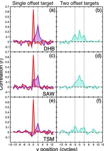
3.2 Experiment II: monitoring targets away from fixation

This post-print version was created for open access dissemination through institutional repositories.

(purple), or a pair of elements offset above and below fixation by the same amount (turquoise). For comparison, the equivalent function from the first experiment for a single central target element is shown in red. We confirmed that there were no significant correlations for the elements in adjacent horizontal locations, and so plot correlations only for the vertical column of elements within which the target(s) were placed.

Figure 5: Correlations between element state and observer response for targets at fixation (red) or displaced from fixation (purple, turquoise). Dotted lines indicate the target locations for the displaced conditions. It is clear that inappropriate pooling occurred when the target was away from fixation. Some observers (DHB, SAW) even produced stronger correlations at (e.g. based more of their decisions on) the fixated element than at the target elements (panels b & d).

For a single displaced element (purple), all observers produced maximum correlations at the target location (dotted line). However, whereas for a centrally placed element (red) the adjacent elements showed no (or

sometimes negative) correlation with

performance, pooling occurred over a larger area for a peripheral element (purple). For observer DHB, this broader spatial footprint is approximately symmetrical about the target element. For SAW there is a hint of an additional peak at the fixated location, whereas TSM shows an inhibitory trough at fixation, and at the adjacent element on the far side to the target. These individual differences might

uncertainty, between observers.

When targets were placed on both sides of fixation, there was even greater variation between observers. TSM shows a bimodal function (Figure 5f), though the correlations are weak (~0.1), and more widely distributed in space (turquoise) than for a single central element (red). DHB showed a similar pattern with stronger correlations, but also showed substantial contribution from the central fixated location, even though this element was uninformative for the task (Figure 5b). Observer SAW (Figure 5d) based his responses on a broad region centred on the fixation point, with by far the strongest correlations occurring at and around the uninformative element at fixation.

These variations in peripheral strategy are surprising, and might suggest that some observers are very poor at dividing their attention consistently across two spatial locations, or at suppressing the influence from uninformative locations. Alternatively, it may be that small or spatially localised detectors are not available in the periphery, and responses are based on mechanisms that pool over a larger region of space (e.g. for SAW). We note that all observers were able to perform the detection task effectively, achieving 75% (DHB), 67% (SAW) and 79% (TSM) correct in the target-present trials. However, as detailed in the Methods section, observer TSM required a factor of 1.58 (4dB) more target contrast relative to the other two observers to achieve this level of performance.

4 Discussion

We used a reverse correlation technique to estimate the maximum area over which

observers can combine contrast, and

demonstrated that this occurs by summing linearly over space, rather than merely selecting the region of highest contrast response. We also show that contrast increment detection becomes markedly less spatially precise when dissociated from fixation, and that some observers are unable to ignore an uninformative region around the

fixation point. We now discuss the

This post-print version was created for open access dissemination through institutional repositories. 4.1 Area summation of contrast involves signal

combination

A long-standing account (Robson and Graham, 1981) of the increase in contrast sensitivity with stimulus area (area summation) is that the

improvement in performance owes to

probability summation over multiple

independent, spatially localised detectors (see Tyler and Chen, 2000; Meese & Summers, 2012). An alternative explanation supposes that local detectors are summed at a later stage of processing producing mechanisms with a spatially extensive footprint (see Baker and Meese, 2011; Meese and Summers, 2007, 2012; Meese, 2010; Morgenstern and Elder, 2012). We have compared the predictions of these two models in several studies of contrast sensitivity (e.g. Baker and Meese, 2011; Meese and Summers, 2012, 2007; Meese, 2010; Morgenstern and Elder, 2012), all of which have favoured the linear summation account. The results here provide strong evidence that this signal combination strategy also predicts observer responses on a trial-by-trial basis better than a signal-selection (MAXing) strategy (see also Morgenstern and Elder, 2012). This result does not necessarily exclude the possibility that observers can use a MAXing strategy when it is appropriate for the task. In paradigms such as visual search, this may very well be the preferred option. However, our results indicate that pooling mechanisms that sum contrast are available to perception, and can be used in this type of experiment.

Previous estimates of the largest available size of pooling region have largely come from

detailed computational modelling of

psychophysical detection data. Meese & Summers (2007) concluded that their observers must have been pooling over at least 7 cycles of the carrier grating to produce the observed levels of empirical area summation. Meese (2010) cautiously extended this estimate to 16 cycles using so-called Battenberg stimuli. Using stimuli similar to Meese and Summers (2007), but a wider range of spatial frequencies, Baker & Meese (2011) estimated pooling regions of more than 12 carrier cycles.

The present results permit a more direct

estimate of maximum pooling widths.

Assuming a square integration region, our observers behaved in a way consistent with pooling over widths of up to 9 (DHB, SAW) or 13 (TSM) cycles (Figure 4) for the largest stimuli. We obtained further estimates by fitting isotropic 2D Gaussian functions to the

correlation maps (see Figure 3e-h). For the largest target size, best fitting functions indicate pooling over a full-width-at-half-height (2.35*SD) of between 7 (DHB, SAW) and 11.4 (TSM) grating cycles, broadly consistent with the estimates assuming a hard-edged square summation field.

Thus, overall, two very different approaches (our previous studies above, and the one here) both lead to the conclusion that summation can extend over a substantial portion of the stimulus when the task requires it. Furthermore, we note also that the individual differences between DHB, SAW and TSM are similar across the two studies in which these three observers took part. In Baker and Meese (Baker and Meese, 2011) and here, TSM summed over a larger region than did DHB and SAW. This is also consistent with other informal observations in our laboratory. What remains less clear is why observers are unable to extend the summation field even further so as to improve performance for the larger stimuli.

4.2 Is pooling the same as attention?

In our experiments, observers monitored a large array of elements, and were instructed to base their responses on some subset of those elements. In 50% of trials, no contrast increment was applied to the elements designated as ÔtargetÕ, so the only difference in behaviour was due to the instructions. Thus, observers can deploy their spatial attention according to instructions. This could involve attending to multiple V1-type mechanisms spread across the stimulus and summing their

responses (i.e. constructing a pooling

mechanism by demand), or attending to an

appropriately sized pre-wired pooling

mechanism. So what implications might this have for our understanding of spatial attention? The widespread notion of an attention ÔbeamÕ that can be directed around a stimulus at will comes largely from work on visual search (reviewed in Carrasco, 2011) and is usually

conceptualised as monitoring local

mechanisms at multiple spatial locations. But as suggested above, if a range of different sized pooling mechanisms were available to the observer, one can conceive of attention as deploying the mechanism most appropriate to the task, e.g. a single large mechanism to monitor a wide area. In other words, the ÔbeamÕ becomes ÔdefocussedÕ for large stimuli, rather than moving around in space. Our observation that peripheral stimuli are poorly resolved

This post-print version was created for open access dissemination through institutional repositories.

with poorer peripheral resolution (Baldwin et al., 2012), increased positional uncertainty (Levi et al., 1987; Michel and Geisler, 2011), or some explanations of crowding phenomena (e.g. Parkes et al., 2001). The variation in observersÕ success in dividing their attention

between two locations (and ignoring

intermediate ones) is consistent with the lack of consensus on human ability to do this successfully (Jans et al., 2010). However, it could be that with training and/or feedback, observers might improve at this task.

Throughout, we have discussed the width of pooling (or attention) in terms of cycles of the carrier grating. Although here we used only a single spatial frequency, our previous work (Baker and Meese, 2011) has indicated that area summation could be invariant of the carrier frequency when expressed in terms of cycles (see also Howell and Hess, 1978), as is also the case for retinal inhomogeneity (Baldwin et al., 2012; Pointer and Hess, 1989; Robson and Graham, 1981). Since natural scenes are broadband (Field, 1987), predicting which combination of mechanisms will govern performance in everyday environments is not straightforward. We anticipate that advances in this area will require combining multiscale filter models (e.g. Georgeson et al., 2007) with detailed formal models of attention (e.g. Gobell et al., 2004).

4.3 Comparison with classification image (CI) studies

The reverse correlation technique used here to produce the correlation maps (e.g. Figure 3) is related to the CI technique (Ahumada, 2002; Morgenstern and Elder, 2012; Murray, 2011). We also calculated CIs for our experiment by averaging the contrasts of the intervals selected by the observers as containing the target, and subtracting the averaged contrasts from the other (nonselected) intervals. When

peak-normalized, these were almost

indistinguishable from our correlation maps (i.e. Figure 3), revealing a close similarity between the two methods (not shown). However, calculating correlation coefficients is more flexible, as it can be easily extended to compare different models and decision rules, as we have done (e.g. Figure 4).

We think that our approach here is valuable for two reasons. First, our use of contrast jitter instead of white pixel noise means that larger templates can be measured without using extremely large pixel sizes (or requiring

sizes). Second, the testing of model hypotheses on a trial-by-trial basis is very powerful (see also Morgenstern and Elder, 2012; Neri, 2011), and offers important insights beyond the visual representation of the observerÕs template produced by standard CI techniques (reviewed in Murray, 2011). We note that a recent study (Morgenstern and Elder, 2012) also used a classification image method to ask related questions about spatial pooling strategies. This work, which used traditional white pixel noise, also found evidence for signal combination over signal selection, and provided estimates of the local filters used for detection, but did not attempt to estimate of the size of the pooling region.

5 Conclusions

We have presented a new multivariate technique for measuring the extent of spatial

pooling. Reverse-correlation shows that

pooling extends to around 9-13 carrier cycles, and can be precisely limited to small target areas in the central visual field. However, spatial precision is much poorer for larger stimuli, and for small stimuli placed in the

parafovea. These findings prompt new

metaphors for spatial attention, and indicate

that large aggregating mechanisms are

available to top-down monitoring in basic detection tasks.

6 Acknowledgements

Supported by EPSRC Grant EP/H000038/1.

7 References

Ahumada, A.J., 2002. Classification image

weights and internal noise level

estimation. J Vis 2, 121Ð31.

Baker, D.H., Meese, T.S., 2011. Contrast integration over area is extensive: a three-stage model of spatial summation. J Vis 11, (14): art. 14, 1-16.

Baker, D.H., Meese, T.S., 2012. Zero-dimensional noise: the best mask you never saw. J Vis 12(10): art. 20, 1-12. Baker, D.H., Meese, T.S., 2013. Using

psychophysical reverse correlation to measure the extent of spatial pooling of luminance contrast. Perception 41, 1512. Baldwin, A.S., Meese, T.S., Baker, D.H., 2012.

This post-print version was created for open access dissemination through institutional repositories.

within the central visual field. J. Vis. 12(11): art. 23, 1-17.

Carrasco, M., 2011. Visual attention: The past 25 years. Vision Res. 51, 1484Ð1525. Field, D.J., 1987. Relations between the

statistics of natural images and the response properties of cortical cells. J Opt Soc Am A 4, 2379Ð94.

Georgeson, M.A., May, K.A., Freeman, T.C.A., Hesse, G.S., 2007. From filters to features: Scale-space analysis of edge and blur coding in human vision. J. Vis. 7(13): art. 7, 1-21.

Gobell, J.L., Tseng, C., Sperling, G., 2004. The spatial distribution of visual attention. Vis. Res 44, 1273Ð96.

Howell, E.R., Hess, R.F., 1978. The functional area for summation to threshold for sinusoidal gratings. Vision Res. 18, 369Ð 374.

Jans, B., Peters, J.C., De Weerd, P., 2010. Visual spatial attention to multiple locations at once: the jury is still out. Psychol Rev 117, 637Ð84.

Levi, D.M., Klein, S.A., Yap, Y.L., 1987. Positional uncertainty in peripheral and amblyopic vision. Vision Res. 27, 581Ð 597.

Mayer, M.J., Tyler, C.W., 1986. Invariance of the slope of the psychometric function with spatial summation. J Opt Soc Am A 3, 1166Ð72.

Meese, T.S., 2010. Spatially extensive

summation of contrast energy is revealed by contrast detection of micro-pattern textures. J Vis 10(8): art. 14, 1Ð21. Meese, T.S., Baker, D.H., 2011. Contrast

summation across eyes and space is revealed along the entire dipper function by a ÒSwiss cheeseÓ stimulus. J Vis 11(1): art. 23, 1-23.

Meese, T.S., Baker, D.H., 2013. A common rule for integration and suppression of luminance contrast across eyes, space, time, and pattern. i-Perception, 4, 1Ð16.

Meese, T.S., Summers, R.J., 2007. Area summation in human vision at and above detection threshold. Proc R Soc Lond B Biol Sci 274, 2891Ð900.

Meese, T.S., Summers, R.J., 2012. Theory and data for area summation of contrast with and without uncertainty: Evidence for a noisy energy model. J Vis 12(11): art. 9, 1-28.

Michel, M., Geisler, W.S., 2011. Intrinsic position uncertainty explains detection

and localization performance in

peripheral vision. J. Vis. 11(1): art. 18, 1-18.

Morgenstern, Y., Elder, J.H., 2012. Local Visual Energy Mechanisms Revealed by Detection of Global Patterns. J. Neurosci. 32, 3679Ð3696.

Murray, R.F., 2011. Classification images: A review. J Vis 11(5): art. 2, 1-25.

Neri, P., 2011. Coarse to fine dynamics of monocular and binocular processing in human pattern vision. Proc Natl Acad Sci USA 108, 10726Ð31.

Parkes, L., Lund, J., Angelucci, A., Solomon, J.A., Morgan, M., 2001. Compulsory averaging of crowded orientation signals in human vision. Nat Neurosci 4, 739Ð44. Pelli, D.G., 1985. Uncertainty explains many aspects of visual contrast detection and discrimination. J Opt Soc Am A 2, 1508Ð 32.

Pointer, J.S., Hess, R.F., 1989. The contrast sensitivity gradient across the human visual field: with emphasis on the low spatial frequency range. Vision Res. 29, 1133Ð1151.

Robson, J.G., Graham, N., 1981. Probability summation and regional variation in contrast sensitivity across the visual field. Vis. Res 21, 409Ð18.

Tyler, C.W., Chen, C.C., 2000. Signal detection theory in the 2AFC paradigm:

attention, channel uncertainty and