Identifying road user classes based on repeated trip behaviour using Bluetooth data

Contents lists available atScienceDirect

Transportation Research Part A

journal homepage:www.elsevier.com/locate/tra

Identifying road user classes based on repeated trip behaviour

using Bluetooth data

F. Crawford

, D.P. Watling

, R.D. Connors

A R T I C L E I N F O

Keywords:

Intrapersonal variability Bluetooth data Sequence alignment Model based clustering

A B S T R A C T

Analysing the repeated trip behaviour of travellers, including trip frequency and intrapersonal variability, can provide insights into traveller needs,flexibility and knowledge of the network, as well as inputs for models including learning and/or behaviour change. Data from emerging data sources provide new opportunities to examine repeated trip making on the road network. Point-to-point sensor data, for example from Bluetooth detectors, is collected usingfixed detectors installed next to roads which can record unique identifiers of passing vehicles or travellers which can then be matched across space and time. Such data is used in this research to segment road users based on their repeated trip making behaviour, as has been done in public transportation research using smart card data to understand different categories of users. Rather than deciding on traveller segmentation based on a priori assumptions, the method provides a data driven approach to cluster together travellers who have similar trip regularity and variability between days. Measures which account for the strengths and weaknesses of point-to-point sensor data are presented for (a) spatial variability, using Sequence Alignment, and (b) time of day variability, using Model Based Clustering. The proposed method is also applied to one year of data from 23

fixed Bluetooth detectors in a town in northwest England. The data consists of almost 7.5 million trips made by over 300,000 travellers. Applying the proposed methods allows three traveller user classes to be identified: infrequent, frequent, and very frequent. Interestingly, the spatial and time of day variability characteristics of each user class are distinct and arenotlinearly correlated with trip frequency. The frequent travellers are observed 1–5 times per week on average and make up 57% of the trips recorded during the year. Focusing on these frequent travellers, it is shown that these can be further separated into those with high spatial and time of day variability and those with low spatial and time of day variability. Understanding the distribution of tra-vellers and trips across these user classes, as well as the repeated trip characteristics of each user class, can inform further data collection and the development of policies targeting the needs of specific travellers.

1. Introduction

While considering daily snapshots of transport networks is sufficient for many purposes, the benefits of considering the patterns and variability in each individual’s behaviour over days, months and even years is receiving increasing research attention. It can inform us about traveller habits (Minnen et al., 2015), predictable differences in travel patterns (Cherchi et al., 2017) and traveller

https://doi.org/10.1016/j.tra.2018.03.027

Received 5 April 2017; Received in revised form 21 January 2018; Accepted 25 March 2018

⁎_{Corresponding author.}

E-mail address:fi[email protected](F. Crawford).

flexibility (Kitamura et al., 2006), all of which are important for developing new policies and modelling travellerresponseto those policies, for example using day-to-day dynamical models which include micro-level learning mechanisms (Chen and Mahmassani, 2004; Liu et al., 2006). Understanding the current behaviour of travellers, not just on a single day but over days, weeks and months, also provides information about traveller needs and knowledge of the network.

A common assumption is that urban traffic, particularly the morning peak, consists of commuters who drive between home and work at the same time each weekday. This assumption is often made implicitly and largely for convenience but is rarely challenged despite increases in part time,flexible and home working in recent years. In Great Britain, a 2013 survey (Department for Business, Innovation and Skills, 2014) found that 80% of workplaces with at least 5 employees had part time staff, and other forms offlexible working such as reduced hours,flexitime and compressed hours had all increased since thefirst comparable survey in 2000. As-sumptions about the regularity of travellers is likely to influence the types of policies formulated to reduce morning peak congestion, some of which may perform differently based on the repeated trip making behaviour of travellers. For example, if the proportion of frequent travellers is overestimated, then the benefits to travellers of switching to public transportation due to savings from weekly or monthly tickets would also be overestimated. Similarly, making an assumption that all travellers have very little departure time flexibility would underestimate the impact of interventions such as time of day specific congestion charging.

One of the reasons why behaviour over multiple days is often overlooked may be the difficulty in collecting data. Detailed information about repeated trip making behaviour has typically been collected using multi-day travel diaries (Muthyalagari et al., 2001; Schlich and Axhausen, 2003; Elango et al., 2007). Such surveys provide data of great depth, but at a cost–bothfinancially and in terms of respondent burden. For example, the National Travel Survey in England involves face to face interviews and 7 day travel diaries for individuals in 7000 households and costs approximately £2.1 million per year to collect and process (Data.gov.uk, 2012). Respondent burden can be decreased by using GPS devices to track participants (Muthyalagari et al., 2001), but costs remain high, resulting in surveys which often are for short periods of time and/or have small sample sizes. For example, the 7 day travel diaries undertaken annually in England have a relatively large sample size, but sample sizes are usually much smaller for longer surveys, for example the six week Mobidrivesurvey collected in 1999 in Karlsruhe and Halle in Germany had 317 participants in 139 households (Axhausen et al., 2002).

More recently, emerging data sources have been explored to determine their usefulness with respect to measuring repeated trip making behaviour. Mobile phone data has been used to examine activity spaces, as inJärv et al. (2014), but the spatial precision is relatively low. In public transportation research, the availability of smart card data has resulted in researchers identifying different types of user based on their travel behaviour over time (Chu and Chapleau, 2010; Kieu et al., 2015; Goulet Langlois et al., 2016). Goulet Langlois et al. (2016)analysed four weeks of smart card data from London and identified four types of regular commuter. The daily and weekly activity sequences constructed using the smart card data had distinct patterns for each of these four groups:‘typical’ commuters, commuters who sometimes did not take public transportation home at night, commuters who used public transport as their main mode at the weekend and commuters who travelled less during school holiday periods.

The current paper examines data which could be considered the road network counterpart to smart card data, namely point-to-point sensor data, which includes Bluetooth and Automatic Number Plate Recognition (ANPR) data. Point-to-point-to-point‘sensors’ or

‘detectors’collect unique identifiers, either for vehicles or travellers, at fixed locations. It is this“re-identification and tracking”

ability which defines this type of data (Antoniou et al., 2011, p140) and as the unique identifiers can be matched over space and time, the data is ideal for examining repeated trip making. Where point-to-point sensors are permanently installed, the amount of data collected can quickly become very large. For example, in Section3an application to one year of data from 23 detectors is presented, and that data contains almost 7.5 million trips. These trips are obtained from processing 29.7 million observations, each of which corresponds to a Bluetooth device passing a detector.

Analysing such data with respect to repeated trip behaviour as a whole is not straightforward, however. Previous research on repeated trip making has usually focused on a single aspect, for example trip frequency (Elango et al., 2007; Tarigan and Kitamura, 2009), spatial variability (Buliung et al., 2008; Järv et al., 2014), time of day variability (Kitamura et al., 2006; Chikaraishi et al., 2009) or mode choice (Cherchi and Cirillo, 2014; Heinen and Chatterjee, 2015). Other research has combined different aspects to create a single measure of intrapersonal variability (seeSchlich and Axhausen (2003)for an overview). Calculating a single Similarity Index for travellers can be limiting, however, as it cannot account for travellers which differ in terms of different aspects of varia-bility, for example travellers whose trips are spatially predictable but unpredictable in terms of the time of day at which they occur. The current paper uses cluster analysis to segment travellers based on measures relating to multiple aspects of intrapersonal variability, as has been done for public transport users (Goulet Langlois et al., 2016). The methods proposed to measure the different aspects are distinctive from previous work, however, due to the nature of the data available from point-to-point sensors. Firstly, point-to-point sensor data does not generally provide origin or destination information due to limited network coverage and the possibility that many trips start and/or end outside the monitored area. It does not provide information about trip purpose either. This means that existing approaches for measuring spatial variability are not suitable. Existing approaches include measuring the distance travelled from home (Bayarma et al., 2007) and comparing daily activity sequences (Goulet Langlois et al., 2016). Secondly, point-to-point sensor data can provide some route choice information, depending on sensor locations, and it would be preferable to have a methodology which takes this additional information into account. Thirdly, for time of day variability, adjustments need to be made since the observations are not departure times.

data. The methodology could be applied to any type of point-to-point sensor data, but Bluetooth is probably the most relevant currently due to its increasing popularity for measuring travel times on the road network. It is a data driven approach which clusters together travellers who have similar trip regularity and variability between days without relying on a priori assumptions. The proposed methodology includes using Sequence Alignment to examine spatial variability and Model Based Clustering to measure time of day variability. Sequence Alignment has been used to explore the order in which pedestrians move between attractions (Delafontaine et al., 2012; Shoval and Isaacson, 2007) and on one occasion to classify vehicle trajectories using GPS data (Kim and Mahmassani, 2015). It has not, to the authors’knowledge been used in relation to intrapersonal variability.

The rest of the paper is structured as follows. Section 2describes methods to calculate measures of trip frequency, spatial variability and time of day variability using Bluetooth data. A method for obtaining user classifications based on the measures is also described. Section3includes an application to one year of data from 23 Bluetooth sensors in and around Wigan in northwest England. Descriptive statistics are presented to demonstrate the distribution of travellers and trips between user classes. Section4discusses the limitations of the methodology and the sensitivity of thefindings in the case study to choices of parameters and the clustering algorithm. Section5concludes the paper by describing possible uses of the road user classes and subclasses identified in the empirical study.

2. Methodology

The methods presented in this paper utilise point-to-point sensor data, for example Bluetooth, Wi-Fi or ANPR data, where unique identifiers are recorded that can be matched over space (i.e. from point-to-point) and time. Such data can be collected passively, over long periods of time and increasingly cheaply due to technological advances. By definition, the data is available forfixed locations or

‘points’and therefore observations are directly comparable geographically. This differs from GPS trace data, for example, where observations are not made at consistent locations. The locations are, however, limited by the coverage of the sensors and therefore do not provide origin-destination (OD) information about trips. Also, depending on the type of detector, there is a likelihood of a vehicle/individual not being recorded as it passes a detector. For example an experiment byAraghi et al. (2014)found that dis-coverable Bluetooth devices passing a sensor were detected 80% of the time. Missing data creates ambiguity as to whether the traveller drove along a link not monitored by sensors or whether they passed a sensor but were not recorded.

Typically point-to-point sensor data only contains unique traveller or device identifiers, for example number plates or Bluetooth device identifiers, and the corresponding date-time stamps captured at each detector. The aspects of repeated trip making which can be measured, therefore, are trip frequency and spatial and temporal patterns of trips.

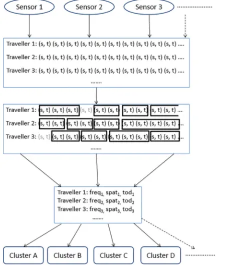
Point-to-point sensor data requires a significant amount of processing before any inferences can be made. As shown inFig. 1, the first step is to collate the data from all sensors according to the unique traveller identifiers. The observations for each traveller then need to be ordered according to the date-time stamps, retaining the sensor number (generically referred to by the variable s) and a

date-time stamp (t).

Next, the time lags between consecutive observations for the same traveller need to be compared in order to determine whether they relate to the same trip. This processing aims to ensure that only devices moving in motorised vehicles are retained in the data. For each pair of sensors, an initial feasibility band is estimated for the time it would take a motorised vehicle to travel directly between the two locations, without making a stop en-route. The midpoint of the feasibility band is a rough estimate of the time it would take to travel on the fastest route between the two sensors, and this was obtained from local off-peak data. Multipliers are then applied to this estimate to obtain upper and lower bounds for the direct travel time. Such multipliers should be specified using local knowledge of the variability in travel times in the area. Any pair of consecutive observations which fall outside of the relevant feasibility band are assumed not to be part of the same trip and therefore are not linked in the data. A second stage is then undertaken which takes into account the travel conditions on the day and at the time when the observations being processed were made. In this stage, observations ofalltravellers at the two relevant detectors around the time of the observations being processed are examined. One example of this type of processing involves the calculation of the following values for each pair of consecutive observations for each traveller:

•

•

These two‘overtaking’values are compared to upper thresholds specified based on local conditions which include the sampling rates of the given data collection tool. For any pairs of consecutive observations which exceed these parameters, the two observations are considered to belong to different trips. The parameters required for processing data in this way are shown inTable 1.

As shown inFig. 1, the output of this process is a set of trip sequences for each traveller, where trips consisting of a single observation have been removed. The trips for each traveller,i, are then analysed to obtain a traveller specific frequency measure (freqi), spatial measure (spati) and time of day measure (todi). A segmentation of the travellers is then obtained using cluster analysis.

The proposed techniques for calculating the repeated trip behaviour measures will now be discussed.

2.1. Trip frequency

All types of point-to-point data collection will result in missing observations. A bias in thetravellerswho can be detected could potentially mean that resulting analyses cannot be considered representative of the population of travellers using the roads of interest. This consideration is outside the scope of the current research. However, missing data may also refer to individual trips which are not detected at all, or an individual sensor not recording all possible data. In the current research, the assumption is made that individual trips are missing at random. This assumption means that for each traveller we have an unbiased, random sample of their trips and so the measure of trip frequency is comparable between travellers. Alternative assumptions could be made if estimates are available of the bias in the trips recorded, for example by type of Bluetooth device or traffic density. In practice, all detectors should be checked to ensure that there were no malfunctions in the study period as this would cause bias which could not easily be adjusted for. In the case study, these checks involved searching within the data for each detector to identify whether there were any substantial time periods when no detections were made. Although this does not cover all possible malfunctions, it was assumed to cover the most common types.

The total number of trips observed per traveller is used as a relative measure of frequency in this paper. While this is assumed to be a comparable measure between travellers, due to missing data it will be an underestimate of travellers’trips passing the sensors. The development of adjustment factors to apply to these measures to get unbiased estimates of trip frequency is left for further research.

2.2. Spatial variability

For spatial variability it is particularly important to focus on the nature of the data. For example,Järv et al. (2014)used mobile phone data and therefore they focused on individuals’activity spaces over time, as opposed to trip data.Bayarma et al. (2007)used data from a six week travel diary and for spatial variability focused on trip duration and the distance of trip destinations from the individuals’homes. Point-to-point sensor data differs from trip data from other sources as it only contains information about the part of the trip within the monitored part of the network, but it can contain many observations, depending on the sensor locations. Therefore, although OD information is not available, entry and exit points to the part of the network which is monitored can be

Table 1

Bluetooth data processing parameters.

captured. Route choices, in terms of the ordered sequence of sensors passed between the entry and exit points, can also be captured. To fully utilise the depth of this spatial information, the methodology in the current paper builds on the work ofDelafontaine et al. (2012), who examined visitor movements through a large trade fair using Bluetooth data. Pairwise Sequence Alignment is used to calculate similarity measures between trips which can then be used to cluster similar trips. The distribution of trips between these spatial clusters for each traveller is then used to assess the degree of spatial variability.

Sequence Alignment was originally developed to compare protein sequences, but has also been used more recently by social scientists and geographers (Abbott, 1995; Shoval and Isaacson, 2007). It is suitable for point-to-point sensor data as it uses all of the available spatial data for a trip and does not just focus on start and end points. It also provides a systematic way of analysing the data while accounting for missing observations within sequences. Sequence Alignment techniques can be separated into global techniques, which try to match entire sequences, and local techniques which seek tofind parts of the sequences which match. Kim and Mahmassani (2015)used one of the latter techniques to identify the Longest Common Subsequences in trace trip data, for example from taxis. Whilst this was a suitable technique in their research as they were aiming to identify‘representative’subsequences for clustering travel patterns, it is not suitable for the current research as it can completely ignore data from the start and ends of sequences.Kim and Mahmassani (2015)also had trajectory data which does not have the same problems with missing observations within sequences as point-to-point data. As inDelafontaine et al. (2012), who also considered point-to-point (Bluetooth) data, global sequence alignment is applied in this paper as it considers the similarities and differences across entire sequences.

In Sequence Alignment, each sequence is represented by a string of letters and then each pair of sequences are aligned. This involves lining up the two sequences one below the other, perhaps with the introduction of gaps, known as indels, in the sequences. A measure of dissimilarity between the two sequences based on a particular alignment is then calculated by comparing each pair of aligned letters.

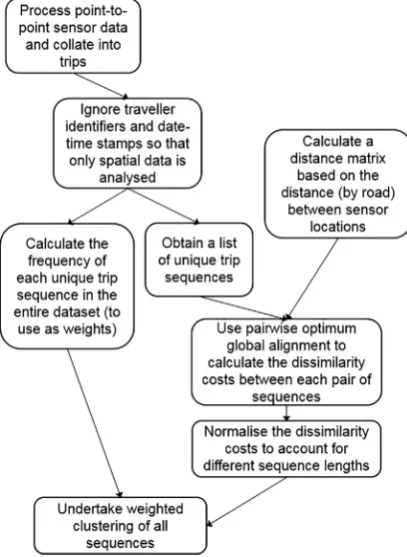
The way in which this research proposes using Sequence Alignment within a methodology for measuring spatial variability of trips is outlined inFig. 2. Firstly the point-to-point sensor data is converted into sequences, where each letter corresponds to an observation at the sensor assigned with that letter. Each sequence corresponds to a trip, i.e. observations which have been matched between sensor locations using a unique identifier, for example a number plate, and then processed to ensure the traveller drove

directlybetween the sensor locations, as described at the start of Section2. The trips for all travellers are then combined and analysed together. The output of this process is a single framework defining different groups of trip sequences across the case study area which is then used to calculate comparable measures for each traveller individually.

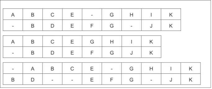
Each pair of trips in the data are compared, through an alignment process, and pairwise costs are calculated based on the similarity between the sequences. For example, consider Sequence 1 (ABCEGHIK) and Sequence 2 (BDEFGJK). There are thousands of possible alignments; three possible alignments are shown inFig. 3.

For each pair of sequences, the optimal alignment is required, namely the alignment with the smallest pairwise cost. Of the

thousands of possible alignments of the sequences inFig. 3, many can be instantly dismissed as suboptimal, such as aligning all of Sequence 1 with indels and all of Sequence 2 with indels. Other alignments can be compared using the pairwise cost which is calculated by aligning sequence x and sequence y and then comparing each pair of aligned letters:

∑

=

Pairwise cost x y( , ) dist x y( , ) i

i i

(1) wheredist x y( , )_{i i} is some sort of distance between the letters in positioniin sequence x and y (xiand yi) with a constant distance used

between an indel and any letter. The distances between each pair of letters are known as substitution costs. The substitution and indel costs are key parameters which determine the optimal alignment of two sequences.

The substitution costs in the current application relate to the dissimilarity between a pair of sensor sites. In Section3, the distance on the shortest path by road between the two sensors is used. The geodesic distance between sensors could have been used, although this would be less useful where there are parallel routes with little opportunity for switching.

A suitable indel cost also needs to be assigned. An indel in a trip sequences could represent a missing observation, either due to a slight difference in route or a genuine missing observation. They are also required when comparing sequences of different lengths. The cost associated with indels should be relatively low so as not to excessively punish missing data, which is common in some types of point-to-point sensor data such as Bluetooth. The indel cost should not, however, be less than half of the distance between the two sensors which are furthest apart, otherwise the optimal alignment process would never align observations from those two sites but would align each observation with an indel instead. In this research, therefore, the smallest indel cost which allows full utilisation of the substitution costs will be used, namely half of the distance between the two sensors in the study which are furthest apart. Indels could represent devices passing a sensor but not being recorded and in this research it is assumed that the probability of this occurring does not depend on whether the device was recorded at the previous sensor. The same indel cost is, therefore, applied to gaps irrespective of whether they are preceded by gaps or letters (denoting observations).

The parameters required to calculate pairwise costs have now been defined, so optimal alignments for each pair of trips can now be identified. Rather than considering all possible alignments in turn, dynamic programming and more specifically the Needleman-Wunsch algorithm (Isaev, 2006, p9) is used tofind optimal alignments and the associated pairwise costs more efficiently. The Needleman-Wunsch algorithm works by creating an array of the costs associated with aligning each letter pair in the two sequences. Therefore, rather than comparing the full sequences in many different ways, the algorithm works efficiently by calculating all possible subsets of the alignments once and then determining the optimal alignment. The algorithm is described in detail, in relation to protein sequence alignment, inNeedleman and Wunsch (1970). An example relating to trip sequences is presented inAppendix A. Where large amounts of data are involved, the optimum alignments should be computed between alluniquesequences to prevent duplicating effort. The optimal alignment for each pair of unique sequences (which represent trips) in the data will have a corre-sponding pairwise cost. A pairwise cost relates to a pair ofsequencesand consists of the sum of the substitution costs for each aligned pair of letters (or a letter-indel alignment). To account for sequences of different lengths, Abbot’s normalisation is applied by dividing each of the optimal pairwise costs by the length of the longer sequence of the pair (Abbott and Tsay, 2000, p13).

∑

=

Normalised pairwise cost x y

dist x y

i ( , )

( , ) i

i i

(2) The optimal pairwise cost represents the spatial similarity between two trips, where partially overlapping routes and geographical closeness are rewarded. These pairwise costs are then used as the distance metric for clusteringallsequences. This is done once, using data from all travellers, so that a consistent measure of‘similar’trips is applied to all, irrespective of how variable the trips for a particular individual are. The clustering is undertaken using weights based on the sequence frequency in the year of data for all travellers as described inStuder (2013). As the number of clusters to use is quite subjective, using hierarchical clustering provides a suitable format of data to identify the most appropriate cut-offto use. After identifying the spatial clusters of trips, each traveller is assessed to see how many of the clusters their trips fall into, and what proportion of their trips fall into their most common spatial

A B C E - G H I K

- B D E F G - J K

A B C E G H I K

- B D E F G J K

- A B C E - G H I K

B D - - E F G - J K

cluster. Despite performing Sequence Alignment and clustering on all trip sequences together, therefore, this process will identify spatial variability measures for each traveller.

In summary, the parameter values and techniques proposed for measuring spatial variability are shown inTable 2.

2.3. Temporal variability

Measures relating to intrapersonal variability in the time of day trips are made need to be comparable across all individuals and should give a meaningful insight into the underlying behaviours. Ideally, temporal variability should be measured based on com-parable trips, but with point-to-point data this is somewhat ambiguous due to the limited coverage of detectors, missing observations and a lack of trip purpose information. For each traveller, trips which arefirst detected at matching sensor locations and are also last detected at matching sensor locations could be compared but these are not guaranteed to relate to the same trip. This is because of the limited spatial coverage of detectors, i.e. these are not the OD pair of the actual trip, and there may be missing data. Also, for each traveller there may be many start and end detector pairs so there would be a confusing array of measures for each traveller, most of which would have very small sample sizes.

An alternative approach, which is used in this paper, is to consider the time of day that an individual passes a particular detector, which for each traveller will be the detector they pass most often. This is somewhat similar to the approach taken byMuthyalagari et al. (2001)on GPS travel diary data. They compare departure times based on the origin or destination of the trip and also based on trip purpose and so obtain measures of variability for thefirst departure from home,final departure from work andfinal arrival at home each day. Using the most common detector location only may be more closely linked to spatial variability as the time they pass a particular point may vary depending on their ultimate destination. It does, however, allow travellers who always travel at the same time of day but go to different locations to be identified in the data.

Having decided upon the observations to compare, a suitable measure of temporal intrapersonal variability needs to be selected. Comparison of observations within time bands can be useful, for example 10 minute intervals were used byMinnen et al. (2015). The results are usually dependent on the (usually arbitrary) choice of time band widths, however, and the relative precision of the time stamps from point-to-point sensors would be wasted. In the current research, therefore, the time of day is treated as a continuous variable and clustering is undertaken for each traveller separately, as was done for public transport users inKieu et al. (2015).Kieu et al. (2015)used a density based clustering algorithm as their aim was to identify the percentage of each traveller’s trips which fall within a habitual time cluster, as opposed to other trips which were classified as noise by the algorithm. This algorithm was not suitable for the current research for two reasons. Firstly, the distribution of the trips classified as noise by a density based algorithm is of interest in this research and therefore a more holistic approach was preferred. Secondly, although the density based clustering algorithm used does not require the specification of the number of clusters to use, it does require minimum points and density reach parameters. These parameters tell the algorithm how close together points should be if they are to be assigned to the same cluster. For example,Kieu et al. (2015)used 5 minutes as their density reach parameter for the time of day of trips analysis. An approach which does not specify such parameters a priori was preferred.

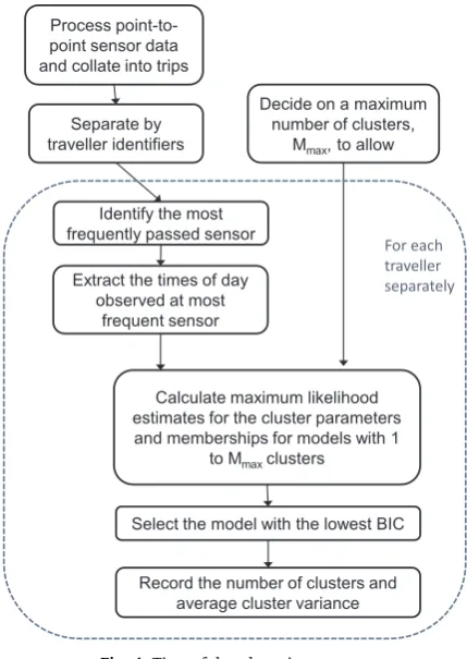
Instead, the current research uses an alternative approach which uses all available data and uses a data driven approach to decide on the spread of clusters, namely Model Based Clustering (seeFraley and Raftery (2002)). This approach assumes that the data is generated according to afinite mixture model, where each component of the probability distribution relates to a cluster. For a given number of clusters, an Expectation-Maximisation algorithm is used to estimate the cluster parameters and memberships with the maximum likelihood (Fraley and Raftery, 2002). The most appropriate number of clusters to use is then determined by comparing a criterion, such as the Bayesian Information Criterion (BIC), between models including different numbers of clusters.

In the current application, the Model Based Clustering is undertaken separately for each traveller, using the process shown in Fig. 4. By representing the times of day an individual passes a given location by a mixture distribution, we are assuming that there are multiple times of day at which an individual passes a given location, for example due to different trip purposes, destinations or preferred arrival times. In Section3, the distribution of the times of day is assumed to be approximately a Gaussian mixture dis-tribution, but more complex formulations are possible (McNicholas, 2016). While a maximum number of clusters must be specified, the number of time of day clusters will vary between travellers. For each traveller, after undertaking the Model Based Clustering, the number of clusters estimated and the variance of those clusters are recorded as the measures of temporal variability.

2.4. Identifying the user classes

Once the measures for the three aspects of repeated trip making have been calculated, namely trip frequency, spatial and temporal Table 2

Proposed parameters to use in the spatial clustering process.

Parameter Proposed value

Substitution cost Distance on the shortest path (by road) between each pair of sensors Indel cost Half of the distance between the two furthest apart sensors Normalisation technique Abbot’s normalisation

Clustering algorithm Hierarchical

variability, each value is standardised prior to the clustering process by subtracting that measure’s mean value and dividing by its standard deviation. In this paper, the followingfive measures of repeated trip making are used, although others could be included:

(i) the number of trips observed in the year,

(ii) the number of temporal clusters estimated based on the time of day the traveller passed their most common sensor location, (iii) the average variance of their temporal clusters,

(iv) the number of spatial clusters their trips were observed in and

(v) the percentage of their trips which fall into their most common spatial cluster.

A number of different clustering methods may be suitable, but in this paper k-means clustering is used. K-means clustering is relatively computationally fast and k-means was also used byBayarma et al. (2007)to identify groups of travel patterns in travel diary data. The choice of clustering method for the case study area is discussed in more detail in Section4.

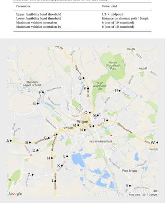
3. Application: a case study in northwest England

In this section the methodology described in Section2is applied to one year of real-life Bluetooth data from the road network in Wigan, a town in Greater Manchester in northwest England. Transport for Greater Manchester (TfGM) has installed around 770fixed Bluetooth detectors next to roads in Greater Manchester. Such detectors are an increasingly popular way to measure travel times on the road network (Aliari and Haghani, 2012; Bhaskar and Chung, 2013; Araghi et al., 2014) and they have also been used to estimate OD matrices (Barceló et al., 2010; Chitturi et al., 2014) and measure pedestrian movements (Bullock et al., 2010; Versichele et al., 2012). Types of Bluetooth-enabled devices include smartphones, laptops, hands-free kits and in-car audio systems. For Bluetooth data, the unique identifiers are known as MAC addresses. By matching these unique identifiers between locations, trip data can be generated andfiltered to remove travel times not associated with motor vehicles. For this case study, the cleaning process was consistent with the approach described in Section2. The parameters used were developed by TfGM and are shown inTable 3.

As only discoverable Bluetooth devices can be detected, the trip data will only be a sample of trips undertaken in the area. The Bluetooth penetration rate has been measured by comparing ANPR and Bluetooth data for one link within Greater Manchester over a twelve hour period and the hourly penetration rates were calculated to be between 16% and 34%.

Data from 23fixed Bluetooth detectors in and around Wigan (Fig. 5) was analysed for all of 2015. The data includes 7,480,204 trips and these trips were associated with 327,264 unique MAC addresses, which for the purposes of this research are assumed to approximately correspond to individual travellers. Almost 28% of these MAC addresses only recorded one trip in this area in the year.

Decide on a maximum number of clusters,

Mmax, to allow Process

point-to-point sensor data and collate into trips

Separate by traveller identifiers

Calculate maximum likelihood estimates for the cluster parameters

and memberships for models with 1 to Mmax clusters

Select the model with the lowest BIC Identify the most

frequently passed sensor

Extract the times of day observed at most

frequent sensor

For each traveller separately

Record the number of clusters and average cluster variance

Just 2% of the MAC addresses recorded greater than or equal to 260 trips in the year, which is equivalent to at least one trip per day, on average, for someone workingfive out of seven days per week.

Computational limitations make Sequence Alignment on all unique sequences observed in the year infeasible, but it is possible for a month of data. To select the most appropriate month to use, the unique trip sequences,seq_k, (wherek=1,…n, the total number of unique sequences) observed in the year of data were extracted. For each of these sequences, the months in which they were observed and the total number of occurrences in the year (wk) were recorded. Eq.(3)was then used to calculate the‘coverage’for each month, l, which is the proportion of all trips in the year which match a trip sequence appearing in monthl. The month of data with the highest coverage should be selected. Only sequences observed in the chosen month will undergo the pairwise alignment process and therefore choosing the month with the highest coverage will maximise the number of trips which can be assigned to a cluster as others will not be represented in the distance matrix.

=∑

∑ = ⎧⎨_⎩

Coverage month l w λ

w where λ

if seq occurs in month l otherwise

1 0 k k kl

k k

kl k

(3) In the case study area, March has the highest coverage (0.98). This means that 98% of the trips in the one year period match trip sequences observed in March. Pairwise Sequence Alignment was undertaken on March data only using the TraMineR package in R (Gabadinho et al., 2011), following the process described in Section2.2and the parameters inTable 4. An indel cost of 3 was used, as

Table 3

Bluetooth data processing parameters used in the case study.

Parameter Value used

Upper feasibility band threshold 1.5 × midpoint

Lower feasibility band threshold Distance on shortest path * 5 mph Maximum vehicles overtaken 6 (out of 10 examined) Maximum vehicles overtaken by 6 (out of 10 examined)

this is half of the distance by road (in miles) between the two sensors which are furthest away from one another, rounded up. After calculating the pairwise costs relating to the sequences, standard hierarchical clustering using Ward’s minimum-variance method was undertaken to create spatial clusters. Ward’s method determines the clusters to merge in agglomerative hierarchical clustering, by minimising the increase in the total within-cluster variance after merging (Ward, 1963).

In order to select the most appropriate number of clusters to use, partition quality measures were calculated, followingStuder (2013). This provided a starting point, but ultimately 150 spatial clusters were used as this provided a useful level of aggregation for the overall intrapersonal variability clustering. The choice of 150 spatial clusters will be discussed further in Section4. A summary of the parameters used in this case study application is provided inTable 4.

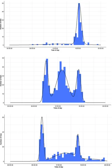
Model Based Clustering was undertaken on the times of day at which each traveller passed their most common sensor location, provided there were at least 20 such observations. After some exploratory analyses, the maximum number of time of day clusters per traveller (Mmax) was set to 9. Temporal clustering could be performed for 33,375 travellers, which is approximately 10% of the travellers observed in the data.Fig. 6includes histograms of the times of day that a sample of three travellers pass their most common sensor. Each plot is overlaid with the estimated Gaussian mixture distribution for the data, which contains two clusters for traveller 1, three for traveller 2 and four for traveller 3. As thefinal intrapersonal variability clustering cannot deal with missing values, travellers with fewer than 20 observations at their most common sensor location were assumed to have one temporal cluster and the average cluster variance was calculated as the variance of the observations, or assigned a zero if there was only one observation.

Five variables were retained for each traveller in thefinal cluster analysis: (i) the number of trips observed in the year,

(ii) the number of temporal clusters estimated based on the time of day the traveller passed their most common sensor location, (iii) the average variance of their temporal clusters,

(iv) the number of spatial clusters their trips were observed in and

(v) the percentage of their trips which fall into their most common spatial cluster.

The percentage of variance explained when using between 1 and 50 clusters were plotted and then the Elbow Method was used to select the most suitable number of clusters of travellers to use. The Elbow Method involves visually identifying the point above which additional clusters bring relatively little gain, in terms of the variance explained, as described inRaschka (2015, Chapter 11) and Sáenz et al. (2011). For this case study that point was at twelve clusters.

3.1. Descriptive statistics for the user classes

Thefinal cluster analysis resulted in twelve clusters of road users which formed three user classes:‘infrequent travellers’ ‘frequent travellers’and‘very frequent travellers’. The clusters will be called subclasses in this paper to avoid confusion with the spatial and the time of day clusters.

Table 5shows that the vast majority of travellers assigned to the‘infrequent’user class recorded very few trips during the year and the average across these six subclasses is just 5 trips in the year. Although the term‘infrequent travellers’has been used, these could be people who were visiting Wigan or local people who do not usually travel by road. The low frequency of observations could also be due to the type of data collection, for example a frequent traveller may only occasionally use their Bluetooth enabled hands-free device and thus appear very infrequently in the data. Very little data is available for these travellers and therefore it is not reasonable to try to make distinctions based on the spatial and time of day variability in trips.Fig. 7demonstrates the uneven distribution of travellers allocated to the clusters, as the infrequent travellers, subclasses A to F, contain 89% of travellers but they only account for 19% of the trips observed.

Within the frequent traveller user class, the four subclasses, G to J, have quite different characteristics as shown inTable 6. They can be separated into two groups based on their trip frequency. Travellers in subclasses I and J are observed almost three times as often as travellers in subclasses G and H. Within each pair, one subclass represents more regular trip makers (H and I) and the other represents less regular travellers (G and J). When the more regular travellers (H and I) are contrasted against their pairwise equivalents (G and J respectively) several features are evident, notably: they make trips to fewer different destinations and/or they have less variation in their route choices (measured in terms of spatial clusters), and they make their most common trip (spatially) a higher percentage of the time. Despite the difference in trip frequency, travellers in both G and J make their most common trip (spatially) approximately 24% of the time. For travellers in H and I this is around 35%, thus they are classed as more regular travellers. Interestingly, the subclasses with higherspatialregularity also have highertime of dayregularity.Table 6shows that the

Table 4

Parameters used in the spatial clustering process in the case study.

Parameter Value used

Substitution cost Distance on the shortest path (by road) between each pair of sensors

Indel cost 3 miles

Normalisation technique Abbot’s normalisation

Clustering algorithm Hierarchical clustering using Ward’s method

subclasses described as being less regular (G and J) have fewer distinct time of day clusters, with greater variances on average. This suggests higher levels offlexibility and lower levels of predictability.Fig. 8highlights the connection between the spatial and time of day variability. In particular it can be seen that travellers in subclasses G and J have a lower percentage of trips in their most common spatial cluster, and also have fewer time of day clusters when compared with their pairwise equivalents (H and I respectively).

Table 5

Road user class and subclass membership and trip characteristics.

User class Subclass Average trips per traveller in 2015 Travellers per subclass Total trips

Infrequent travellers A 1 103,340 153,223

B 3 991 2,767

C 4 86,473 344,128

D 6 4,640 28,127

E 9 23,987 209,480

F 10 72,042 720,326

Frequent travellers G 69 16,634 1,144,115

H 100 8,163 820,221

I 264 3,089 815,504

J 274 5,809 1,590,437

Very frequent travellers K 685 1,901 1,302,874

L 1,790 195 349,002

A to F

A to F

K L

0%

20%

40%

60%

80%

100%

Travellers

Trips

Fig. 7.Segmentation of trips and travellers into subclasses.

Table 6

Characteristics of frequent traveller subclasses.

Spatial variability Time of day variability

Subclass Average trip freq. Overall Average number of spatial clusters used

% of trips in most common spatial cluster

Overall Average number of time of day clusters

Average variance

G 1-2 per week Less regular 21 24% Less regular 1.4 0.015

H 1-2 per week More regular 17 36% More regular 3.5 0.004

I 5 per week More regular 26 34% More regular 6.4 0.003

J 5 per week Less regular 41 24% Less regular 2.6 0.009

trips observed. Subclasses K and L contain travellers who record 2 and 5 trips per day on average respectively. Subclass L has far fewer travellers allocated to it than any other cluster (just 195). The very frequent travellers havetime of day variabilitycharacteristics which are similar to the average of subclasses I and J, which are the travellers with higher trip frequencies within the‘frequent’user class. The very frequent travellers make a wider variety of trips (spatially), than travellers in I and J, but the amount of spatial variability does not increase at the same rate as the trip frequency. Subclasses I and J have 7.6 trips per spatial cluster on average, but subclasses K and L have 11.7 and 18.7 respectively. Therefore, as well as making more trips than other travellers, these very frequent travellers also have different spatial characteristics.

3.2. Predictable differences in user class proportions

Identifying predictable differences in the proportion of trips in each road user class by the day of the week or season could help to identify systematic differences in travel behaviour, which could inform policies which differ systematically as discussed inCrawford et al. (2017). The proportions are relatively stable across days of the week and seasons in this case study area, although some patterns are evident. For example, infrequent travellers are slightly more common on weekend days (seeFig. 9) which is consistent with Wigan being a trip attractor for weekend activities such as visiting a park, museum or theatre. The proportion of trips made by very frequent travellers is also higher on weekend days than on weekdays. This is particularly surprising on Sundays when there are likely to be fewer buses operating and fewer deliveries being made. For all three user classes, the difference in proportion between weekdays and weekend days is statistically significant (p < 0.00001).

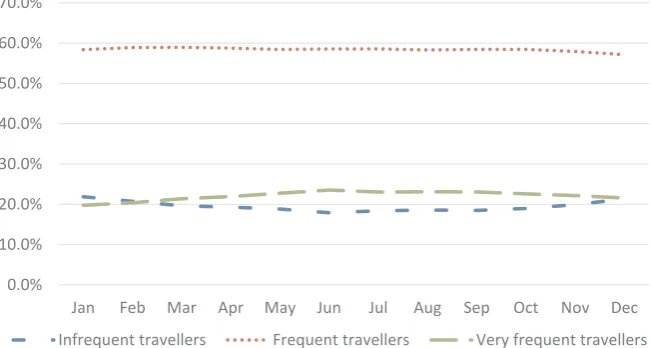
Frequent travellers contribute a consistent proportion of trips throughout the year. The proportion is highest at 59.0% in March but remains relatively stable until there is a decrease to 57.1% in December, probably due to the holiday period. As shown inFig. 10,

20.1%

20.4%

19.3%

56.7%

56.4%

58.9%

23.2%

23.1%

21.8%

0%

20%

40%

60 %

80%

100 %

Sat

Sun

weekday average

Infrequent

Frequent

Very frequent

Fig. 9.Proportion of trips by each road user class in Wigan by the day of the week.

0.0%

10.0%

20.0%

30.0%

40.0%

50.0%

60.0%

70.0%

Jan

Feb

Mar

Apr

May

Jun

Jul

Aug

Sep

Oct

Nov

Dec

Infrequent travellers

Frequent travellers

Very frequent travellers

the proportions of trips made by infrequent and very frequent travellers vary more throughout the year. For both infrequent and very frequent travellers, the differences in the proportion of trips made by the user class in January and June are statistically significant (p < 0.00001). For frequent travellers, the same comparison is also statistically significant at the 0.05 significance level (p = 0.048), although less convincingly so. A higher proportion of trips are made by infrequent travellers during the winter months. This could be because the leisure trip attractors in the town are more likely to relate to indoor activities, whereas during the summer there may be more competition from outdoor activities which are not within the monitored area of Wigan. It could also be due to an increased reliance on cars during months when the weather is colder and wetter. The proportion of trips made by very frequent travellers peaks during the summer months. This, together with the day of the week analysis, suggests that the very frequent traveller user class is more closely linked to leisure trips than business trips. The current case study is limited as only one year of data was analysed and therefore it is not clear whether the increase in the proportion of trips made by very frequent travellers between January and June is part of a longer term trend, for example an increasing number of taxis operating in the area, or whether it is truly a seasonal pattern.

4. Discussion

Although the trip frequency measure was designed to be a comparative value, it is inevitable that attempts will be made to interpret the user class characteristics using this measure. Asfixed Bluetooth detectors do not have a 100% detection rate for discoverable Bluetooth devices and trips could be missed due to not carrying the device or disabling the Bluetooth functionality, the trip frequency data should be considered to be a lower bound for the number of trips actually made. There may also be a bias due to new technologies, for example iPhones from iOS 8 have features which can randomise MAC addresses (the“unique”identifiers) to prevent the tracking of devices. As the data analysed in Section3is from 2015, the penetration rate of such devices is assumed to be small. In the future, analyses relating to repeated trip making using Bluetooth data may require additional data collection to un-derstand the types of devices being detected and the possible implication for trip frequency measures.

The trip frequency values will be sensitive to the parameters used in cleaning the Bluetooth data, particularly those used as part of the process to link together observations into trips. In the application to one year of data in Section3, for example, 0.4% of the trips observed were circular routes which included at least three observations. Whilst it is virtually impossible to distinguish a very brief drop-offon a route from a stop at a pedestrian crossing, for example, further work should focus on identifying the optimal parameter values for connecting or splitting trip data.

Some of the circular routes may also be a subset of the trips recorded by taxis or private hire vehicles which are either waiting for customers or serving customers then returning to a base such as a train station. As the purpose of this methodology is to classify all motorised road users, it is important that such vehicles are included in the analysis; indeed, it may be of interest to identify users who are often circling within parts of a city. These travellers could be identified by adding additional measures into the overall clustering process. These could include the proportion of trips which pass the same detector more than once, or the average‘trip’length. Adjustments may then be required to the user class proportions in order to account for the higher sampling rate for these users, if local research has identified that taxis and private hire vehicles are more likely to be detected by Bluetooth detectors than other vehicles.

The Sequence Alignment based method was used to identify 150 spatial clusters from the trips observed. Each cluster contains 173 different sequences on average. The heterogeneity of spatial cluster membership is highlighted by the variety in the number of unique sequences assigned to each spatial cluster and the variability in sequence lengths and starting sensor location within clusters.Fig. 11 shows the 15 most common sequences, out of 197, in one spatial cluster. These sequences are each observed between 127 and 893 times in the year of data. The sequences go from the west of Wigan to the east via the town centre. The sequences relate to one spatial cluster only and demonstrate the effectiveness of the method in combining trip sequences where intermediate sites are not observed and those representing slightly different routes, for example trips going past site S or site R.

The choice of 150 spatial clusters was made by initially considering measures of the‘quality’of each partitioning of the data as described inStuder (2013), but also using a more qualitative examination of the trip sequences clustered together. Plots of a range of partition quality measures, including the Average Silhouette Width1(which compares distances from an observation to observations in the same cluster and in other clusters) and the Calinski-Harabasz index (which is based on the F statistic used in ANOVA), showed apparent step changes at around 150, 800 and 2000 clusters. An examination was undertaken of 3 clusters randomly selected at the 150 cluster level to explore whether the clusters at the 800 cluster level were more intuitive. In one case, 95% of the sequences were assigned to a single cluster at the 800 cluster level. In another case, 94% of the trip sequences were split between two clusters at the 800 level, but the separation was not particularly meaningful. The most common sequences in the two clusters were from site W to site R and from site W to site N, which are similar trips but with different sequence lengths. In the third case, the three largest clusters at the 800 cluster level did have meaningful differences: one included trips travelling north to P, one included the reverse trips (travelling south from P) and the other included trips with at least two sites in common with the north-south trips, but which ultimately travelled east-west or further north. This examination was very subjective but it highlights the difficulty in selecting the

‘right’level of aggregation overall. In practice, however, a choice has to be made which gives the most meaningful results overall. The final user class clustering was repeated using the spatial variability measures calculated using 150, 800 and 2000 spatial clusters and the characteristics of the twelve clusters were relatively similar. For example, if we compare using 150 and 2000 spatial clusters: the percentage of trips by frequent travellers remained fairly constant, the percentage of trips byinfrequent travellers increased from

19.5% to 20.6% and the percentage of trips by very frequent travellers decreased from 22.1% to 21.0%. This suggests that the overall methodology is fairly robust with respect to the number of spatial clusters selected.

As discussed in Section2.2, an indel cost of half of the distance between the two furthest apart sensors provides a balance between penalising sequences with missing data and utilising the full range of substitution costs, which in the current application are the shortest distances by road between pairs of sensors. The spatial clusters obtained are sensitive to this parameter choice. Increasing the indel cost further in the case study area would have reduced the likelihood of clustering together sequences of different lengths. For example, only 7% of clusters contained sequences which were all the same length when an indel cost of 3 was used, but this increased to 68% if the indel cost was increased to 5.8 (the largest distance between two sensors). Therefore, to utilise all of the data in the substitution cost matrix and also to prevent clusters being formed on the basis of trip sequence length, an indel cost of 3 appears to be reasonable for the case study. The sensitivity of the spatial clusters to the indel cost should be utilised by the modellers in future applications to tune the algorithm to their data.

Approximately 10% of the travellers observed in the data had sufficient data to be able to produce a measure of intrapersonal variability for the time of day they pass their most common location. This percentage is determined by the minimum sample size specified for the Model Based Clustering. This parameter has been set quite low in this case study, at 20, and therefore reducing it further was not feasible. For the travellers with sufficient trips passing their most common sensor location, the proportion of their total trips that this measure represents varies; 29% of these travellers passed their most common location on less than 50% of their trips. This means that for some travellers, their most common detector sites are more important in terms of describing their overall travel patterns in Wigan than for other travellers. This will ultimately mean that the measure of temporal variability will be more representative of time of day variability in travel for some people than for others, although it is the most reasonable estimate to make, given the data available. Also, although visual inspections were undertaken for a sample of travellers, further work is required to determine whether the Gaussian assumption is reasonable, or whether another distribution, perhaps a skewed distribution such as the lognormal distribution, would be more appropriate.

The choice of k-means as the clustering algorithm may have an impact on thefinal clusters, and thus user classes, identified. Due to the large number of travellers in Section3, standard hierarchical clustering is not possible due to computational limitations. An alternative algorithm which was also applied to the case study is the density-based algorithm DBSCAN (Ester et al., 1996). DBSCAN can identify clusters of arbitrary shape using very few initial parameters. DBSCAN was applied to the year of data analysed in Section 3, but the results were less satisfactory than those obtained using k-means. DBSCAN identified one very large cluster, which ap-proximately equated to the infrequent traveller user class using k-means. Irrespective of the parameters applied, this technique resulted in many very small clusters which is not useful when defining user classes. Also, although it is considered an advantage that DBSCAN can identify noise in the data, it is somewhat problematic in the current application as 4% of travellers were not assigned to

A

-B-

M

-

N

-

R

-

T

-

W

A

-B-

G

-

M

-

N

-

R

-

T

-

W

A

-B-

N

-

R

-

T

-

W

B-

G

-

M

-

N

-

R

-

T

-

W

A

-B-

M

-

N

-

R

-

W

A

-B-

G

-

N

-

R

-

T

-

W

A

-B-

R

-

T

-

W

A

-B-

M

-

R

-

T

-

W

A

-B-

R

-

W

A

-B-

N

-

R

-

W

A

-B-

M

-

R

-

W

A

-B-

M

-

N

- -

S

W

A

-B-

M

-

N

- -

S

T

-

W

A

-B-

G

-

M

-

R

-

T

-

W

A

-B-

G

-

M

-

N

-

R

-

W

a cluster. It was therefore preferable to use k-means clustering for this particular case study, but alternative algorithms should still be explored in future applications.

The overlap between some of the k-means clusters and the slightly different clusters identified by DBSCAN suggest that it may be more appropriate to use fuzzy, rather than hard, clustering to identify traveller user classes and subclasses. For example,Chiang et al. (2003)have used fuzzy clustering to account for the fact that some air travel passengers have characteristics relating to more than one market segment. Non-fuzzy clustering has been used in the current paper as it provides results which are more intuitive for policy analyses as travellers belong to a single user class, but fuzzy user classes could be used in future applications.

5. Conclusions

This study has demonstrated the extent to which road user classes based on repeated trip making behaviour can be identified using point-to-point sensor data. The methodology was designed for a specific type of data, namely point-to-point sensor data, and non-traditional techniques, from a transportation research perspective, have been used to extract as much relevant data as possible. The Bluetooth data analysed for the case study area was collected for the purpose of travel time estimation and therefore the marginal costs of using it for this research were minimal.

The results obtained from the proposed method could be used by policy makers and practitioners in several ways. The most direct uses are to gain a better understanding of road users in an area and to inform other forms of data collection. For example, the user classes could be used as a framework within which to recruit survey participants to ensure that the full range of road users are included. It may also raise questions which could be included in user focus groups or surveys. It may also highlight where more in-depth examination is required. For example, now that an infrequent traveller user class has been defined, road managers may wish to explore whether this user class makes up a greater proportion of travellers on specific days where there are seasonal sales, sporting events or major incidents on other roads in the region. Such insights could inform planning for future special events. User classes may also inform more general policy development and could be used as inputs for economic or behavioural models.

In the case study, the majority of trips are made by frequent travellers (58%) but the vast majority are not detected making two trips per weekday, on average, as we might have expected if we assumed that most travellers follow a regularfive out of seven workdays working pattern, although further research is required to determine the proportion of a traveller’s trips which are detected by Bluetooth sensors. With this information, transport planners can determine the extent to which these‘frequent’travellers would be likely to benefit from discounts due to weekly or monthly public transport tickets. The subclasses with different levels of spatial and temporal variability would then be relevant in determining alternative transport options. For the frequent travellers with lower intrapersonal variability ride sharing may be a suitable option to promote, although the ability to make a significant proportion of trips to other locations should also be addressed. For the frequent travellers with greater intrapersonal variability alternative options with moreflexibility might be more attractive, for example cycling or car clubs.

For the travellers in the very frequent user class, further research is required to examine what sort of trips are being recorded, as the higher proportion of trips at the weekend and during the summer suggest that it is not just related to taxis, buses and delivery drivers. If they are predominantly business trips, then policies promoting mode change for personal travel will not result in a decrease in the 22% of trips made by these very frequent travellers. To have any impact on the trips made by this user class, alternative policies would need to be considered, for example changes to bus routes or encouraging consolidated deliveries.

Acknowledgements

The research is funded by the UK Engineering and Physical Sciences Research Council and Highways England through an Industrial CASE Ph.D. Scholarship (grant number EP/K504440/1). The author would like to thank Transport for Greater Manchester for allowing access to the data used in this research. An earlier version of this paper was presented at the Universities’Transport Study Group conference in Dublin (2017) and the authors are grateful for feedback provided by attendees. The authors would also like to thank the anonymous referees for their comments.

Appendix A

The Needleman-Wunsch algorithm can be used to find optimal alignments between two sequences relatively efficiently by aligning all possible subsets of the sequencesfirst. This appendix willfirstly include an overview of the process involved infinding the optimal alignment of generic Sequences 1 and 2. An example of the process will then be provided using the two example sequences from Section2.2.

The algorithm has three stages. Firstly, a table is created which will be used to record the costs associated with all of the partial alignments undertaken. The table should have Sequence 1, preceded by an indel, as the column headings and Sequence 2, preceded by an indel, as the row headings. The top left cell should be populated with a zero.

show whether the smallest cumulative cost was generated using the value from the cell above, to the left, or diagonally to the left. In the third stage, the completed table is examined in order to extract the total pairwise cost associated with the optimal alignment of the two complete sequences, and the optimal alignments themselves. The optimal cost of aligning Sequence 1 and Sequence 2 is simply the value in the bottom right hand cell of the table. The optimal alignment can be found by tracing back the arrows connecting thisfinal cell with the top left hand cell (in which a zero was entered).

A.1. Example 1

The algorithm is best illustrated by an example. Consider Sequence 1 (ABCEGHIK) and Sequence 2 (BDEFGJK) from Section2.2. For this example let us assume that the substitution costs (i.e. the‘distance’between a pair of letters) are determined by their order in the alphabet. For example, comparing A with A gives a cost of 0, and comparing A with Z gives a cost of 25. This is related to the current application as the letters A to K could represent evenly spaced Bluetooth detectors in alphabetical order along a corridor containing many entrances and exits.

As well as the substitution costs, the indel cost also needs to be specified. In thefirst example, the indel cost is set at half of the distance between the furthest apart letters, which are A and K in this example. The indel cost is, therefore, set at 5.

In stage 1, the table shown inFig. 12is created.

In stage 2, the table is populated. An example of a cell which requires populating is shown inFig. 13. The three options for populating the cell marked with an X are:

a. Aligning letters A and B. This would involve taking the top left diagonal cell (0) and adding on the substitution cost between A and B, which are one letter apart, giving a total of 1.

b. Adding an indel to Sequence 1 to align with letter B in Sequence 2. This would involve taking the cell above (5) and adding on the indel cost (5) to give a total of 10.

c. Adding an indel to Sequence 2 to align with letter A in Sequence 1. This would involve taking the cell to the left (5) and adding on the indel cost (5) to give a total of 10.

The smallest possible value is, therefore, 1, which is entered into this cell, with an arrow pointing to it from the top left diagonal cell, to show which the optimal alignment option was. The same process is repeated for each cell, working along each row from left to right, starting with the top row and moving down.Fig. 14shows the completed table.

In stage 3, the optimal pairwise alignments and the associated cost are identified. In this example, the pairwise cost associated with the optimal alignment is 9 (the value in the bottom right hand cell). Tracing back the arrows from this cell to the top left hand cell shows the optimal alignment, as shown inFig. 15.

Table 7

Alignment options for each letter pair.

Option Previous value taken

froma

Value added

Aligning the two letters Top left diagonal Appropriate substitution cost for the letters in the column and row headings for this cell

Adding an indel into the sequence in the column headings (Sequence 1)

Cell above Indel cost

Adding an indel into the sequence in the row headings (Sequence 2)

Cell to the left Indel cost

a _{If there is no value in the given cell, for example cells in the top row do not have a cell above them, then the relevant option is unavailable.}

Using the substitution and indel costs described above, the optimal alignment corresponds to the second alignment suggested in Fig. 3namely:

A B C E G H I K

- B D E F G J K

After calculating optimal alignment costs, but prior to undertaking the spatial clustering, the alignment costs need to be normalised so that long sequences are not disproportionately punished for mismatches. In Section2.2, Abbott’s normalisation is proposed, which involves dividing the pairwise cost by the length of the longest sequence in the pair. In this example, dividing 9 (the optimal pairwise cost) by 8 (the length of Sequence 1) gives the normalised pairwise cost of 1.125.

A.2. Example 2

The optimal alignment obtained will depend upon the substitution and indel costs used. Using the same sequences as in Example 1,Fig. 16demonstrates the output of the algorithm if an indel cost of 1 was used, instead of 5.

In this example, the total pairwise cost is 5 and the normalised pairwise cost is 0.65. The branching out of the red arrows indicates that there are multiple possible alignments with this optimal cost. The two possible alignments are both included inFig. 3:

Fig. 13.Example of cell completion.

Fig. 14.Stage 2 of the Needleman-Wunsch algorithm.

A B C E G H I K

- B D E F G J K

A B C E - G H I K

- B D E F G - J K

Multiple optimal alignments are not problematic in the current application as only the total pairwisecostof the optimal alignment is required for the clustering process.

References

Abbott, A., 1995. Sequence analysis: new methods for old ideas. Ann. Rev. Sociol. 21, 93–113.

Abbott, A., Tsay, A., 2000. Sequence analysis and optimal matching methods in sociology: review and prospect. Sociol. Methods Res. 29, 3–33.

Aliari, Y., Haghani, A., 2012. Bluetooth sensor data and ground truth testing of reported travel times. Transp. Res. Rec.: J. Transp. Res. Board 2308, 167–172.

Antoniou, C., Balakrishna, R., Koutsopoulos, H.N., 2011. A Synthesis of emerging data collection technologies and their impact on traffic management applications. Eur. Transp. Res. Rev. 3, 139–148.

Araghi, B.N., Olesen, J.H., Krishnan, R., Christensen, L.T., Lahrmann, H., 2014. Reliability of bluetooth technology for travel time estimation. J. Intell. Transp. Syst. 19, 240–255.

Axhausen, K.W., Zimmermann, A., Schönfelder, S., Rindsfüser, G., Haupt, T., 2002. Observing the rhythms of daily life: a six-week travel diary. Transportation 29, 95–124.

Barceló, J., Montero, L., Marqués, L., Carmona, C., 2010. Travel time forecasting and dynamic origin-destination estimation for freeways based on bluetooth traffic monitoring. Transp. Res. Rec.: J. Transp. Res. Board 2175, 19–27.

Bayarma, A., Kitamura, R., Susilo, Y., 2007. Recurrence of daily travel patterns: stochastic process approach to multiday travel behavior. Transp. Res. Rec.: J. Transp. Res. Board 2021, 55–63.

Bhaskar, A., Chung, E., 2013. Fundamental understanding on the use of Bluetooth scanner as a complementary transport data. Transp. Res. Part C: Emerg. Technol. 37, 42–72.

Buliung, R.N., Roorda, M.J., Remmel, T.K., 2008. Exploring spatial variety in patterns of activity-travel behaviour: initial results from the Toronto Travel-Activity Panel Survey (TTAPS). Transportation 35, 697–722.

Bullock, D., Haseman, R., Wasson, J., Spitler, R., 2010. Automated measurement of wait times at airport security. Transp. Res. Rec.: J. Transp. Res. Board 2177, 60–68.

Chen, R., Mahmassani, H.S., 2004. Travel time perception and learning mechanisms in traffic networks. Transp. Res. Rec.: J. Transp. Res. Board 1894, 209–221.

Cherchi, E., Cirillo, C., 2