Quantum computation with realistic magic-state factories
Joe O’Gorman1and Earl T. Campbell2
1Department of Materials, University of Oxford, Oxford OX1 3PH, United Kingdom 2Department of Physics and Astronomy, University of Sheffield, Sheffield S3 7RH, United Kingdom
(Received 26 August 2016; published 31 March 2017)
Leading approaches to fault-tolerant quantum computation dedicate a significant portion of the hardware to computational factories that churn out high-fidelity ancillas called magic states. Consequently, efficient and realistic factory design is of paramount importance. Here we present the most detailed resource assessment to date of magic-state factories within a surface code quantum computer, along the way introducing a number of techniques. We show that the block codes of Bravyi and Haah [Phys. Rev. A 86,052329 (2012)] have been systematically undervalued; we track correlated errors both numerically and analytically, providing fidelity estimates without appeal to the union bound. We also introduce a subsystem code realization of these protocols with constant time and low ancilla cost. Additionally, we confirm that magic-state factories have space-time costs that scale as a constant factor of surface code costs. We find that the magic-state factory required for postclassical factoring can be as small as 6.3 million data qubits, ignoring ancilla qubits, assuming 10−4error gates and the
availability of long-range interactions. DOI:10.1103/PhysRevA.95.032338
I. INTRODUCTION
Architectures for quantum computers must tolerate ex-perimental faults and imperfections, doing so in the most practical and efficient way. One aspect of fault tolerance is the use of error-correcting codes, which provides a storage method for protecting quantum information from noise. To perform quantum computations, additional techniques are needed to ensure a universal set of quantum gates can be implemented fault tolerantly. Most error-correcting codes natively allow fault-tolerant implementation of gates from the Clifford group, a nonuniversal set of gates. Fully functional quantum computation is attained by adding the Toffoli orπ/8 phase gate to the Clifford group. The prevailing proposal for performing these gates is to first prepare high-fidelity magic states, which are then used to inject a gate into the main computation. These magic states are needed in vast quantities, and their preparation requires a significant portion of a device to operate as a dedicated magic-state factory [1–3]. Alternatives exist to the magic-state paradigm [4–10], but it is unclear whether they will be feasible substitutes due to worse thresholds [11,12].
Magic-state factories use several rounds of distillation protocols, and several directions have been explored [15–20] to improve efficiency over the original proposal which uses Reed-Muller codes [1]. Notably, an n→k block protocol takesninput magic states and outputkat higher fidelity, with higher ratios ofn to k generally offering greater efficiency [15–17]. These block protocols do require more complex circuits, but there has been limited investigation into the full resource cost of these protocols. One advance in this direction [3] has shown that block protocols can be realized
Published by the American Physical Society under the terms of the Creative Commons Attribution 4.0 International license. Further distribution of this work must maintain attribution to the author(s) and the published article’s title, journal citation, and DOI.
in constant time, independent ofk, by braiding defects in the surface code. Despite this, the same work found that efficiency improvements of block protocols were modest. However, all previous work has taken a very pessimistic estimate of the fidelity of these protocols, leading to an overestimated cost. We present several results improving resource costs and leading to a more optimistic outlook for realzing magic-state factories.
We present a method of realizing the Bravyi-Haah block protocols [16] in constant time without relying on braiding operations, providing a fast implementation to other architec-tures. Braiding operations natively support control-NOT(CNOT) gates with multiple target qubits in constant time, which is the key step in the circuit reduction of Ref. [3]. Our approach does not require availability of such powerful gates, but rather reduces time costs by borrowing concepts from subsystem codes [21–24] and notions of gauge fixing [7,9,25]. In subsystem codes, operations acting on many qubits are broken up into more pieces each involving fewer qubits, which we find enables greater parallelization in realizing Bravyi-Haah. Our proposal is especially applicable to distributed architectures for quantum computation and provides these devices with an approach to magic-state distillation that is low in ancilla and time costs.
We also show that magic-state factories can make more use of block protocols than previously thought by using techniques to reduce and calculate the global output error. Consider a protocol outputting K qubits with multiqubit global error rate g. All previous studies have used the union bound, also called Boole’s inequality, to assert g K, where K is the number of magic states and is the average error rate of single-qubit outputs, obtained by tracing the qubit from the multiqubit state. For an uncorrelated product state,
ρg =ρ⊗K, we have g =1−(1−)K, so to leading order
g =K−O(2), and the union bound is a good estimate for small. However, the output of block protocols can be highly correlated. Boole’s inequality holds for correlated states, but
clusters of errors can go undetected and lead to a correlated error pair. If one error is present, it almost certainly has a partner. As such, use of the union bound has led to systematic overestimation of noise in Bravyi-Haah and other distillation protocols. Here we track these correlations through multiple rounds of a magic-state factory. We take as our starting point the triorthogonal codes for producingπ/8 magic states [16] and a method of producing Toffoli magic states [26,27]. Once we begin tracking correlations, it becomes apparent that quality control of the factory can be improved. Detecting an error in one part of the factory can, due to correlations, indicate a likely undetected partner error elsewhere in the factory. We introduce the notion of module checking whereby we discard magic states brought into disrepute by their correlated partners. The enhanced fidelity of module checking is both analytically estimated and found by numerical Monte Carlo simulations, with excellent agreement between these methods.
The specification of the distillation protocol is just one as-pect of designing magic-state factories. The size of magic-state factories depends on both the distillation protocols and also the underlying error correction codes, and a significant saving can be made by judiciously reducing the error correction code at earlier rounds of magic-state distillation. The balanced investment of qubits at each round of distillation uses small surface codes for low-fidelity magic states and larger surface codes for high-fidelity magic states. A small fraction of magic states in the factory will be high fidelity and require much larger surface codes. Raussendorf et al. [28] argued that, consequently, magic-state distillation can be achieved at a constant factor cost over surface code error correction, which we also observe and discuss.
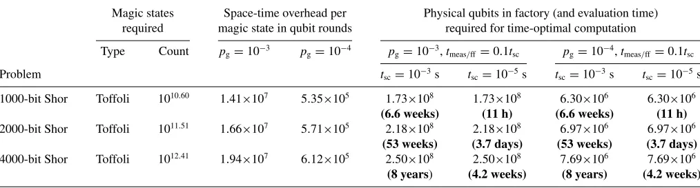
Taking all factors into consideration, we present a blueprint for a factory capable of delivering enough magic states to solve large Shor’s algorithm tasks, beyond the reach of classical computation, within a surface code quantum computer. Our results are summarized in TableI, where we look at both the space-time overhead required to produce a Toffoli magic state and the physical footprint of the factory required to produce
magic states at an average rate that can just keep up with the “time-optimal” surface code implementation of the algorithm [14], which we further discuss in Sec.VI.
II. REALIZING BLOCK PROTOCOLS
Many descriptions of distillation protocols are high level, leaving open many aspects of how to implement these proto-cols. To assess the full resource cost, we require a low-level description of distillation protocols in terms of elementary operations, such as one- and two-qubit gates, preparations, and measurements. We call such a description a realization of a protocol, and a given protocol can have different realizations with varying costs.
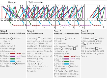
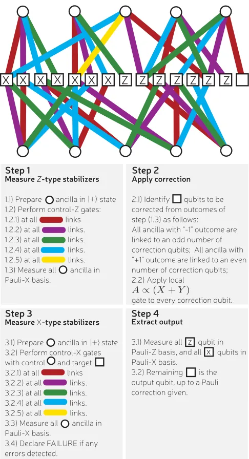
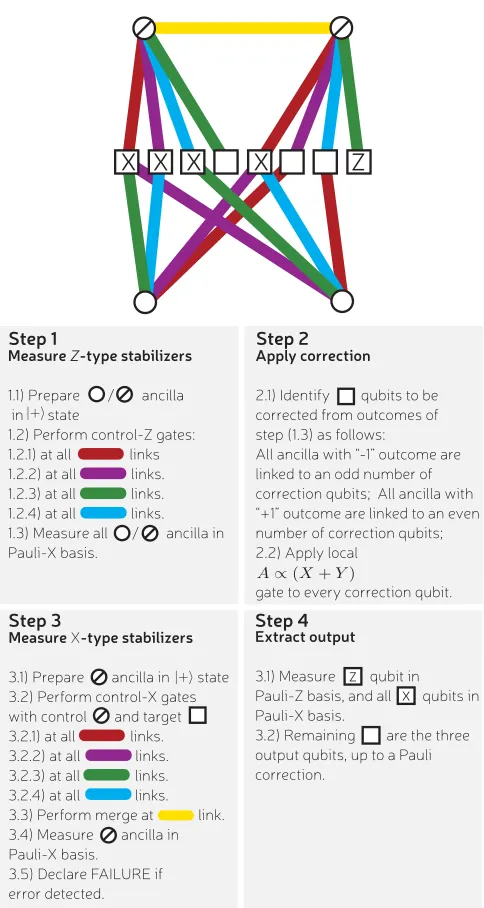
This section presents a realization of the Bravyi-Haah protocols, giving explicit instructions presented in Fig.1. The protocol is presented as a four-step process acting on a col-lection ofnnoisy|Tstates, where|T ∝ |0 +exp(iπ/4)|1. The first step uses ancillas to measure operators composed of Pauli-Z operators, and the second step applies a correction dependent on the measurement outcomes. The third step uses ancillas to measure operators composed of Pauli-X
[image:2.608.50.557.615.752.2]operators, with only certain measurement outcomes kept. After a successful third step, thekoutput magic states are within an encoded state and delocalized across 3k+8 sites. The fourth step uses measurements to localize the output qubits to specific sites. All these steps are detailed in Fig. 1 and show how the multiqubit measurements are broken down into ancilla preparation, two-qubit gates, and single-qubit measurements. Observe in Fig.1that each multiqubit measurement involves only four entangling gates, with each such gate designated a distinct colored link. Therefore, the measurement is a four-qubit operator. This is called the weight of the operator. When using a single ancilla to measure a stabilizer of weightm, we needmtime steps to perform the required controlled-gate operations. The low, and constant, weight of our measurements gives the realization a constant time cost. More commonly, the Bravyi-Haah protocol is presented as requiring only two
TABLE I. The size and time requirements of some examples of magic-state factories. We consider an implementation of Shor’s algorithm requiring 40N3Toffoli gates, which dominates the overhead. We realize each of these gates using a single Toffoli magic state or sevenT states
in parallel [13], whichever proves optimal. In this algorithm, the Toffoli gates are all sequential, so using time-optimal methods [14], the fastest possible run time is 40N3t
meas/ff, wheretmeas/ff is the time taken to make a physical measurement and feed forward the result to selectively
perform a single-qubit gate elsewhere in the quantum computer. The number of “physical qubits in factory” neglects qubit cost associated with measuring surface code stabilizers, so for many architectures this number will be doubled. The variabletscis the time taken to perform
a single round of the parallel stabilizer measurements of the surface code, a process involving fourCNOTgates, two single-qubit gates and a measurement. We assume throughout thattmeas/ff=0.1tsc, which is reasonable for a distributed architecture such as ion traps.
Magic states Space-time overhead per Physical qubits in factory (and evaluation time) required magic state in qubit rounds required for time-optimal computation
Type Count pg=10−3 pg=10−4 pg=10−3,tmeas/ff=0.1tsc pg=10−4,tmeas/ff=0.1tsc
Problem tsc=10−3s tsc=10−5s tsc=10−3s tsc=10−5s
1000-bit Shor Toffoli 1010.60 1.41×10⁷ 5.35×10⁵ 1.73×10⁸ 1.73×10⁸ 6.30×10⁶ 6.30×10⁶
(6.6 weeks) (11 h) (6.6 weeks) (11 h)
2000-bit Shor Toffoli 1011.51 1.66×10⁷ 5.71×10⁵ 2.18×10⁸ 2.18×10⁸ 6.97×10⁶ 6.97×10⁶
(53 weeks) (3.7 days) (53 weeks) (3.7 days) 4000-bit Shor Toffoli 1012.41 1.94×10⁷ 6.12×10⁵ 2.50×10⁸ 2.50×10⁸ 7.69×10⁶ 7.69×10⁶
FIG. 1. Explicit circuit for realizing Bravyi-Haah (3k+8)→kblock protocols fork=2,6,10,14, . . . .Squares indicate the (3k+8) noisy
|Tmagic states to be distilled, and circles represent ancilla qubits used to effect measurements on the magic states. Increasingkdoes not increase the number of time steps in the protocol but increases the number of qubits involved in a block. As we increasek, we add qubits to the tail end, with the protocol translationally invariant along the tail. We report that we have independently confirmed the validity of the protocol fork=2 by full wave-function simulation, which further confirmed that all single errors are detected and all two errors processes lead to outputs with correlated errors.
measurements ofX-type observables that have weight 2k+4, implying a potentially expensive time cost. However, the concept of gauge subsystem codes provides a method whereby such complex measurements can be broken down into a larger number of simpler measurements [21–24]. In AppendixCwe present a rigorous demonstration that the Bravyi-Haah code can be viewed as a subsystem code, and using a combination of gauge fixing and a cat-state ancilla, we create a circuit of depth 4 for both X and Z measurement sets. We call this general approach gauge-MSD, where MSD is short for magic distillation. We remark that constant time realization was also found by Fowleret al.[3] but was tied to a monolithic braiding architecture.
The time complexity of our realization is simply
tblock =8tcnot+tA+2tprep+3tmeasure∼8dtsc, (1)
where tcnot is the two-qubit gate (e.g., CNOT) time, tA is
the gate time for single-qubit A=(X+Y)/√2 rotation,
tprep is the single-qubit preparation time, and tmeasure is the
single-qubit measurement time. Here all operations are applied fault tolerantly to logical qubits within an error-correcting code. Therefore, the time scales are for fault-tolerant gates. We will assume throughout that logicalCNOTgates are applied transversally and thus take timetcnot=tg+d×tsc, wheretg
is the time for the physical gate,dis the code distance, andtsc
is the time for a round of stabilizer measurements. Therefore, for large distances the time is dominated by 8dtsc. We will
also take this as the time cost of a merge operation [29,30] which we use to project two ancillary qubits into the even-or odd-parity subspace. We assume entangling gates can be performed in parallel, but a qubit can participate in only one gate at a time. We allow entangling gates to be long range as is feasible within distributed architectures for quantum computing [31–38], although this may be relaxed at only a modest increase in resources.
Our realization uses a number of ancilla qubits, so that in addition to the n=8+3k qubits being distilled we also usenanc=3k+6 ancilla qubits, givingntot=6k+14 logical
qubits in total. These ancillas appear as circles in Fig.1. With these logical qubits encoded in a distance d toric code, the total qubit cost is Ntot=(6k+14)d2. Therefore, the total
space-time cost amounts toNtottblock∼(48k+112)d3, which
is required, although this can be rolled into a later Clifford operation. The resources required for the state distillation of
Aare far less than those of theT gate, and the ancilla resource is reusable for manyAgates [17,39]. As such, we neglect the overhead of these gates as a small additional overhead to the main process of|Tdistillation.
III. OVERVIEW A. Blocks, branches, and modules
We begin by introducing some helpful vocabulary for de-scribing magic-state factories. Efficient distillation usesn→k
block protocols that take n noisy |T ∝ |0 +exp(iπ/4)|1 and with some probability outputkstates of a higher fidelity. Such a process we call a block, and the previous section described the details of the inner working of such a block. Now we treat each block as a black box with known relations between input and output and consider how these blocks are composed together.
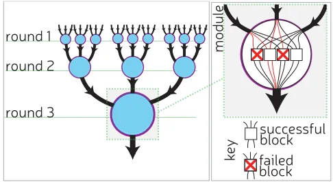
Distillation protocols have many levels forming a treelike structure with many branches that merge at points we call modules, shown in Fig. 2. Branches contain many qubits, which are potentially correlated. However, the inputs to block protocols must not be correlated, so each qubit in a branch must be fed into a different block. Therefore, as we enter a module, a branch of Bl qubits is split up so that each qubit enters a different block. If each block implements anl→kl protocol, then the whole module can be thought of taking
Blnlinputs toBlkloutputs. This entails thatBl+1=Blkland that each module has nl branches feeding into it. Initially, branches are single qubits, B1=1, and so Bl=
[image:4.608.50.293.449.582.2]
1j <lkj.
FIG. 2. The tree structure of many rounds of distillation, with branches (directed black lines) that merge at branching points that we call modules. The thickness of the branch increases with each round. The main plot shows a fictitious scheme wherenl =3 and
kl=2 for all rounds. Inset: The structure within a module. Incoming
branches contain many qubits; here this is shown to be four. These qubits undergo a permutationσand are fed into an instance of a block of a distillation protocol shown as a square. Here the three incoming branches carry four qubits, and so we need four instances of a 3→2 protocol. We use a fictitious protocol to keep the numbers low enough to illustrate clearly. Each of the four blocks output two qubits, and these are merged into a branch of eight qubits fed into a later module. A pernicious error pattern is shown in red (lighter gray), which is detected in two of distillation blocks, marked with crosses, but goes undetected in a third block.
This module-branch structure is common to all proposals to date. Such explicit terminology has not previously been introduced but rather has been left as an implicit consequence of statements about correlation avoidance. Establishing clear vocabulary about this structure is important as we delve into the effect of postselecting at different levels on this structure. Previous protocols have considered whether individual blocks succeed or fail; we call thisblock checking. Below, we outline why it can be advantageous to postselect on the level of the modules, which are collections of blocks. We propose an additional quality check, so that the whole module is discarded whenever any of its blocks fail. We call thismodule checking. A block will always detect a single incoming error but might fail to detect a pair of errors. When a block detects an error, it indicates the presence of damaged branches, and since errors cluster together within branches, this increases the likelihood of errors in other blocks throughout the module. Consider when two branches fail, each with a correlated error pair; the first branch sends damaged qubits to blocks 1 and 2, and the second branch sends damaged qubits to blocks 2 and 3. Since blocks 1 and 3 each received a single erroneous qubit, they will detect them. But block 2 receives a pair of errors, so they may go undetected. A simplified illustration of this process is shown in Fig.2. Module checks improve fidelity by preventing these processes from degrading the output fidelity. Even with module checks, it is possible for a pair of corrupted branches to go undetected, but both branches must carry exactly the same pattern of errors, which is a very rare occurrence.
IV. THEG-MATRIX FORMALISM
Bravyi and Haah introduced a matrix description of their
n→kblock protocols for|T0state distillation. The so-called
Gmatrix is split into two submatrices,G1 andG0, with G0
describing the postselection criteria and G1 accounting for
how input qubits are related to output qubits. For distillation of |T0 magic states, the G matrix must have the property of triorthogonality that the reader can learn about in Ref [16]. Rather, here we give a pragmatic account of the block’s performance. We use|T0 ∝ |0 +eiπ/4|1 for a magic state
and|T1 =Z|T0 for the orthogonal state with aZ error. A
pure multiqubit state|Tx1|Tx2 · · · |Txnwe concisely represent
with the vector x= {x1,x2, . . . ,xn}. If we apply a block protocol to state x, the block succeeds (detecting no errors) ifG0x =0 (mod 2), where the math is performed modulo 2.
When successful, the block outputs a statey =G1x. Noisy
magic states will be some probabilistic ensemble overx, with probability Pr(x). The protocol will detect no errors and output state|Ty1|Ty2 · · · |Tykwith (unnormalized) probability
Prunnorm(y)=
{x:G0x=0,G1x=y}
Pr(x). (2)
The total success probability is captured by the sum over all possible output states, so
Psuc=
y
Prunnorm(y)
=
y
{x:G0x=0,G1x=y}
Pr(x)= {x:G0x=0}
Conditioned on success, the normalized distribution on output states is Prout(y)=Prunnorm(y)/Psuc. Given an explicit form
forG0 andG1, this completes the black box picture of block protocol performance. These formulas form the basis upon which we build both our analytic and numerical analysis in the following sections.
The G-matrix formalism of Bravyi and Haah has been significantly generalized [40,41]. This extension provides protocols that convert noisyTmagic states into another species capable of injecting complex multiqubit circuits. Included in this framework are protocols, based on G matrices, which provide resources for implementing Toffoli gates. Protocols independently proposed by Jones [27] and Eastin [26] realized error-suppressed Toffoli gates, and here we consider a variant based onGmatrices that we discuss further in AppendixE. All three variants perform identically when we use block checking. However, with the G-matrix formalism we can again use module checking to track correlations and achieve superior error suppression. This is just one additional application of module checking; the technique can be deployed in conjunction with the general class of protocols introduced in Refs. [40,41].
V. ANALYSIS OF MODULE CHECKING
We present a method of tracking the leading-order errors, accounting for correlations, through many rounds of module-checked protocols. At each level of distillation the protocol is characterized by a functionηthat summarizes how well it tolerates leading-order errors.
Definition 1. For every distance-2 G-matrix code that distillsn→kqubits, we define a functionη:Zk
2→Z, taking
values
η(y) :=#{y :|x| =2,G0x =0,y =G1x}, (4)
where| · · · |is the weight|y| =jyjand # counts the number of elements in a set{· · · }. In other words, the valueη(y) counts the number of inputsxsuch that (1) they are weight 2 [formally, (|x| =2)], (2) they are undetected by the protocol (formally,
G0x=0), and (3) they giveyas output (formally,G1x=y).
Since η(y) counts the number of lowest-weight errors leading outputy, the total error rate for one round of distillation can be simply estimated as
g =
y
η(y)
2+O(4). (5)
Counting errors over many rounds is a more subtle problem, but we find that η still provides sufficient information to perform this calculation. If each round can even use a different protocol, we label the corresponding function with a subscript. We now state our key result.
Theorem 1.ConsiderLrounds of distillation with module checking, with associated functions η1,η2, . . . ηL. Such a
protocol outputs a multiqubit magic state where thelth-level modules succeed with probability
Psuc,l
Al+Bl (Al−1+Bl−1)nl
(6)
and output states have global infidelity
g(l) Bl Al+Bl
, (7)
where we have made use of the following:
Al=(1−)(n1n2···nl), (8)
Bl =Cl2
l
(1−)(n1n2···nl−2l), (9)
Cl= l
j=1
v
ηj(v)2
l−j
. (10)
The most important quantity in Theorem 1 isCl. After two roundsC2 is simply [yη1(y)2][
yη2(y)]. Afterl rounds,
Clis a product oflterms. One may approximate the theorem to leading order g(l)∼Cl2
l
. However, our later numerical investigations found that such an approximation was too coarse, and we really need the slightly more complex form given in the theorem. We postpone proof of this result to AppendixF.
For the Bravyi-Haah protocols it is easy to verify the following:
ηBHk(y)= ⎧ ⎨ ⎩
3, |y| =2,
4, |y| =k,
0, otherwise,
(11)
so that fork >2 we have
y
ηBHk(y)
m =
4m+3m
k
2
=4m+3mk(k−1) 2 , (12)
where the binomial factor arises in counting the number ofy
where |y| =2. Whenk=2, we have a special case as then the|y| =2 terms and|y| =kterms are the all same, so
y
ηBH2(y)m=7m. (13)
For the Toffoli protocol we have
ηTof(y)=4, y =0, (14)
so
y
ηTof(y)m=7×4m. (15)
Given expressions forη(y)m, we can compose these protocols anyway we wish and obtain an estimate of the global error rate as given in Theorem 1.
We perform numerical Monte Carlo simulations by sam-pling from the probability distribution of the raw magic states, where Pr(x)=|x|(1−)N−|x|, and track its evolution through the magic-state factory.
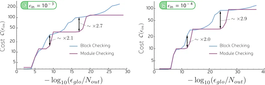
FIG. 3. (a) and (b) The costCof the Bravyi-Haah protocols utilizing both block checking and module checking. It can be seen that only around the transitions to an additional level of distillation is block checking very slightly preferable.
magic-state error rates between 0.1% and 1%. We find that the leading-order analytic estimates match well with the numeric results, with the difference between the two being of the order of a few percent in the investigated parameter regime. In fact, wherever the block protocols are involved, ifk14, we find the percentage difference between the numerical simulation and analytic estimate is<10%. This discrepancy between the analytic estimate and numerical simulations is not visible on log-log plots presented in AppendixG.
The cost of a protocol is the average number of raw magic states consumed to produce one higher-fidelity magic state. For ann→kprotocol, which takes in states with errorp, this is
C(p)= n
kPs(p). (16)
Forlrounds of distillation we haveCl(p)=il−=11Ci(pi). Figure3 compares the cost of a Bravyi-Haah magic-state factory with block checking and module checking, showing the minimum cost achievable for given output error. For output error rate and success probability we use known expressions for block checking, and for module checking we use the success probability and global error given by Theorem 1 with an estimate of the reduced error rate on a single qubit given by the global error rate estimate divided by the total number of qubits in this factory’s output.
We find that module checking is superior to block checking for a large proportion of target error rates and can use up to 4 times fewer raw magic states in some regimes. However, near a transition from j to j +1 rounds of distillation, module checking loses it advantage and may even be slightly outperformed. The best error rates that can be achieved for a given number of rounds use low-k block codes; for these the benefit in the global error rate of module checking over block checking is smaller (see Table II), while the success probability is, of course, much inferior. Above the transition higherkvalues are used, for which the success probability is much lower, and this washes out the benefit of the superior error suppression over block checking, which has a higher success probability. In these regimes, as one might expect, module checking is not the optimal approach. In those regions between the transitions, module checking allows the use of higher-k protocols, which are more efficient, to achieve the error rates of lower-kblock-checked protocols.
VI. FACTORY OVERHEAD ANALYSIS
While the “cost” is a useful guide to the performance of a distillation protocol, it fails to capture several important features of real magic-state factories. The very purpose of magic-state distillation is to supplement the shortcomings of a particular error-correcting code, which is to say that a magic-state factory is implemented at the level of logical qubits, with the quantum information already encoded. As such, the more relevant question is not how many noisy input magic states are required per output state, but rather the number of the physical qubits that will build up such a factory and the rate at which the distilled magic states are produced. Both of these numbers are of key importance to determining the size of a quantum computer and the run time of an algorithm. A single number, the “space-time overhead” of the magic-state factory, captures these both as a figure of merit, which was also studied in Ref. [3]. In this section we present a comparison based on the space-time overhead of implementing a magic-state factory in a surface code quantum computer, utilizing module checking, where appropriate, and our implementations of the Reed-Muller, Bravyi-Haah, and Toffoli protocols.
We consider a number of issues in this estimate of the footprint of a magic-state factory, including (1) balanced investment, the use of smaller surface codes during early rounds of magic-state distillation, and (2)clock-rate zoning, cycling through distillation attempts faster during early rounds of magic-state distillation. We will assume throughout that we use the method outlined by Li [42] to inject the initial raw magic state into a logical surface code. We will therefore assume throughout that the initial error rate on a magic state before distillation is in=0.4pg. We also use the
“rotated-lattice” surface codes [29], such that a distance d surface requiresd2physical data qubits. Of course a practical surface code requires the use of physical ancilla qubits to make the stabilizer measurements of the code; we leave this as an extra multiplicative factor to be applied to our overhead calculated here, as different physical realizations have different requirements. We estimate the surface code distance required to protect a logical qubit up to error ratePlusing the relation
Pl(d,pg)=d(100pg)
d+1 2 [3].
[image:6.608.88.517.70.208.2]TABLE II. The leading coefficientClfor a variety of protocols with two and three levels of distillation. For clarity we also showClin the
large block limit (k→ ∞). When we write BHk, we implicitly assumek >2, as the results differ slightly for thek=2 case. The final column
shows the ratio between the union bound estimate made by utilizing the reduced error rate on a single qubitBHmade by Bravyi and Haah and
the corresponding estimate of the global error rate given byCl2 l
. It can be seen that the benefit (in error rate) of module checking scales with bothkand the number of rounds of distillation.
Level 1 Level 2 Cl limk→∞Cl limk→∞k1k2BH/4
BHk1 BHk2
16+ 9
2k1(k1−1)
4+ 3
2k2(k2−1)
27
4k 2 1k
2
2 27k
3 1k
2 2
Tof BHk 112
4+ 3
2k(k−1)
168k2 2352k2
BHk Tof
16+9
2k(k−1)
28 126k2 252k3
Level 1 Level 2 Level 3 Cl limk→∞Cl limk→∞k1k2k3BH/8
BHk1 BHk2 BHk3
256+81
2k1(k1−1)
16+9
2k2(k2−1)
4+3
2k3(k3−1)
273.375k2 1k
2 2k
2
3 2187k
5 1k
3 2k
2 3
Tof BHk1 BHk2 1792
16+9
2k1(k1−1)
4+3
2k2(k2−1)
12096k2 1k
2
2 28
4×33k3 1k
2 2
BHk1 BHk2 Tof
256+81
2k1(k1−1)
16+9
2k2(k2−1)
28 5013k2
1k 2
2 20412k
5 1k
3 2
its magic-state factory is capable of producing magic states of fidelity great enough that there is a high probability that none of the magic states required for the algorithm fail. Thus, we set a target global error rate that our factory must achieve:
target=1−(Psuc,alg)1/N, (17)
where Psuc,alg is the desired success probability of our
algorithm (i.e., the probability that every non-Clifford gate works) andN is the number of successful iterations of the factory needed to produce the desired number of magic states. For example, a magic-state factory which utilizes three rounds of Bravyi-Haah distillation with akvalue of 10 in each round will produce 1015 |T states after 1012 successful iterations.
A 90% success probability for the algorithm as a whole then implies target=1.05×10⁻¹³. We must then check that the
factory is capable of producing an output of this quality. If the factory is module checked, then this “10-10-10” factory has a global error rateglo =2.3×10⁻¹⁶, making this a valid
protocol. However, the estimate of the global error rate of a block-checked factory gives 103×
BC ∼10−11, so this would not be a valid factory for this task.
A. Balanced investment
Once we have established that a factory is valid, we can calculate the space-time overhead per magic state that it produces. This is done by calculating the distance of surface code required at each level of distillation di, the length of time in surface code cycles that each round of distillation will takeTi, and the number of logical qubitsQi, including logical ancillas, required at each level of the factory.
Determining the distance required at each level requires slightly different methods depending on whether module or block checking is used. To obtain the benefits of module checking we cannot make full use of balanced investment at the lower levels because doing so would inject noise at a rate comparable to or greater than the rate of correlated error. We can estimate the total global error output in the output of an→kprotocol astot∼glo+kenc, whereenc
is the random error rate resulting from the size of the logical encoding chosen. As such we determine the distance of the code at the intermediate levels based on a desired error rate
encto be 0.1glo/kto ensure that the error due to each qubit’s
finite encoding is much less than the reduced error∼glo/kon that qubit. The final output of the factory can then ne encoded according totarget.
For a block-checked factory (or the original 15-to-1 Reed-Muller protocol) we do not have worry about “protecting” correlated errors. This means we can work backwards from our error target to determine an efficient balanced investment of qubits, as illustrated in Fig. 4. For a local target error of
ptop=10−14the top level of distillation needsvPL(d,enc)<
0.1×10⁻¹⁴, where v is the space-time volume of a single
block of distillation, which is the number of surface code qubits in the block multiplied by the number of times they undergo
d rounds of surface code stabilizer measurements. Again, we use a distance corresponding to a lower error rate by a factor of 10 to suppress any error injected by the logical circuitry above that which is left over after distillation. The distance required for the next level down can then be determined by, in this example, pi−1= 3
ptop/35 for the 15-to-1 protocol, which gives distancedi−1, and so on untilpi > pin.
[image:7.608.336.533.530.670.2]FIG. 5. Space-time overheads of producing both (a) and (b)|Tstates and (c) and (d)|Toffstates. Note that module checking is more beneficial when one of the rounds of distillation is Toffoli.
The length of timeTi for each round of distillation can be simply determined by the protocol used and how many times we attempt it before abandoning the round. We assume that measurements can be completed in one time step, and the time scale of theCNOTgates, preparation, andAgates is dominated by the requirement for d rounds of stabilization afterwards. Therefore, we let the time for each of these bed×tsc. The time taken to implement the distillation protocol in roundiis then
τi=
⎧ ⎨ ⎩
11tsc×d, roundiuses Bravyi-Haah,
12tsc×d, roundiuses Toffoli,
13tsc×d, roundiuses Reed-Muller.
(18)
B. Clock-rate zoning
Balanced investment also allows another advantage. In the context of surface code computing, the distance of the code is relevant for not only the spatial dimensions of the computer but also the execution time. A surface code of distance d
must undergod rounds of parallel stabilizer measurements to protect from measurement errors. As such, the time taken for a logical operation is proportional to d (except those which can be handled in software), and therefore, using balanced investment, the initial rounds of distillation will take less time. In the hypothetical case that a round of distillation leads to a squaring of the input error rate, this would correspond to a doubling of the code distance required by the next round (by the exponential suppression of error with distance of a subthreshold surface code). Therefore, one can repeat the first round of distillation twice in the time taken for the second round of distillation to be completed. This increases the chance that all the necessary magic states for the second round will have been produced in time for the next round of distillation,
without the need to decrease the rate of the factory. As such, the time taken for a round to complete in the distillation factory isTi =τiti, wheretiis the number of attempts that you allow at each round. In all our simulations, any “idle time” that the qubits experience is counted towards the space-time cost.
C. Numerical simulations
We have therefore arrived at the expression for the full space-time volumeVin qubit rounds occupied by a factory,
V(in,pg,N,{ki},{ti},Psuc,alg)
=
r
i=1QiTidi2
r
ikiPsuc,i
=
r
i=1Qiτitidi3
r
ikiPsuc,i
, (19)
where ki labels the magic-state protocol used at each round and Pi is the probability that round i of distillation will succeed in producing enough magic states to feed the next round. All rounds must succeed for the factory to successfully output riki magic states. As discussed,V is a function of several variables, the raw magic-state error ratein, the error
of gate operationspg, the total states requiredN, the protocol
chosen {ki}, the repetitions allowed in each round {ti}, and the probability with which you wish the algorithm to succeed
Psuc,alg.
In practice we calculateV for one, two, and three rounds of distillation using combinations of the Bravyi-Haah, Reed-Muller, and Toffoli protocols with our proposed implementa-tions, with both block and module checking, and a variety of combinations of ti. We then search for the most space-time efficient method of producing eitherT or Toffoli magic states, given apg, assumingin=0.4pg, the number of magic states
Figure 5 shows the results of these simulations which suggest that module checking can provide an improvement of a factor of 3 in the space-time overhead in certain parameter regimes. We also see that in some regions module checking can be detrimental by a small amount, such as near the transition fromitoi+1 rounds of Bravyi-Haah.
[image:9.608.49.296.238.549.2]We use the numbers we have generated to estimate the size of a magic-state factory required to perform some postclassical factoring tasks using Shor’s algorithm. Our results are summarized in TableII, in which we approximate Shor’s algorithm as modular exponentiation, as this is by
FIG. 6. To produceT magic states at a “time-optimal” rate the factory must, on average, produce states at a rate equal to the fastest rate at which they can be used in sequence by an algorithm. In this paper, where we have assumed thattsc=10tmeas/ff, this means ten
magic states must be produced on average everytscto keep up with
the time-optimal implementation of the algorithm. As this figure makes clear, it is indeed possible to produce a given number of magic states faster (slower) than this using more (fewer) qubits. Each data point represents one possible magic-state factory given the input error and target number of 1016T magic states; only the factories near the
boundary between possible and impossible factories are shown. Not shown in the lower right of each graph are myriad other possible factories of lower rate and higher overhead. As seen clearly in (a), doubling the size of the factory can allow one to more than double the rate of magic-state production when the larger factory allows the use of the higher-k(and therefore higher-rate) block codes. This point is less evident in (b), where only two rounds of distillation can be sufficient and the higher-kblock codes are not necessarily optimal.
far its most expensive part, and choose the minimum Toffoli gate-count implementation, which has Toffoli count and depth equal to 40N3 for anN bit number [43]. We then determine
the minimum possible space-time overhead per magic state for this task and also the smallest possible factory, in terms of physical qubits, that can produce all the magic states necessary while keeping up with a time-optimal quantum computation [14].
The smallest possible factory is not necessarily the most space-time efficient factory possible: these factories tend to use larger k blocks which can make the factory formidably vast (see Fig.2) but able to produce more qubits in the same time as lower-kprotocols. However, these may well produce magic states much faster than required by the fastest possible implementation of the algorithm. Figure 6 shows that it is possible to use fewer qubits than required by the time-optimal implementation and perform your computation at a reduced speed. Equally, it is, of course, possible to increase the size of the factory to produce magic states at a faster rate. In this case, though, the extra qubit overhead is effectively wasted unless the computer is performing many calculations in parallel. We find that all the magic states required for a time-optimal factorization of a 1000-bit number can be produced with a surface code magic-state factory of 5.6 million “data qubits” if the infidelity of operations on physical qubits is 10−4. This is
based on the cost ofd2physical qubits to store the information in the rotated lattice surface code [29]. However, for many architectures this number must be doubled to provide ancillas responsible for syndrome extraction. In this case the physical qubit overhead would be∼11 million.
[image:9.608.314.557.518.669.2]A summary of the time and space overheads for some example Shor tasks can be found in Table I. We selected Shor’s algorithm as a benchmark as the number of non-Clifford gates required has been well studied and these results have been used in previous analyses. We note that due to the large resource overhead that we have demonstrated, early quantum computers may focus on other problems, particularly in
FIG. 7. The scaling of resource cost in qubit rounds per magic state is not worse than that of the surface code. This corroborates the predictions of Raussendorfet al.[28] and suggests that the asymptotic overhead scaling∼O(log(N)3)of the surface code is applicable to
quantum chemistry. A recent analysis of some such problems [44] demonstrates that they are solvable with overheads lower than we find here, albeit that work makes more optimistic assumptions of gate times and fidelities.
Of significant interest is how the cost of magic-state dis-tillation compares to the surface code overhead. Raussendorf et al. (see Sec. 6.2 of Ref. [28]) were the first to note that using balanced investment in a magic-state distillation leads to a constant factor overhead compared to theCNOTgate. Our numerical results in Fig.7show a ratio betweenT-gate cost and CNOTcost in the range of∼150–310 when 1010 < N <1030. This ratio is much smaller than estimated by Raussendorfet al., who did not make use of Bravyi-Haah distillation routines. A similar ratio can be extracted from the data tables provided in Ref. [3], although the numbers are not directly comparable. For instance, we also count the space-time volume due to idle qubits, while they wait for distillation circuits to succeed.
VII. CONCLUSIONS
We proposed the notion of gauge-MSD, which is faster and uses fewer ancillas than previous realizations of Bravyi-Haah magic-state distillation. We further introduced module checking as a means to exploit correlations and found it gave an additional factor of∼3 reduction in some parameter regimes. Fowler et al.[3] considered realizing Bravyi-Haah using braiding and found that Bravyi-Haah offered only a modest factor ∼3 improvement over the first magic-state proposal that used Reed-Muller codes [1]. Therefore, our gains are comparable to, and build upon, other advances in the field. The work of Bravyi and Haah predicted a much greater improvement because they quantified cost by the expected conversion efficiency of raw to high-fidelity magic states. In a fully costed analysis, which we perform here, error correction costs overwhelm and dominate the cost of magic-state factories. We saw that an efficiently designed factory using balanced investment is entirely limited by the surface code cost, so refinement in distillation protocols can offer only constant factor improvements.
It is likely that this analysis represents an overestimate of the space-time overhead of the implementations of the distillation circuits we describe. We have assumed the need fordrounds of surface code measurements after every two-qubit gate. However, it is not clear that this is necessary when performing transversal gates. In the implementation of Bravyi-Haah (see Fig. 1) it may prove feasible to perform d rounds of error correction only after, say, the completion of each of the four steps described, reducing the time overhead from 11tscd
to 4tscd [45]. Our cost analysis here could thus be further developed by considering the effect on the performance of the underlying surface code if multiple transversal operations were performed between rounds of error correction. However, such simulations lie beyond the scope of this paper.
Three-dimensional (3D) gauge color codes [7,25] and other recent ideas do not require magic states. But they have their own hidden costs. For 3D gauge color codes, spatial overheads scale as ∼O(log(N)3), and time overhead scales
as O(1). Using balanced investment and surface codes, we see similar asymptotic scaling of resources. However, current evidence indicates an order of magnitude worse phenomeno-logical threshold for color codes [11,12] compared to the
phenomenological threshold for the surface code. Although a full circuit-based threshold has not yet been determined, it is unlikely to challenge that of the surface code due to the higher weight stabilizers required. This points towards 3D color codes requiring physical error rates below 0.1%. Resource costs are heavily influenced by proximity to threshold, so 3D color codes seem to require significantly lower physical error rates before they can start to compete with surface codes augmented by magic states. Therefore, with current technology and fidelities, known schemes for avoiding magic states are a false economy. An additional benefit of the magic-state paradigm is that it can also eliminate the additional burden of gate-synthesis costs by preparing exotic magic states [40,41,46–49].
ACKNOWLEDGMENTS
E.C. is supported by the EPSRC (Grant No. EP/M024261/1). We thank M. Howard for comments on the manuscript. We acknowledge support from the EPSRC National Quantum Technology Hub in Networked Quantum Information Technologies in facilitating this collaboration. The authors would like to acknowledge the use of the University of Oxford Advanced Research Computing (ARC) facility in carrying out this work.
APPENDIX A: COMPARISON WITH BRAIDING Here we discuss how our results compare with prior work on braiding defects in the surface code. It has been shown that Bravyi-Haah can be realized in constant time [3] assuming the architecture supports constant time implementations of multitargetCNOTgates (in timetMT−cnot). This has time cost
tblock(2) =12tMT−cnot+tA+tprep+tinject+tmeasure, (A1)
wheretinjectis the time to inject a magic state into the circuit
and we can infertinject=tcnot+tmeasure.
In the standard circuit model, multitargetCNOTgates do not take constant time to implement. In the braiding picture, using ancillary defects, this is possible. The “time” cost of braiding 12 such gates is 12×1.25×d×tsc. The total space-time cost was reported as (96k+216) so-called plumbing pieces, which converts into (54)3(96k+216) qubit rounds. It has recently
been shown that lattice surgery also supports multitargetCNOT gates in constant time [50]. Although the Bravyi-Haah protocol was not considered in this setting, one can infer a lattice surgery time cost also scaling with ∼12d, but the qubit cost is not currently known.
The above discussion implies a modest space-time saving of using gauge-MSD in a distributed architecture rather than braiding in a nearest-neighbor picture. We remark that gate times and qubit expense will vary on a much greater scale between different hardware platforms. In particular, the long-range gates of distributed schemes are often much slower, with photonic protocols impeded by photon loss and the potential need for entanglement purification [31–38].
APPENDIX B: FORMAL TOOLS 1. Stabilizer Bravyi-Haah codes
by an Abelian group called the stabilizer S, which is a subgroup of the Pauli group. The projector onto the code space is∝s∈Ss, so thats= for alls∈S. There always exists a minimal set of operators {S1,S2,...Sm} that generates the group, which we denote byS= S1,S2, . . . ,Sm. For the Calderbank-Shor-Steane (CSS) codes, these generators can be chosen so that they are all either X type or Z
type, as we define shortly. If g is a binary vector of lengthn, we use Z[g]= ⊗n
j:[g]j=1Zj and, similarly,X[g]=
⊗n
j:[g]j=1Xj. We sayZ[g] areZ-type operators andX[g] are X-type operators. Therefore, a CSS code has generatorsS =
Z[f1], . . . ,Z[fa],X[g1], . . . ,X[gb]. Commutation ofX[g]
andZ[f] is equivalent to (f,g)=0, where we use the inner product (f,g) :=f g (mod 2).
Bravyi and Haah introduced the notion of a G matrix which is a binary matrix composed of two submatrices,G1
andG0. We label the rows ofGas{g1, . . . ,gb,gb+1, . . . gm}, where the rows {g1, . . . ,gb} belong to G0 and the rows
{gb+1, . . . ,gm}belong to G1. These matrices define a CSS
code as follows. The rows ofG0 are some set {g1, . . . ,gb} that specifies theX-type generators{X[g1], . . . ,X[gb]}. The
Z-type generators are given less explicitly. Denote G⊥ as the binary vector space orthogonal to bothG0 andG1, that
is,G⊥:= {g: (f,g)=0;∀f ∈G0,G1}. Note that Bravyi and Haah required thatG0⊂G⊥. We defineG⊥as some (minimal) matrix with rows {f1, . . . ,fa} that generate the group G⊥ under row-wise modular addition. This defines the Z-type generators {Z[f1], . . . ,Z[fb]}. Note that there exist many
different choices forG⊥, which all result in the same CSS code withZ-type generators{Z[f1], . . . ,Z[fa]}.
This completes the description of the stabilizer code space, although we also need to know how information is stored within the subspace. We have that theXoperator for thekth logical qubit isX[gk], wheregk is a row ofG1, sob+1
km. These are representatives of the logical operators, with equivalent logical operators differing by only a stabilizer. For Bravyi-Haah protocols all rows inG1have odd weight, so we
may also take theZoperator for thekth logical qubit asZ[gk], wheregkis thekth row ofG1.
2. Subsystem Bravyi-Haah codes
Given a G matrix, we define a subsystem code with stabilizer ˜S := Z[g1], . . . ,Z[gb],X[g1], . . . ,X[gb], where
{g1, . . . ,gb}are the rows ofG0. Notice that now there are equal
numbers ofX andZ stabilizers, and they both correspond to the rows ofG0. Bravyi and Haah considered a class of matrices obeying triorthogonality conditions, which require thatG0⊂
G⊥. Therefore, we have that ˜S ⊂S, with the subsystem code having strictly fewer stabilizers than the original Bravyi-Haah code. We denote the subsystem projector as ˜∝s∈S˜s.
We further take the logical operator for the subsystem code to be identical to those of the original Bravyi-Haah code. This leaves some degrees of freedom as neither stabilizers nor logical operators. We define the gauge group Sg :=
Z[f1], . . . ,Z[fa],X[f1], . . . ,X[fa], where {f1, . . . fa} are rows of G⊥. Notice that Sg contains S by virtue of
G0⊂G⊥.
Let us recap. Our subsystem code is defined by its stabilizer ˜
S and gauge group Sg, whereas the original Bravyi-Haah
code has stabilizerS, and these groups satisfy ˜S ⊂S ⊂Sg. However,Sgis inflated in size compared toSand is no longer Abelian. Furthermore, one can verify thatSgdoes not contain any logical operators as follows. First, note that Bravyi and Haah use triorthogonal (also called triply even) matrices where for anyf,g∈Gwe have (f,g)=1 if and only iff =gand
f ∈G1.
As logical operators we takeX[l] andZ[l] for eachl in
G1. From the triorthogonality of G we see that X[l] and
Z[l] anticommute, butX[l] andZ[l] commute whenl =l. To properly describe a subsystem code, where measuring the gauge operators does not damage the logical qubits, we require that the logical operators are not elements of the gauge group Sg. Recall that the gauge group is defined by vectors that reside in the dual code G⊥. Therefore, every gauge operator must have a vanishing inner product with every row inG. However,
l∈G, and (l,l)=1, so l is not in the dual space, and the logical operators are not gauge operators. This completes our proof that the logical operators indeed lie outside the gauge group.
APPENDIX C: REALIZING THE BRAVYI-HAAH PROTOCOLS
There are many routes to realizing magic-state distillation. Assuming perfect Clifford operations, different realizations suppress errors equally but differ in terms of temporal depth and required ancillas. Many of these potential realizations have only been sketched, without a complete assessment of resources involved. Here we introduce a method particularly suitable for architectures implementing logical gates via transversal operations or lattice surgery [29]. Conceptually, we are inspired by notions of subsystem codes and gauge-fixing techniques and so call our approach gauge-MSD. We consider only evenkwithk∈ {2,6, . . . ,4m+2, . . .}as then the Bravyi-Haah codes have transversal T gates. For k∈ {0,4,8, . . . ,4m, . . .}, the Bravyi-Haah codes have transversal
T gates only up to a nonlocal Clifford correction.
1. Outline of protocol
Here we present an outline of gauge-MSD, with details of how to realize multiqubit Pauli measurements postponed until the next section. First, we specify some notation. Refer back to AppendixBfor definitions of theGmatrix andG⊥matrix. Let
R be a binary matrix such thatG⊥·R=1l (mod 2), which is ensured to exist by virtue of the fact thatG⊥ is full rank. Furthermore, letMbe a binary matrix such thatM·G⊥=G0
(mod 2), which must exist since G0 is in the span ofG⊥.
Explicit examples ofG⊥,R, andMwill be given in the next section. Measurement outcomes will be recorded in binary: 0 for+1 eigenvalues and 1 for−1 eigenvalues. LetO,X, and Zbe disjoint sets:
O= {6+3j|j =1,2, . . . k},
X = {1,2,3},
Z = {4,5,6,7,8,7+3j,8+3j|j =1,2, . . . ,k}. (C1)
ak-by-|Z|matrix as follows:
4 5 6 7 8 10 11 13 14 16 17 . . .
HZ=
⎛ ⎜ ⎜ ⎝
0 1 1 1 1 1 1 0 0 0 0
0 1 1 1 1 0 0 1 1 0 0 . . .
0 1 1 1 1 0 0 0 0 1 1
..
. ...
⎞ ⎟ ⎟
⎠(C2)
1 2 3
HX =
⎛ ⎜ ⎜ ⎝
1 1 0
1 1 0
1 1 0
.. .
⎞ ⎟ ⎟
⎠ (C3)
where the numbers above the columns correspond to the elements in sets Z and X. Last, we will also make use of a k-by-dim(G⊥) matrix denoted Q that satisfies G1=
W+QG⊥, whereWhasWj,6j+3=1,Wj,1=Wj,2=1 and
is zero everywhere else. An example Qis given in the next section.
We now state the protocol:
(1) Measure all Z[fk], where fk is the kth row ofG⊥, recording outcomes asμ=(μ1,μ2, . . . ,μk).
(2) ApplyA[w], wherew=Rμ (mod 2).
(3) Measure all X[fk], where fk is the kth row of G⊥, recording the outcome asγ =(γ1,γ2, . . . ,γk).
(4) Declare success ifMγ =(0, . . . ,0) (mod 2) and failure otherwise.
(5) Measure qubits in set X in the X basis, recording outcomes as mX. Simultaneously, measure qubits in set Z in theZbasis, recording outcomes asmZ.
(6) Qubits inX andZare discarded, while qubits in setO are retained as output as qubits (1,2, . . . ,k).
(7) Apply Pauli correctionsX[HZmZ]Z[HXmX+Qγ], or update the Pauli frame accordingly.
After steps 1 and 2, the state is deterministically projected by Z ∝
s∈SZs, whereSZ := Z[f1], . . . ,Z[fa], exactly
as in the original Bravyi-Haah protocol. After step 3, the system is an eigenstate of (−1)γkX[fk], and we can associate
some projector withX,γwith this process. The postselection in step 4 ensures the system is an eigenstate of+X[gk], where
gk is the kth row of M·G⊥. Since we definedM such that
M·G⊥=G0, we have thatgkare the rows ofG0. It follows
that X,γ =XX,γ, whereX is the projector for theX stabilizer of the Bravyi-Haah stabilizer code. Combining steps 1–4, we have the projections
X,γZ =X,γXZ=X,γ, (C4)
where=XZis the full projector onto the Bravyi-Haah stabilizer code space.
We have obtained the desiredprojection required by the Bravyi-Haah protocol. But we have picked up an additional
X,γ. This additional projection results from measuring some gauge operators of the subsystem variant of Bravyi-Haah. Thus, the logically encoded qubits are unharmed, but there has been a change in the gauge degrees of freedom.
In step 5, we perform single-qubit measurements to isolate theklogical qubits from thenqubits in the subsystem code. Recall that in the original presentation of Bravyi-Haah we have logical operators Z[lj] and X[lj] for the jth logical qubit, where lj is the jth row of G1. The measurements
localize these logical operators onto single qubits, up to a Pauli correction depending on the measurement outcomes. That is, the measurements cause the state to become stabilized by some new±Z[w] operators, and every logicalZ[lj] can be multiplied by these operators to obtain a single-qubit±Z
operator acting on the (6+3j)th qubit. It is straightforward to verify that the±sign is corrected to+by the Pauli correction
X[HZmZ]. To show thatXlogical operators are also localized on a single output qubit, we first multiplyX[lj] byX-type gauge operators until it acts on qubits 2, 3, and (6+3j). Measuring qubits 1, 2, and 3 completes the localization of
X[lj] onto the (6+3j)th qubit. The required Pauli operator is nowX[HZmZ+Qγ], where there is also some dependence on the eigenvalues of gauge operators obtained in step 3.
2. Implementing Pauli measurements in minimum depth Implementing the protocol requires a set of Z measure-ments, followed by a set ofXmeasurements. In the original standard implementation theXmeasurements involved many qubits and so were difficult to implement. However, the previous section shows that the difficult X measurements can be replaced with lower-weight measurements mirroring the Z measurements performed. The complexity of these measurements depends on the row weights ofG⊥. The matrix
G⊥ must generate the space G⊥, but there is some freedom in how we choose the generating rows. In the work of Bravyi-Haah,G⊥was only implicitly defined (as the dual of
G), leaving unclear how much time it would take to implement the required measurements. It is desirable thatG⊥is as sparse as possible to minimize the resource overheads. Therefore, we wish to find a very sparseG⊥. We found a family ofG⊥
matrices where all rows, except one, are weight 4 and the single exception has weightk+2. We present the exact form of thisG⊥fork=2, along with the associatedR,M, andQ
matrices used in the previous section:
G⊥ =
⎛ ⎜ ⎜ ⎜ ⎜ ⎜ ⎜ ⎜ ⎜ ⎜ ⎜ ⎜ ⎝
1 0 0 1 0 1 1 0 0 0 0 0 0 0
0 1 0 1 1 0 1 0 0 0 0 0 0 0
0 0 1 1 1 1 0 0 0 0 0 0 0 0
0 0 0 0 1 0 0 1 1 1 0 0 0 0
0 0 0 0 0 1 0 1 1 0 1 0 0 0
0 0 0 0 0 0 1 1 0 1 1 0 0 0
0 0 0 0 0 0 0 0 1 1 0 1 1 0
0 0 0 0 0 0 0 0 0 1 1 0 1 1
0 0 1 0 0 0 1 0 1 0 0 1 0 0
⎞ ⎟ ⎟ ⎟ ⎟ ⎟ ⎟ ⎟ ⎟ ⎟ ⎟ ⎟ ⎠
R= ⎛ ⎜ ⎜ ⎜ ⎜ ⎜ ⎜ ⎜ ⎜ ⎜ ⎜ ⎜ ⎜ ⎜ ⎜ ⎜ ⎜ ⎜ ⎜ ⎜ ⎜ ⎝
1 0 0 0 1 1 0 0 0
0 1 0 1 0 1 0 0 0
0 0 1 1 1 0 0 0 0
0 0 0 0 0 0 0 0 0
0 0 0 1 0 0 0 0 0
0 0 0 0 1 0 0 0 0
0 0 0 0 0 1 0 0 0
0 0 0 0 0 0 0 0 0
0 0 0 0 0 0 0 0 0
0 0 0 0 0 0 0 0 0
0 0 0 0 0 0 0 0 0
0 0 1 1 1 1 0 0 1
0 0 1 1 1 1 1 0 1
0 0 1 1 1 1 1 1 1
⎞ ⎟ ⎟ ⎟ ⎟ ⎟ ⎟ ⎟ ⎟ ⎟ ⎟ ⎟ ⎟ ⎟ ⎟ ⎟ ⎟ ⎟ ⎟ ⎟ ⎟ ⎠
, Q=
1 1 0 0 0 1 0 0 0
1 1 0 0 0 1 0 1 0
,
M=
⎛
⎝00 10 01 11 11 11 01 11 00
1 1 1 1 1 1 0 0 0
⎞ ⎠.
AMathematicascript for generatingG⊥for anykis provided in the Supplemental Material [51], which also verifies thatG⊥
is full rank and dual toG. As one further example, we find fork=6 that
G⊥=
⎛ ⎜ ⎜ ⎜ ⎜ ⎜ ⎜ ⎜ ⎜ ⎜ ⎜ ⎜ ⎜ ⎜ ⎜ ⎜ ⎜ ⎜ ⎜ ⎜ ⎜ ⎜ ⎜ ⎜ ⎜ ⎜ ⎜ ⎝
1 0 0 1 0 1 1 0 0 0 0 0 0 0 0 0 0 0 0 0 0 0 0 0 0 0
0 1 0 1 1 0 1 0 0 0 0 0 0 0 0 0 0 0 0 0 0 0 0 0 0 0
0 0 1 1 1 1 0 0 0 0 0 0 0 0 0 0 0 0 0 0 0 0 0 0 0 0
0 0 0 0 1 0 0 1 1 1 0 0 0 0 0 0 0 0 0 0 0 0 0 0 0 0
0 0 0 0 0 1 0 1 1 0 1 0 0 0 0 0 0 0 0 0 0 0 0 0 0 0
0 0 0 0 0 0 1 1 0 1 1 0 0 0 0 0 0 0 0 0 0 0 0 0 0 0
0 0 0 0 0 0 0 0 1 1 0 1 1 0 0 0 0 0 0 0 0 0 0 0 0 0
0 0 0 0 0 0 0 0 0 1 1 0 1 1 0 0 0 0 0 0 0 0 0 0 0 0
0 0 0 0 0 0 0 0 0 0 0 1 1 0 1 1 0 0 0 0 0 0 0 0 0 0
0 0 0 0 0 0 0 0 0 0 0 0 1 1 0 1 1 0 0 0 0 0 0 0 0 0
0 0 0 0 0 0 0 0 0 0 0 0 0 0 1 1 0 1 1 0 0 0 0 0 0 0
0 0 0 0 0 0 0 0 0 0 0 0 0 0 0 1 1 0 1 1 0 0 0 0 0 0
0 0 0 0 0 0 0 0 0 0 0 0 0 0 0 0 0 1 1 0 1 1 0 0 0 0
0 0 0 0 0 0 0 0 0 0 0 0 0 0 0 0 0 0 1 1 0 1 1 0 0 0
0 0 0 0 0 0 0 0 0 0 0 0 0 0 0 0 0 0 0 0 1 1 0 1 1 0
0 0 0 0 0 0 0 0 0 0 0 0 0 0 0 0 0 0 0 0 0 1 1 0 1 1
0 0 1 0 0 0 1 0 1 0 0 1 0 0 1 0 0 1 0 0 1 0 0 1 0 0
⎞ ⎟ ⎟ ⎟ ⎟ ⎟ ⎟ ⎟ ⎟ ⎟ ⎟ ⎟ ⎟ ⎟ ⎟ ⎟ ⎟ ⎟ ⎟ ⎟ ⎟ ⎟ ⎟ ⎟ ⎟ ⎟ ⎟ ⎠ .(C6)
Notice that the bottom row has weight exceeding 4. The measurements corresponding to weight-4 rows can be im-plemented with each measurement using a single ancilla in the|+state and four entangling gates (controlZ or control
X depending on the measurements). Therefore, for these measurements it is possible that all these gates can be realized in four time steps while respecting that a qubit can be involved in only a single entangling gate at a time. Unfortunately, there is a single row of G⊥ with weight k+2, so using a single ancilla to perform this measurement would result in a growing time cost with k. Therefore, for this single measurement we make use of a cat state|0⊗k+2+ |1⊗k+2
so that the entangling gates can be performed in parallel. The cat state itself is constructed by merge operators on|+⊗k+2
qubits. The merge operations project onto|0000| + |1111| or |0101| + |1010| subspaces and so commute with the control gates, so the cat state can be built concurrently with the control gates. This opens the possibility of realizing each round of measurements in four times steps but depends
on whether the entangling gates can be scheduled in an economical manner. The scheduling problem is equivalent to a graph coloring problem, and we find that it can be solved in four time steps (e.g., using four colors) as in Fig. 1. We independently confirmed this using an automated solver of the edge colorability problem forkup to 40; see supplementary Mathematicascript for details.
APPENDIX D: REED-MULLER CONNECTIVITY The usual form of the 15-qubit punctured Reed-Muller code
Gmatrix is
GRM =
⎛ ⎜ ⎜ ⎜ ⎝
1 1 1 1 1 1 1 1 0 0 0 0 0 0 0 1 1 1 1 0 0 0 0 1 1 1 1 0 0 0 1 1 0 0 1 1 0 0 1 1 0 0 1 1 0 1 0 1 0 1 0 1 0 1 0 1 0 1 0 1 1 1 1 1 1 1 1 1 1 1 1 1 1 1 1