unsupervised learning of finite mixture
models with deterministic annealing for
large-scale data analysis
jong youl choi
Submitted to the faculty of the University Graduate School in partial fulfillment of the requirements
for the degree Doctor of Philosophy
in the School of Informatics and Computing Indiana University
Accepted by the Graduate Faculty, Indiana University, in partial fulfillment of the
require-ments for the degree of Doctor of Philosophy.
Doctoral Committee
Geoffrey Fox, Ph.D.
Paul Purdom, Ph.D.
David Wild, Ph.D.
Sun Kim, Ph.D.
Jong Youl Choi: Unsupervised Learning Of Finite Mixture Models With Deterministic
Anneal-ing For Large-scale Data Analysis,Thesis, © January2012.
website:
http://www.cs.indiana.edu/~jychoi/
e-mail:
D E D I C A T I O N
This thesis is dedicated to my lovely wife, Hyejong Jang, who always endures everything
with me and gives endless love and encouragement
A C K N O W L E D G E M E N T S
I would like to express my sincere gratitude to my advisor, Professor Geoffrey Fox, for
his support and guidance of my research and his endless patience. Without his help, it
would be impossible to write this thesis. I am extremely fortunate to have him as my
advisor.
I also would like to thank my research committee: Professor Paul Purdom, Professor
Sun Kim, and Professor David Wild, for valuable discussions and insightful comments.
I am very grateful to have been a Ph.D. student in the School of Informatics and
Com-puting where I could enjoy intellectual conversations and interactions with bright many
professors and researchers.
My sincere thanks also goes to Professor Judy Qiu for her help and guidance on projects
I worked with and new challenges that inspired me. I am indebted to my previous
advisor, Dr. Markus Jakobsson, who gave me a great opportunity to start my Ph.D. study
and provided countless help and advice.
I would like to thank my friend, Youngsang Shin, who didn’t hesitate to give invaluable
advice and immense help on my researches and life in Bloomington. I also thank to my
fellow, Seung-Hee Bae, a fantastic collaborator and a lab mate to discuss many things
on research. I wish to express my thanks to my lab fellows Thilina Gunarathne, Yang
Ruan, Saliya Ekanayake, Hui Li, Tak-Lon Wu, Yuduo Zhou, and Bingjing Zhang for their
collaboration and comments for my research.
I would like to give my special thank to my wife, Hyejong Jang, for everything during
my study. My sincere thanks goes to my parents, who gave everything and support me
always. Last but not the least, I would like to extend my thanks to my parents-in-law for
generous support and encouragement.
A B S T R A C T
The finite mixture model forms one of the most fundamental foundations in the fields of
statistical pattern recognition, data mining, and machine learning to access the essential
structure of observed random sample data. It aims at building a probabilistic generative
model by which one can virtually reproduce the observed sample data from a mixture
of a finite number of probabilistic distributions calledlatentcomponents or sources. The
finite mixture model provides a flexible and convenient way to explain a wide variety
of random phenomena of observed sample data in a generative process of mixing finite
random sources.
One of the main challenges in the finite mixture model is to search an optimal model
parameter set from a large parameter space. The standard method used to fit a finite
mix-ture model is the Expectation-Maximization (EM) algorithm. However, theEMalgorithm
for finite mixture model has a serious drawback; it can find only local optimum solutions
and thus the quality of answer can be heavily affected by initial conditions and vary.
An-other important problem is the overfitting problem showing poor predicting performance
on unseen data.
We have observed that a global optimization heuristic, known as Deterministic
Anneal-ing (DA), can outperform the traditional EM algorithm for parameter fitting in certain
types of mixture models and provide an overfitting avoidance property. The DA
algo-rithm, developed by K. Rose and G. Fox, has been proven its success in avoiding the local
optimum problem and widely used in solving many data mining algorithms. Although
many researches have been performed on both theoretic perspectives and clustering
ap-plications, the use of theDA, however, has not been widely reported in many real data
mining applications, despite of its superior quality and additional functions, such as
learn-ing hierarchical structures of data and overfittlearn-ing avoidance. This is the main motivation
in this work: applying the DA algorithm to finite mixture models and developing new
algorithms and functions.
More specifically, in this thesis, we focus two well-known data mining algorithms which
are based on the finite mixture model: i) Generative Topographic Mapping (GTM) for
dimension reduction and data visualization, and ii) Probabilistic Latent Semantic
Analy-sis (PLSA) for text mining. Those two algorithms have been widely used in the fields of
data visualization and text mining, but still suffer from the local optimum problem due
to the use of theEMalgorithm in their original developments. We extend thoseEM-based
algorithms by using theDAalgorithm to improve their qualities in parameter estimation
and overfitting avoidance.
L I S T O F A C R O N Y M S
DA Deterministic Annealing
DA-GTM Generative Topographic Mapping with Deterministic Annealing
DA-PLSA Probabilistic Latent Semantic Analysis with Deterministic Annealing
EM Expectation-Maximization
EM-GTM Generative Topographic Mapping with Expectation-Maximization
EM-PLSA Probabilistic Latent Semantic Analysis with Expectation-Maximization
FMM-1 Finite Mixture Model Type-1
FMM-2 Finite Mixture Model Type-2
GTM Generative Topographic Mapping
LDA Latent Dirichlet Allocation
LSA Latent Semantic Analysis
MLE Maximum Likelihood Estimation
PLSA Probabilistic Latent Semantic Analysis
SVD Singular Value Decomposition
C O N T E N T S
1 introduction . . . 1
1.1 Thesis Organization . . . 4
1.2 Bibliographic Notes . . . 5
1.3 Notation and conventions . . . 5
2 finite mixture models and deterministic annealing . . . 7
2.1 Finite Mixture Models . . . 7
2.1.1 Expectation Maximization Algorithm . . . 9
2.2 Deterministic Annealing . . . 12
2.2.1 Phase Transition . . . 14
2.2.2 Adaptive cooling schedule . . . 16
2.2.3 Overfitting Avoidance . . . 17
3 generative topographic mapping with deterministic annealing . . 19
3.1 Generative Topographic Mapping . . . 19
3.2 Deterministic Annealing for Generative Topographic Mapping . . . . 22
3.3 Phase Transitions . . . 25
3.4 Experiments . . . 30
3.5 Conclusions and Future Work . . . 33
4 probabilistic latent semantic analysis with deterministic annealing 35 4.1 Probabilistic Latent Semantic Analysis . . . 35
contents xi
4.2 Deterministic Annealing for Probabilistic Latent Semantic Analysis . . 39
4.2.1 Parameter Estimation for Prediction . . . 41
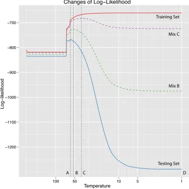
4.3 Phase Transitions . . . 46
4.4 Experiments . . . 50
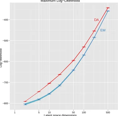
4.4.1 Performance of DA . . . 50
4.4.2 Avoiding overfitting . . . 50
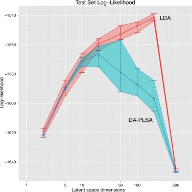
4.4.3 Comparison with LDA . . . 55
4.4.4 Corpus visualization with GTM . . . 57
4.5 Conclusions and Future Work . . . 59
5 summary and future work . . . 60
Appendices . . . 63
a derivatives of the free energy function of da-gtm . . . 63
a.1 First derivatives . . . 64
a.2 Second derivatives . . . 65
b derivatives of the free energy function of da-plsa . . . 66
b.1 First order derivatives . . . 67
b.2 Second order derivatives . . . 67
1
I N T R O D U C T I O N
Finite mixture modeling forms one of the most fundamental foundations in the fields of
statistical pattern recognition, data mining, and machine learning to access the essential
structures of observed random sample data.
It aims at building a probabilistic model in which a random sample is drawn from a
mixture of a finite number of probabilistic distributions called components or sources [24,
36]. The idea is that those components (or sources) can be used to abstract or summarize
the random sample data. However, in general, since no direct information of components
is available initially from a given random sample data, we call such components in a
mixture model as hidden or latent components and the main task in building a finite
mixture model is to uncover such hidden (or latent) components.
Since seeking hidden components or sources to fit observed sample data the best, a
finite mixture model is also called as alatent class modelor atopic model(especially in text
mining area). The process of learning can fall under the category ofunsupervised learning
in that finding latent components is solely based on observed sample data with no use of
any external information. Also, due to its random sample generating capability, a finite
mixture model is known as agenerative model which can randomly generate observable
data.
The finite mixture model provides a flexible and convenient way to explain a wide
variety of random phenomena of observed sample data as a generative process of mixing
finite user-defined random sources [13,24].
introduction 2
Due to its usefulness to provide a flexible and powerful tool of modeling complex
observed data, the finite mixture model has been continued to receive increasing attention
over years, from both a practical and a theoretical point of view [13, 24] and applied
in broad range of areas involving statistical modeling, such as clustering [18, 24], text
mining [5,15], image processing [35], speech recognition [27], to name a few.
One of the main challenges in the finite mixture model is to search an optimal model
parameter set to fit observed sample data, calledmixture model fitting, from a large
param-eter space. In general, the mixture model fitting is known as a NP-hard problem [1]. The
standard method used to fit a finite mixture model is the Expectation-Maximization (EM)
algorithm [12, 13, 24]. However, the EM algorithm for finite mixture model has one
se-rious drawback; it can find only local optimum solutions, not global solutions, and thus
the quality of the answer can be largely affected by initial conditions. We have observed
that a novel global optimization heuristic, called Deterministic Annealing (DA), can
out-perform the traditionalEM algorithm for searching optimal parameters in certain types
of mixture model fitting problems.
The DA algorithm, pioneered by K. Rose and G. Fox [28–31], has been proven its
suc-cess in avoiding local optimum problem and widely used in solving many data mining
algorithms [17, 23,32,37]. Although many researches have been performed on both
the-oretic perspectives [28,37] and clustering applications [17,23, 32,38], the use of theDA,
however, has not been widely reported in many real data mining applications, despite
of its superior quality and overfitting avoidance with a systematic approach. This is the
main topic we study in this work: applying theDA algorithm to solve the finite mixture
model problem and developing new algorithms.
More specifically, in this thesis, we focus two well-known data mining algorithms which
introduction 3
dimension reduction and data visualization, and ii) Probabilistic Latent Semantic
Anal-ysis (PLSA) for text mining. Those two algorithms have been widely used in the fields
of data visualization and text mining, but still suffer from the local optimum problem
due to the use of theEM algorithm in their original developments. Although a DA-like
approach has been discussed in [15], the proposed solution is different from the point
of view of the traditional DA algorithm proposed by K. Rose and G. Fox [28–31]. We
extend thoseEM-based algorithms by using theDA algorithm to improve their qualities
in parameter estimation and overfitting avoidance.
Overfitting is often referred in a supervised learning setting to describe a problem
that a model looses its generality and thus shows large performance differences between
a training set and a validation set. In this thesis, we use overfitting in unsupervised
learning, where we do not have a managed testing set, in order to refer a model with
poor predictive performance for unseen data.
Our contributions in this thesis are summarized as follows:
i) Propose a generalized approach to solve the finite mixture model problem by using a
novel optimization algorithm, calledDA, to guard against the local optimum problem
and help to achieve global optimum solutions.
ii) Develop aDA-based algorithm forGTM, namedDA-GTM.
iii) Present the first and second order differential equations of the new objective function
of DA-GTMfor completing algorithm in deciding starting parameters.
iv) Propose a new fast and stable convergence scheme forDA-GTM.
v) Develop aDA-based algorithm forPLSA, namedDA-PLSA.
vi) Provide the first and second order differential equations of the new objective function
1.1 thesis organization 4
vii) Present experimental results of ourDA-GTMandDA-PLSA, compared with the
tra-ditionalEM-based algorithms.
1.1
thesis organization
The rest of this thesis is orgranized as follows:
• In Chapter 2, we give a broad overview of the finite mixture model and itsEM
al-gorithm as the standard model fitting and parameter estimation method. Especially
we define two finite mixture models we focus in this thesis. We also review theDA
algorithm for the optimal finite mixture model fitting.
• In Chapter 3, we present a DA algorithm for GTM, namedDA-GTM, and
demon-strate the performance results compared with the originalGTMwhich uses an EM
method.
• In Chapter4, we demonstrate how thePLSAproblem can be solved by taking aDA
approach and present a new algorithm, namedDA-PLSA, which is stemmed from
the originalPLSAwhich utilizes anEMoptimization.
1.2 bibliographic notes 5
1.2
bibliographic notes
The work presented in this thesis is solely the outcome of my own research and includes
none of any work in collaboration. Most of theGTMrelated work in this thesis have been
presented and published as conference papers [8–10] and a journal paper [7].
1.3
notation and conventions
In this thesis, we use a normal typeface to indicate scalar values, e.g., σ and β, while using bold typeface for vectors and matrices. To distinguish vectors and matrices, we use
a lower case symbol for vectors, e.g., x, y, and an upper case symbol for matrices, e.g.,
X, Y. We also use an upper case letter for constants without a bold typeface, e.g., N, D. However, exceptions to this convention do appear.
We organize data by using vectors and matrices. We let x1,. . .,xN denote an ob-served or random sample data of size N, where xi is a D-dimensional random row vector (1 6 i 6 N). We organize N-turple sample data into a N×D matrix denoted byX= (xTr1 ,. . .,xTrN)Tr such that rowiof Xcontainsi-th sample dataxn whereTr
repre-sents a transpose. To access each element in a matrix, we use subscripts such that xij is an(i,j) element ofX. Similarly, we lety1,. . ., yK denote component data or latent data of sizeK, whereykis a D-dimensional vector(16k6K). We also organize such K-tuple data set into K×D matrix denoted by Y = (yTr1 ,. . .,yTrK)Tr so that k-th latent vector yk
1.3 notation and conventions 6
We use vectors for an array of scalar values. For example, we let π = (π1,. . .,πK)
denote mixing proportions or weights where each scalar quantity πk(1 6 k 6 K) holds
06πk61and in total
PK
k=1πk =1.
We let|·| andk · kdenote L1-norm andL2-norm, respectively, to represent size of
vec-tors or distances between two vecvec-tors. For example,
|x| = D
X
i=1
|xi| (1.1)
kx−yk =
v u u t
D
X
i=1
2
F I N I T E M I X T U R E M O D E L S A N D D E T E R M I N
-I S T -I C A N N E A L -I N G
In this chapter, we introduce finite mixture models and the Deterministic Annealing (DA)
algorithm.
2.1
finite mixture models
In the finite mixture model, we model the probability distribution of observed sample
data as a mixture distribution of finite number of components in a way in which each
sample is independently drawn from a mixture distribution oflatentorhiddencomponents
of size K with mixing weights. In machine learning, this modeling process falls under the category of unsupervised learning as we aim at finding a model and its parameters
solely from the given sample data without using any external information. In general, we
can assume any form of distributions as a latent component but in practice we use one of
well-defined conventional continuous or discrete distributions, such as Gaussian, Poisson,
multinomial, and so on.
Formally, in the finite mixture model, we model the probability distribution of the
i-th (multivariate) sample data xi as a mixture distribution of K components and
2.1 finite mixture models 8
fine the probability of xi by a conditional probability with a mixing weight vector π =
(π1,. . ., πK)and component-specific parametersΩ={ω1,. . ., ωK}as follows:
P(xi|Ω,π) = K
X
k=1
πkP(xi|ωk) (2.1)
where the parameter set Ωrepresents a general component-specific parameter set; it can
be parameters for latent cluster centers or distribution parameters for components, and
π = {π1,. . .,πK} denotes mixing weights constrained by Pkπk = 1 for all k and each element is bounded by06πk 61.
In general, the mixing weights π1,. . ., πK are system-wide parameters in that all sam-ple data will share the same mixing weights. This model, often called as a mixture of
unigrams [5], is the traditional finite model widely used in the most algorithms,
includ-ing density estimation and clusterinclud-ing, where K components are closely related to the centers of clusters [18]. This is also the model used inGTM[4,10].
Relaxing the condition constrained on the mixing weights, we can further extend the
previous model to build a more flexible model, in a way in which each sample has its own
mixing weights rather than system-wide shared weights used in the previous definition.
This relaxed version of the finite mixture model can be defined by
P(xi|Ω,Ψ) = K
X
k=1
ψikP(xi|ωk) (2.2)
where Ωrepresents a general parameter set as defined above and a new mixing weight
Ψ = {ψ1,. . ., ψN} represents a set of N weight vectors of size K, so that each weight vector ψi represents K mixing weights ψi = (ψi1,. . .,ψiK) corresponding to the i-th sample dataxi and is constrained by
PK
k=1ψik = 1and06ψik61. This is the model
2.1 finite mixture models 9
In this thesis, we focus those two mixture models defined in Eq. (2.1) and Eq. (2.2).
Here-after we call those two finite mixture models as Finite Mixture Model Type-1(FMM-1) and
Finite Mixture Model Type-2(FMM-2) respectively.
2.1.1 Expectation Maximization Algorithm
In analyzing random sample data with finite mixture models, we seek a set of mixture
model parameters so that a model can optimally fit a given sample data set. In statistics,
this process is called model fitting or parameter estimation. One of the most well known
estimators to measure the goodness of fitting or assess the quality of parameters is called
a Maximum Likelihood Estimation (MLE). In the MLE framework, we search a set of
parameters which maximizes likelihood, or equivalently log of likelihood known as
log-likelihood, of a given sample data set.
By using MLE in the finite mixture models defined above, our goal can be stated as
follows; Given that the sample data is independent and identically distributed (i.i.d), the
likelihood of the sample data is
P(X|Ω) = N
Y
i=1
P(xi|Ω) (2.3)
and we seek parameters which maximize the following log-likelihoodL, defined by,
L = logP(X|Ω) (2.4)
= N
X
i=1
2.1 finite mixture models 10
However, finding optimal parameters, i.e., model fitting, by using MLE in finite
mix-ture models is in general intractable except the most trivial cases. Traditionally in finite
mixture models, an iterative optimization method, called EM algorithm developed by
Dempster et al. [12], has been widely used for model fitting.
TheEMalgorithm searches for a solution by iteratively refining local solutions by taking
two consecutive steps per iteration: Expectation step (E-step) and Maximization step
(M-step). The high-level description of the EM steps for the finite mixture models can be
summarized as follows.
• E-step : we evaluate an expectation denoted by rki which is the conditional asso-ciation probability of the k-th component related to the i-th sample data, defined by
rki = P(k|i) (2.6)
= PP(xi|ωk)
k0P(xi|ωk0) (
2.7)
where
K
X
k=1
rki=1 (2.8)
The valuerkiis called in many different ways; responsibility, membership
probabil-ity, and association probability. Basically, it represents how likely samplexican be
2.1 finite mixture models 11
• M-step : using the values computed in E-step, we find parameters which will locally
maximize the log-likelihoodL∗, defined by,
L∗ =
argmax Ω
L (2.9)
= argmax Ω
N
X
i=1
logP(xi|Ω) (2.10)
To determine such parameters, we use the first derivative test; i.e., we compute the
first-order derivatives of Lwith respect to each parameter and test if they become
zero, such that∂L/∂ωk =0. This requires exact knowledge of probability
distribu-tions of components. Thus, details of M-step may vary from different models. The
M-step of our focus algorithms, GTM and PLSA, will be discussed in Section 3.1
and Section4.1respectively.
Although the EMalgorithm has been widely used in many optimization problems
in-cluding the finite mixture models we are discussing, it has been shown a severe limitation,
known as the local optima problem [37], in which theEMmethod can be easily trapped
in local optima, failing to find a global optimum, and so the outputs are very sensitive to
initial conditions. The problem can be worse if we need accurate solutions for, such as,
density estimation or visualization in scientific data analysis. This may also cause poor
quality of query results in text mining.
To overcome such problem occurred in the finite mixture model problems with EM,
including our main focus algorithms GTM [3, 4] and PLSA [15, 16], we apply a novel
optimization method, called DA [28], to avoid local optimum and seek robust solutions
2.2 deterministic annealing 12
2.2
deterministic annealing
TheDAalgorithm [28–31] has been successfully applied to solve many optimization
prob-lems in various machine learning algorithms and applied in many probprob-lems, such as
clustering [17, 28, 38], visualization [23], protein alignment [6], and so on. The core
ca-pability of the DA algorithm is to avoid local optimum and pursue a global optimum
solution in a deterministic way [28], which contrasts to stochastic methods used in the
simulated annealing [22], by controlling the level of randomness or smoothness. TheDA
algorithm, adapted from a physical process known as annealing, finds a solution in a
way in which an optimal solution is gradually revealed as lowering a numerictemperature
which controls randomness or smoothness.
At each level of temperature, theDA algorithm chooses an optimal state by following
the principle of maximum entropy [19–21], developed by E. T. Jaynes, a rational approach
to choose the most unbiased and non-committal answer for a given condition. In short,
the principle of maximum entropy, which is a heuristic approach to be used to choose
an answer with constrained information, states that if we choose an answer with the
largest entropy when other information is unknown, we will have the most unbiased and
non-committal answer.
To find a solution with the largest entropy, theDAalgorithm introduces a new objective
functionF, calledfree energy, an analogy to the Helmholtz free energy in statistical physics,
defined by
F = hDi−TS (2.11)
wherehDirepresents an expected cost,Tis a Lagrange multiplier, also known as anumeric
2.2 deterministic annealing 13
It is known that minimization of the free energy F is achieved when the association
probabilities defined in Eq. (2.6) forms a Gibbs distribution, such as
P(k|i) = exp(−d(i,k)/T) Zi
(2.12)
where d(k,i) represents an association cost between ωk and xi, also called distortion, andZiis a normalization function, also known as partition function in statistical physics.
With Eq. (2.12), we can restate the free energy defined by Eq. (2.11) as
F = −T N
X
i=1
logZi (2.13)
where the partition functionZiis defined by
Zi = K
X
k=1
exp
−d(i,k) T
(2.14)
In the DA algorithm, we choose at each level of temperatures an answer which
mini-mizes the free energy [28]. A standard method of parameter estimation, also known as
model fitting, in finite mixture models is theEM algorithm, which suffers from the local
optimum problem characterized by high-variance answers with different random starts.
To overcome such problem, we use theDAalgorithm which is robust against the random
initialization problem and shows a proven ability to avoid local optimum for finding
2.2 deterministic annealing 14
With the DA algorithm, the traditional objective function based on MLE in the finite
mixture models will be replaced to use the following new objective function based on the
free energy estimation:
F∗=
argmin Ω
F (2.15)
In this thesis, we focus on developing new DAobjective functions forGTM andPLSA
based on the finite mixture models,FMM-1andFMM-2, defined as Eq. (2.1) and Eq. (2.2)
respectively. By using Eq. (2.13), we propose a general free energy function as follows:
FFMM= −T N
X
i=1
log
K
X
k=1
c(i,k)P(xi|ωk)
1/T
(2.16)
wherec(i,k)represents a weight coefficient related with a conditional probability of data
xigiven componentωk,P(xi|ωk).
Details will be discussed in Section3.2and Section4.2respectively.
2.2.1 Phase Transition
As one of the characteristic behaviors of theDAalgorithm, the free energy estimation
un-dergoes an irregular sequence of rapid changes of state, calledphase transitions, when we
are lowering the numeric temperature [28–30]. As a result, at some ranges of temperatures
we cannot obtain all distinctive solutions but, instead, we only obtain a limited number
of effective solutions [28,39]. For an example, in theDA clustering algorithm proposed
by K. Rose and G. Fox [28,30], we can see only one effective cluster at a high temperature
and observe unique clusters gradually pop out subsequently as the temperature is getting
2.2 deterministic annealing 15
Thus, in DA, solutions will be revealed by degrees as the annealing process proceeds,
starting with a high temperature and ending in a low temperature. In other words, as we
do annealing (i.e., lowering temperatures) during theDAprocess, we will observe a series
of specific temperatures, calledcritical temperatures, at which the problem space radically
changes and solutions burst out in a manner in which a tree grows.
A question is how we can find or predict such phase transitions. InDA, we can describe
phase transitions as a moment of losing stability of the objective function, the free energy
F, and turning to be unstable. Mathematically, that moment corresponds to the point
in which the Hessian matrix, the second-order partial derivatives, of the object function
loses its positive definiteness.
In our finite mixture framework, the Hessian matrix, the second-order partial
deriva-tives of the free energyFwith respect to component variablesω1,. . ., ωK, can be defined
as a block matrix:
H =
H11 · · · H1K
..
. ...
HK1 · · · HKK
, (2.17)
where an elementHkk0 is
Hkk0 =
∂2F
∂ωTrk∂ωk0 (
2.18)
for16k,k06K.
At a critical temperature (a moment of a phase transition), the Hessian Hwill be
un-stable and lose its positive definiteness. This temperature is called a critical temperature.
Thus, we can define critical temperatures as the point to make the determinant of Hessian
2.2 deterministic annealing 16
Iteration
Te
mp
1 2 3 4 5
200 400 600 800 1000
(a)exponential
Iteration
Te
mp
2 3 4 5
200 400 600 800 1000
(b)linear
Iteration
Te
mp
1 2 3 4 5
200 400 600 800 1000 1200
(c)adaptive
Figure 1:Various cooling schedule schemes. While exponential (a) and linear (b) is fixed and pre-defined, our new cooling scheme (c) is adaptive that the next temperature is determined in the on-line manner.
We will cover details of derivation and usages for GTM and PLSA in Section3.3 and
Section4.3respectively.
2.2.2 Adaptive cooling schedule
The DA algorithm has been applied in many areas and proved its success in avoiding
local optimum and pursuing global solutions. However, to the best of our knowledge, no
literature has been found about the cooling schedule of the DA algorithm. Commonly
used cooling schedule is exponential (Figure 1a), such asT = αT , or linear (Figure 1b),
such asT =T−δ for invariant coefficientsαandδ. Those scheduling schemes are fixed in that cooling temperatures are pre-defined and the coefficientαorδwill not be changed during the annealing process, regardless of the complexity of a given problem.
However, as we discussed previously, the DA algorithm undergoes the phase
transi-tions in which the problem space (or free energy) can change dramatically. To avoid such
drastic changes and make the transitions smoother, one may try to use very smallαor δ
2.2 deterministic annealing 17
To overcome such problem, we propose an adaptive cooling schedule in which cooling
temperatures are determined dynamically during the annealing process. More
specifi-cally, at every iteration in theDA algorithm, we predict the next phase transition
temper-ature and move to that tempertemper-ature as quickly as possible. Figure1c shows an example
of an adaptive cooling schedule, compared with fixed cooling schedules, Figure 1a and
Figure1b.
Another advantage we can expect in using our adaptive cooling schedule scheme is that
users have no need to set anymore coefficients regarding cooling schedule. The adaptive
cooling process will automatically suggest next temperatures, based on a given problem
complexity. The adaptive cooling schedule forGTMwill be discussed in Section3.3.
2.2.3 Overfitting Avoidance
In statistical machine learning, overfitting (or overtraining) is a phenomena that a trained
model works too well on the training example but shows poor predictive performance
on unseen data [2, 25]. Especially in a supervised learning setting, an overfitting
prob-lem can be observed when training errors are getting smaller while validation errors
are increasing. Such overfitting problem, in general, contributes to the poor predictive
power of a trained model and causes a serious issue in many statistical machine
learn-ing, data minlearn-ing, and information retrieval where predictive power for unseen data is
a valuable property. A few general solutions suggested in the areas are regularization,
cross-validation, early stopping, and so on.
In this thesis, we use DA in the finite mixture model framework to guard against the
overfitting problem in an unsupervised learning setting where we do not have a managed
2.2 deterministic annealing 18
Besides avoiding local optima problem discussed earlier,DAcan also provide a
capabil-ity for overfitting avoidance finding a generalized solution. In fact,DAnatively supports
generalized solutions. Note that DA starts to find a model in a smoothed probability
surface in a high numeric temperature and gradually tracking an optimum solution in
a bumpy and complex probability surface on lowering the numeric temperature [26]. In
other words, DA has naturally an ability to control smoothness of a solution. We can
exploit this feature ofDAto obtain a less- or non-overfitted model.
Overfitting avoidance ofDAhas been investigated in various places [16,33,34]. In this
thesis, we take a similar approach to exploit DA’s overfitting avoidance for improving
predicting power for PLSA, a text mining algorithm. Details will be discussed in
3
G E N E R A T I V E T O P O G R A P H I C M A P P I N G W I T H
D E T E R M I N I S T I C A N N E A L I N G
In this chapter, we introduce the Generative Topographic Mapping (GTM) algorithm and
describe how the GTM problem can be solved in the finite mixture model framework.
Especially, we show the GTM algorithm is based on the Finite Mixture Model Type-1
(FMM-1), defined in Eq. (2.1). Then, we propose a new DA algorithm for GTM, named
Generative Topographic Mapping with Deterministic Annealing (DA-GTM). In the next,
we start with brief overviews of the GTM problem and discuss how we use the DA
algorithm for parameter estimation inGTMand predicting phase transition inDA-GTM,
followed by experimental results.
3.1
generative topographic mapping
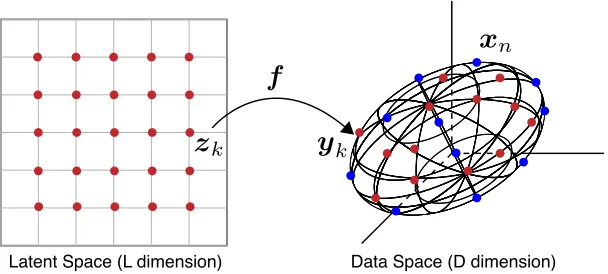
TheGTM[3,4] algorithm is a visualization algorithm designed to find a non-linear
mani-fold embedding in a low dimension space (say,L-dimension) for a given high dimensional data set (sayD-dimensional) by using Klatent components. More specifically, the GTM
algorithm seeks K latent variables, denoted by z1,. . .,zK, in L-dimension space, also
called latent space, such that zk ∈ RL(k = 1, ...,K), which can optimally represent the
3.1 generative topographic mapping 20
Data Space (D dimension) Latent Space (L dimension)
z
ky
k [image:31.612.180.484.124.261.2]x
nf
Figure 2:Non-linear embedding by GTM
given Ndata points, denoted by x1,. . .,xN, in the D-dimension space, also called data space, which usuallyLD(See Figure2).
For this end, the GTM algorithm finds a low dimensional embedding by using the
following two steps: First, mapping theKlatent variables,z1,. . .,zK, in the latent space
to the data space with respect to a non-linear mapping f : RL 7→ RD. Let us denote
the mapped points in the data space asy1,. . .,yK. Secondly, fitting the mapped points
y1,. . .,yK, considered asKcomponents, to theNsample data pointsx1,. . .,xNby using
FMM-1defined in Eq. (2.1).
Note that the GTMalgorithm uses explicitly the Gaussian probability as a component
distribution, specifically, defined by a Gaussian centered onyk with covarianceΣk.
With-out losing generality, we assume the Gaussian as an isotropic Gaussian with scalar
vari-anceσ2, such that the conditional probability density P(xi|yk,σ2) is defined by the
fol-lowing Gaussian distributionN:
P(xi|yk,σ2) = N(xi|yk,σ2) (3.1)
=
1 2πσ2
D/2
exp
− 1
2σ2 kxi−ykk 2
3.1 generative topographic mapping 21
In summary, theGTMalgorithm is theFMM-1in which a sample data is modeled by
P(xi|Y,σ2) = K
X
k=1 1
K N(xi|yk,σ 2)
. (3.3)
In the GTMalgorithm, we uses an uniform mixing weight, such that πk = 1/K for all
k (1 6 k 6 K), as the Gaussian can control its variance σ2 for varying mixing weights. Also, the component variables y1,. . .,yK, serving as centers of Gaussian or means, are
mapped by a non-linear function from L-dimension to D-dimension. The choice of the non-linear mapping f : RL 7→ RD can be made from any parametric, non-linear model.
In the originalGTMalgorithm [3,4], a generalized linear regression model has been used,
in which the map is a linear combination of a set of fixedMbasis functions, such that,
yk =φTrkW, (3.4)
where a column vectorφk = (φk1, ...,φkM) is a mapping ofzk by theMbasis function φm : RL 7→ R for m = 1, ...,M, such that φkm = φm(zk) and W is a M×D matrix
containing weight parameters. With a matrix notation, we can simplify the above equation
by
Y =ΦW (3.5)
3.2 deterministic annealing for generative topographic mapping 22
With this model setting, theGTMalgorithm corresponds to a Gaussian mixture model
problem of FMM-1 and seeks an optimal set of parameters, y
1,. . ., yK and σ2, which
maximizes the following log-likelihood ofGTM,LGT M, defined by
LGT M(Y,σ2) =
N
X
i=1
log
1 K
K
X
k=1
N(xi|yk,σ2)
(3.6)
3.2
deterministic annealing for generative topographic
mapping
TheGTMalgorithm uses anEMmethod which starts with a random initial matrixWand
iteratively refines a solution to maximize Eq. (3.6), which can be easily trapped in local
optima. Thus, an output (which is a mapping) produced by the originalGTMalgorithm
can vary depending on initial parameters, which is known as the random initial value
problem. Instead of using the EM, we have applied a DA approach to find a global
optimum solution. With the use of the DA algorithm, we can have more robust GTM
maps without suffering the random initial value problem.
To apply the DA algorithm, as discussed in Section 2.2, we need a new free energy
function forGTM, namedFGT M, which we will minimize through iterations. By using the
3.2 deterministic annealing for generative topographic mapping 23
function for theGTMalgorithm as follows; First, we let define the association costd(n,k)
using a Gaussian distribution by
d(i,k) = −log P(xi,yk) (3.7)
= −log {P(yk)P(xi|yk)} (3.8)
= −log
1
K N(xi|yk,σ 2)
(3.9)
By using Eq. (2.12), then, we can defineZiby
Zi = K
X
k=1
1 K
β
N(xi|yk,σ2)β (3.10)
Here, for brevity, we use aninverse numeric temperaturedenoted byβ, such thatβ=1/T. Finally, by using Eq. (2.13), we can have the free energy function for GTM, FGT M, as
follows:
FGT M(Y,σ2,β) = −
1 β
N
X
i=1
logZi (3.11)
= −1 β
N
X
i=1
log
1 K
βXK
k=1
N(xi|yk,σ2)β
(3.12)
which is the objective function for the DA-GTMalgorithm to minimize as changing
tem-perature from high (equivalentβnear zero) and to low (equivalentlyβ=1.0).
Notice that the free energy function of DA-GTM, FGT M (3.12), and the MLE (3.6) of
GTMdiffer only the use of the inverse temperature variableβand the sign. Especially, at
β=1.0, we have
3.2 deterministic annealing for generative topographic mapping 24
and thus we can conclude that the originalGTMalgorithm’s target functionLGT Mis just
a special case ofFGT M.
To minimize (3.12), we need to find parameters to make the following two partial
derivatives be zero (Detailed derivations can be found in AppendixA):
∂FGT M
∂yk = 1 σ2
N
X
i=1
ρki(xi−yk) (3.14)
∂FGT M
∂σ2 = −σ 4
N
X
i=1 K
X
k=1 ρki
Dσ2 2 −
1
2kxi−ykk 2
(3.15)
whereρki is a property, known asresponsibility, such that,
ρki =
P(xi|yk,σ2)β
PK
k0=1P(xi|yk0,σ2)β
(3.16)
By using the same matrix notations used in the GTM paper [3, 4], the DA-GTM
algo-rithm can be written as a process to seek an optimal weightW and variance σ2 at each temperatureT.
W = (ΦTrGΦ)−1ΦTrRX (3.17)
1 σ2 =
1 ND
N
X
i=1 K
X
k=1
ρkikxi−ykk2 (3.18)
3.3 phase transitions 25
3.3
phase transitions
As we discussed in Section 2.2, DA algorithms undergoes phase transitions as lowering
the temperatures. At some temperature, we can not obtain all distinct solutions but,
instead, we can only obtain a number of effective solutions. All solutions will gradually
pop out while the annealing process proceeds as with lowering the temperature.
In the DA-GTM algorithm, we can observe the same behavior. As an example, at
a very high temperature, the DA-GTM algorithm gives only one effective latent point
that all yk’s are collapsed to, corresponding to the center of data, denoted by ¯x, such
that ¯x = PNi=1xi/N. At a certain temperature as we lowering temperature gradually,
components,y1,. . ., yK, which were settled(or stable) in their positions, start to explode
(or move). We call this temperature as the first critical temperature, denoted by T(1)c or,
equivalently, β(1)c = 1/Tc(1), where the superscript indicates a sequence. As we further
lowering the temperature, we can observe a series of subsequent phase transitions and
thus multiple critical temperatures, such as T(2)c ,Tc(3),. . .,T(K)c . Especially obtaining the
first phase transitionT(1)c is an important task since we should start our annealing process
with an initial temperature higher thanT(1)c .
In theDAalgorithm, we define a phase transition as a moment of losing stability of the
DA’s objective function, the free energy F, and turning to be unstable. Mathematically,
that moment corresponds to the status in which the Hessian of the object function loses
3.3 phase transitions 26
For our DA-GTM algorithm, we can write the following Hessian matrix as a block
matrix:
H =
H11 · · · H1K
..
. ...
HK1 · · · HKK
, (3.19)
where a sub matrixHijis a second derivative of the free energyFGT Mas shown in Eq. (2.11).
More specifically,Hijcan be written as follows:
Hkk =
∂2FGT M
∂yTrk∂yk (
3.20)
= − 1 σ4T
N
X
i=1
ρki(1−ρki)(xi−yk)Tr(xi−yk) −Tσ2ρkiID , or (3.21)
Hkk0 =
∂2FGT M
∂yTr
k∂yk0
(3.22)
= 1 σ4T
N
X
i=1
−ρkiρk0n(xi−yk)Tr(xi−yk0) (k6=k0), (3.23)
wherek,k0 =1,. . .,K, andIDis an identity matrix of sizeD. Note thatHkkandHkk0 are D×Dmatrices and thus,H∈RKD×KD.
As discussed in Section2.2.1, we can compute the critical points which satisfy det(H) = 0. However, the size of the hessian matrixHcan be too big to compute in practice. Instead, we compute critical points by dividing the problem into smaller pieces. The sketch of the
algorithm is as follows:
1. For each componenty
3.3 phase transitions 27
2. Compute a local Hessian fory
k (let denoteHk) defined by
Hk =
Hkk Hkk0
Hkk0 Hkk
(3.24)
whereHkk andHkk0 are defined by Eq. (3.20) and Eq. (3.22) respectively but we let ρki=ρki/2as we divide responsibilities too. Then, find a candidate of next critical temperatureTc,k by letting det(Hk) =0.
3. Choose the most largest yet lower than the current T among {Tc,k} for all k =
1,. . .,K.
To compute det(Hk) =0, let define the following:
Ux|yk =
N
X
i=1
ρki(xi−yk)Tr(xi−yk) (3.25)
Vx|yk =
N
X
i=1
(ρki)2(xi−yk)Tr(xi−yk) (3.26)
Then, we can rewrite Eq. (3.20) and Eq. (3.22) by
Hkk = − 1
Tσ4 2Ux|yk−Vx|yk−2Tσ
2γkID
(3.27)
Hkk0 = − 1
Tσ4 −Vx|yk
(3.28)
We can also rewrite Eq. (4.19) by
Hk = − 1 Tσ2
2Ux|yk−Vx|yk −Vx|yk
−Vx|yk 2Ux|yk−Vx|yk
−2Tγkσ
2I 2D
3.3 phase transitions 28
Thus, by letting det(H) =0, we get the following eigen equation:
eig
2Ux|yk−Vx|yk −Vx|yk
−Vx|yk 2Ux|yk−Vx|yk
= 2Tγkσ
2
(3.30)
where eig(A)denotes eigenvalues ofA.
We can further simplify the above equation by using the Kronecker product⊗:
eig
2 0 0 2
⊗Ux|yk−
1 1 1 1
⊗Vx|yk
= 2Tγkσ
2
(3.31)
Finally,Tc,k can be computed by
Tc,k = 1 2γkσ2
λmax,k (3.32)
where λmax,k is the largest, but lower than a current temperature T, eigenvalue of the lefthand side of Eq. (3.31).
The first critical temperature Tc(1) is a special case of Eq. (3.32). With the Hessian
matrix defined above, we can compute the first phase transition point occurred at T(1)c .
Assuming that the system has not yet undergone the first phase transition and the current
temperature is high enough, then we will have all yk’s overlapped in the center of the
data point, denoted by y0 = x¯ = PNi=1xi/N, and equal responsibilities, such as ρki = ρk0n=1/2for allkandn.
Then, the second derivatives can be rewritten by
Hkk = − N
4Tσ4 Sx|y0−2T σ
2I D
(3.33)
Hkk0 = − N
4Tσ4 −Sx|y0
3.3 phase transitions 29
Algorithm1GTM with Deterministic Annealing
DA-GTM
1: SetT > Tcby using Eq. (3.37)
2: Choose randomly M basis function
φm(m=1, ...,M)
3: Compute Φ whose element φkm =
φm(zk)
4: Initialize randomlyW
5: Computeσ2by Eq. (3.18) 6: whileT >1do
7: UpdateWby Eq. (3.17)
8: Updateσ2 by Eq. (3.18) 9: T ←NextCriticalTemp
10: end while
11: return Φ,W,σ2
Algorithm2Find the next critical temperature NextCriticalTemp
1: fork=1toKdo
2: Λk←{∅}
3: foreachλ∈eig
Ux|yk−Vx|yk
do
4: ifλ < T γkσ2 then
5: Λk←Λk∪λ 6: end if
7: end for
8: λmax,k←max(Λk) 9: Tc,k←λmax,k/γkσ2 10: end for
11: return Tc←max({Tc,k})
whereSx|y0 represents a covariance matrix of centered data set such that,
Sx|y0 =
1 N
N
X
i=1
(xi−y0)Tr(xi−y0) (3.35)
and the Hessian matrix also can be rewritten by
eig
1 −1 −1 1
⊗NSx|y0
= 2Tγkσ
2 (3.36)
Thus, the first critical temperature is
Tc= 1
σ2λmax (3.37)
whereλmax is the largest eigenvalue ofSx|y0.
With Eq. (3.32) and Eq. (3.37), we can process DA-GTM with an adaptive cooling
scheme discussed in Section 2.2.2. The overall pseudo code is shown in Algorithm 1
3.4 experiments 30
Maximum Log−Likelihood = 1532.555
Dim1 Dim2 −1.0 −0.5 0.0 0.5 1.0 ● ● ● ● ● ● ● ● ● ● ● ● ● ● ● ● ● ● ● ● ● ● ● ● ● ● ● ● ● ● ● ● ● ●● ● ● ● ● ● ● ● ● ● ● ● ● ● ●● ● ●● ● ● ● ● ● ● ● ● ● ● ● ● ● ●● ● ● ● ● ● ● ● ● ●● ● ● ● ● ● ● ● ● ● ● ● ● ● ● ● ● ● ● ● ● ● ● ● ● ● ● ● ● ● ● ● ●● ● ● ● ● ● ● ● ● ● ● ● ● ● ● ● ● ● ● ● ● ● ● ● ● ● ● ● ● ● ● ● ● ● ● ● ● ● ● ● ● ●● ● ● ● ● ● ● ● ● ● ● ● ● ● ● ● ● ● ● ● ● ● ● ● ● ● ● ● ● ● ● ● ● ● ● ● ● ● ● ● ● ● ● ● ● ● ● ● ● ● ● ● ● ● ● ● ● ●● ● ● ● ● ● ● ● ● ● ● ● ● ● ● ● ● ● ● ● ● ● ● ● ● ● ● ● ● ● ● ● ● ● ● ● ● ● ● ● ● ● ● ● ● ● ● ● ● ● ● ● ● ● ● ● ● ● ● ● ● ● ● ● ● ● ● ● ● ● ● ● ● ● ● ● ● ● ● ● ● ● ● ● ● ● ● ● ● ● ● ● ● ● ● ● ● ● ● ● ● ● ● ● ● ● ● ● ● ● ● ● ● ● ● ● ● ● ● ● ● ● ● ● ● ● ● ● ● ● ● ● ● ● ● ● ● ● ● ● ● ● ● ● ● ● ● ● ● ● ● ● ● ● ● ● ● ● ● ● ● ● ● ● ● ● ● ● ● ● ● ● ● ● ● ● ● ● ● ● ● ● ● ● ● ●● ● ● ● ● ● ● ● ● ● ● ● ● ●● ● ● ● ● ● ● ● ● ●● ● ● ● ● ● ● ● ● ● ● ● ● ● ● ● ● ● ● ● ● ● ● ● ● ● ● ● ● ● ● ● ●● ● ● ● ● ● ● ● ● ● ● ● ● ● ● ● ● ● ● ● ● ● ● ● ● ● ● ● ● ● ● ● ● ● ● ● ● ● ● ● ● ● ● ● ● ● ● ● ● ● ● ● ● ● ● ● ● ● ● ● ● ● ● ● ● ● ● ● ● ● ● ● ● ● ● ● ● ● ● ● ● ● ● ● ● ● ● ● ● ● ● ● ● ● ● ● ● ● ● ●● ● ● ● ● ● ● ● ● ● ● ● ● ● ● ● ● ● ● ● ● ● ● ● ● ● ● ● ● ● ● ● ● ● ● ● ● ● ● ● ● ● ● ● ● ● ● ● ● ● ● ● ● ● ● ● ● ● ● ● ● ● ● ● ● ● ●● ● ● ● ● ● ● ● ● ● ● ● ● ● ● ● ● ● ● ● ● ● ● ● ● ● ● ● ● ● ● ● ● ● ● ● ● ● ● ● ● ● ● ● ● ● ● ● ● ● ● ● ● ● ● ● ● ● ● ● ● ● ● ● ● ●
−1.0 −0.5 0.0 0.5 1.0
(a)EM-GTM
Maximum Log−Likelihood = 1636.235
Dim1 Dim2 −1.0 −0.5 0.0 0.5 1.0 ● ● ● ● ● ● ● ● ● ● ● ● ● ● ● ● ● ● ● ● ● ● ● ● ● ● ● ● ● ● ● ● ● ● ● ● ● ● ● ● ● ● ● ● ● ● ● ● ● ● ● ● ●● ●● ● ● ● ● ● ● ● ● ● ●●● ● ● ● ● ● ● ● ● ● ● ● ● ● ● ●● ● ● ● ● ● ● ● ● ● ● ● ● ● ● ● ● ● ● ● ● ● ● ● ● ● ● ● ● ● ● ● ● ● ● ● ● ● ● ● ● ● ● ● ● ● ● ● ● ● ● ● ● ● ● ● ● ● ● ● ● ● ● ● ● ● ● ● ● ● ● ● ● ● ● ● ● ● ● ● ● ● ● ● ● ● ● ● ● ● ● ● ● ● ● ● ● ● ● ● ● ●● ● ● ● ● ● ● ● ● ●● ● ● ●● ● ● ● ● ● ● ● ● ● ● ● ● ● ● ● ● ● ● ● ● ● ● ● ● ● ● ● ● ● ● ● ● ● ● ● ● ● ● ● ● ● ● ● ● ● ● ● ● ● ● ● ● ● ● ● ● ● ● ● ● ● ● ● ● ● ● ● ● ● ● ● ● ●● ● ●● ● ● ● ● ● ● ● ● ● ● ● ● ● ● ● ● ● ● ● ● ● ● ● ● ● ● ● ● ● ● ● ● ● ● ● ● ● ● ● ● ● ● ●● ● ● ● ● ● ● ● ● ● ● ● ● ● ● ● ● ● ● ● ● ● ● ● ● ● ● ● ● ● ● ● ● ● ● ● ● ● ● ● ● ● ● ● ● ● ● ● ● ● ● ● ● ● ● ● ● ● ● ● ● ● ● ● ● ● ● ● ● ● ● ● ● ● ● ● ● ● ● ● ● ● ● ● ● ● ● ● ● ● ● ● ● ● ● ● ● ● ● ● ● ● ● ● ● ● ● ● ● ● ● ● ● ● ● ● ● ● ● ● ● ● ● ● ● ● ● ● ● ● ● ● ● ● ● ● ● ● ● ● ● ● ● ● ● ● ● ● ● ● ● ● ● ● ● ● ● ● ● ● ●● ● ● ● ● ● ● ● ● ● ● ● ● ● ● ● ● ● ● ● ● ● ● ● ● ● ● ● ● ● ● ● ● ● ● ● ● ● ● ● ● ● ● ● ● ● ●● ● ● ● ● ● ● ● ● ●● ● ● ●● ● ● ● ● ● ● ●● ● ● ● ● ● ● ● ● ● ● ● ● ● ● ● ● ● ● ● ● ● ● ● ● ● ● ● ● ● ● ● ● ● ● ● ● ● ● ● ● ● ● ● ● ● ● ● ● ● ● ● ● ● ● ● ● ● ● ● ● ● ● ● ●● ● ● ● ● ● ● ● ● ● ● ● ● ● ● ● ● ● ● ● ● ● ● ● ● ● ● ● ● ● ● ● ● ● ● ● ● ● ● ● ● ● ● ● ● ● ● ● ● ● ● ● ● ● ● ● ● ● ● ● ● ● ● ● ● ● ● ● ● ● ●
−1.0 −0.5 0.0 0.5 1.0
(b)DA-GTM with exp. scheme
Maximum Log−Likelihood = 1721.554
Dim1 Dim2 −1.0 −0.5 0.0 0.5 1.0 ● ● ● ● ● ● ● ● ● ● ● ● ● ● ● ● ● ● ● ● ●● ● ● ● ● ● ● ● ● ● ● ● ● ● ● ● ● ● ● ● ● ● ● ● ● ● ● ● ● ● ● ● ● ● ● ● ● ● ● ● ● ● ● ● ● ● ● ● ● ● ●● ● ● ● ●● ● ● ● ● ● ● ● ● ● ● ● ● ● ● ● ● ● ● ● ● ● ● ● ● ● ● ● ● ● ● ● ● ● ● ●● ● ● ● ● ● ● ● ● ● ● ● ● ● ● ● ● ● ● ● ● ● ● ● ● ● ● ● ● ● ● ● ● ● ● ● ● ● ●● ● ● ● ● ● ● ● ●● ● ● ● ● ● ● ● ● ● ● ● ● ● ● ● ● ● ● ● ● ● ● ● ● ● ● ● ● ● ● ● ● ● ● ● ● ● ● ● ● ● ● ● ● ● ● ● ●● ● ● ● ● ● ● ● ● ● ● ● ● ● ● ● ● ● ● ● ● ● ● ● ● ● ● ● ● ● ● ●● ● ● ● ● ●● ● ● ● ● ● ● ● ● ● ● ● ● ● ● ● ● ● ● ● ● ● ● ● ● ● ● ●● ● ● ● ● ● ● ● ● ● ● ● ● ● ● ● ● ● ● ● ● ● ● ● ● ● ● ● ● ● ● ● ● ● ● ● ● ● ● ● ● ● ● ●● ● ● ● ● ● ● ● ● ● ● ● ● ● ● ● ● ● ● ● ● ● ● ● ● ● ● ● ● ● ● ● ● ● ● ● ● ● ● ● ● ● ● ●● ● ● ● ● ● ● ● ● ● ● ● ● ● ● ● ● ● ● ● ● ● ● ● ● ● ● ● ● ● ● ● ● ● ● ● ● ● ● ● ● ● ● ● ● ● ● ● ● ● ● ● ● ● ● ●● ● ● ● ● ● ● ● ● ● ● ● ● ● ● ● ● ● ● ● ● ● ● ● ● ● ● ● ● ● ● ● ● ● ● ● ● ● ● ● ● ● ● ● ● ● ● ● ● ● ● ● ● ● ● ● ● ● ● ● ● ● ● ● ● ● ● ● ● ● ● ● ● ● ●● ● ● ● ● ● ● ● ● ● ● ● ● ● ● ● ● ● ● ● ● ● ● ● ● ● ● ● ● ● ● ● ● ● ● ● ● ● ● ● ● ● ● ● ● ● ● ● ● ● ● ● ● ● ● ● ● ●● ● ● ● ● ● ● ● ● ● ● ● ● ● ● ● ● ● ● ● ● ● ● ● ● ● ● ● ● ● ●● ● ● ● ● ● ●● ● ● ● ● ● ● ● ● ● ● ● ● ● ● ● ● ● ● ● ● ● ● ● ● ● ● ●● ● ● ● ● ● ● ● ● ● ● ● ● ● ● ● ● ● ● ● ● ● ● ● ● ● ● ● ● ● ● ● ● ● ● ● ● ● ● ● ● ● ● ● ● ● ● ● ● ● ● ● ● ● ● ● ● ● ● ● ● ● ● ● ● ● ●
−1.0 −0.5 0.0 0.5 1.0
(c)DA-GTM with adaptive scheme
Labels
A B C
Figure 3:Comparison of (a) EM-GTM, (b) DA-GTM with exponential, and (c) DA-GTM
with adaptive cooling scheme for the oil-flow data which has 3-phase clusters
(A=Homogeneous, B=Annular, and C=Stratified configuration). Plots are drawn by a
median result among 10 random-initialized executions for each scheme. As a result,
DA-GTM with adaptive cooling scheme (c) has produced the largest maximum log-likelihood and thus the plot shows better separation of the clusters, while EM-GTM (a) has output the smallest maximum log-likelihood and the result shows many overlaps.
3.4
experiments
To compare the performances of our DA-GTM algorithm with the original EM-based
GTM (hereafter EM-GTM for short), we have performed a set of experiments by using
two datasets: i) the oil flow data used in the original GTM papers [3, 4], obtained from
the GTM website1
, which has1,000points having12dimensions for3-phase clusters and
ii) a chemical compound data set obtained from PubChem database2
, which is a
NIH-funded repository for over60million chemical compounds and provides various chemical
information including structural fingerprints and biological activities, for the purpose of
chemical information mining and exploration. In this paper we have randomly selected a
subset of1,000elements having166dimensions.
1 GTM homepage,http://www.ncrg.aston.ac.uk/GTM/
3.4 experiments 31
Start Temperature
Log−Lik
elihood (llh)
0.0 0.5 1.0 1.5 2.0
N/A 5 7 9
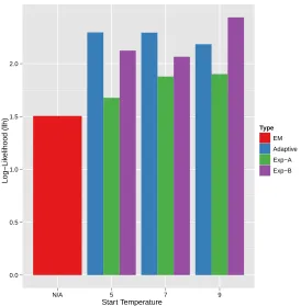
[image:42.612.183.457.114.393.2]Type EM Adaptive Exp−A Exp−B
Figure 4:Comparison of EM-GTM with DA-GTM in various settings. Average of 10 random
initialized runs are measured for EM-GTM, DA-GTM with3cooling schemes (adaptive,
exponential withα=0.95(Exp-A) andα=0.99(Exp-B).
In Figure3, we have compared for the oil-flow data maximum log-likelihood produced
by EM-GTM, DA-GTM with exponential cooling scheme, and DA-GTM with adaptive
cooling scheme and present corresponding GTM plots as outputs, known as
posterior-mean projection plot [3, 4], in the latent space. For each algorithm, we have executed 10
runs with different random setups, chosen a median result, and drawn a GTM plot. As
a result, DA-GTM with adaptive cooling scheme (Figure 3c) has produced the largest
maximum log-likelihood (best performance), while EM-GTM (Figure 3a) produced the
smallest maximum log-likelihood (worst performance). Also, as seen in the figures, a
3.4 experiments 32
Iteration
Log−Li
kelihood
value
−8000 −6000 −4000 −2000 0 2000
2000 4000 6000 8000
Type
Likelihood
Average Log-Likelihood of EM-GTM
(a)Progress of log-likelihood
Iteration
Tempe
rature
1 2 3 4 5 6 7 ●●●●●●●●
● ● ● ● ● ● ● ● ● ● ● ● ● ● ● ● ● ● ●●●●●●●●●
● ● ● ● ●
2000 4000 6000 8000
Type
● Temp
Starting Temperature
1st Critical Temperature
(b)Adaptive changes in cooling schedule
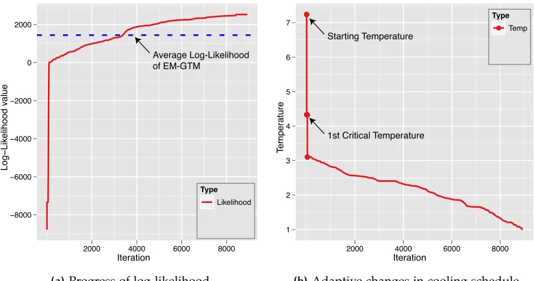
Figure 5:A progress of GTM with adaptive cooling schedule. This example show how DA-GTM with adaptive cooling schedule progresses through iterations
In the next, we have compared the performance ofEM-GTMandDA-GTMwith 3
dif-ferent cooling schemes: i) Adaptive schedule, which we have prosed in this thesis, ii)
Ex-ponential schedule with a cooling coefficientsα=0.95(denoted Exp-A hereafter), and iii) Exponential schedule with a cooling coefficientsα=0.99 (denoted Exp-B hereafter). For eachDA-GTM setting, we have also applied3 different starting temperature 5, 6, and 7,
which are all larger values than the1st critical temperature which is about4.64computed by Eq. (3.37). Figure4 shows the summary of our experiment results in which numbers
are estimated by the average of10executions with different random initialization.
As a result shown in Figure 4, the DA-GTMoutperformsEM-GTM in all cases. Also,
our proposed adaptive cooling scheme mostly outperforms other static cooling schemes.
Figure 5shows an example of execution ofDA-GTMalgorithm with adaptive cooling
[image:43.612.128.518.118.323.2]