Road Traffic Congestion Solution using Discrete Event Simulation

International Journal of Innovative Technology and Exploring Engineering (IJITEE) ISSN: 2278-3075, Volume-8 Issue-5S March, 2019

Abstract: The increasing number of vehicles in developing areas indirectly become one of the causes for road traffic conges-tion (RTC) to occur. RTC can also be caused by a temporary obstruction, a permanent capacity bottleneck in the network itself, stochastic fluctuation in demand within a network, leading to spillback and queue propagation. Inefficient management of traffic light control (TLC) to the existing system in term of cycle time contributes to the RTC in a developing town in Malaysia, Changloon, especially during peak hours that lead to environ-mental pollution and long average waiting time. This situation negatively affects the road users and the people surrounding. A discrete-event simulation (DES) model was developed using ARENA software to represent the real TLC system condition during peak hours. From the simulation model, the TLC which causing the bottleneck was identified. The total of three scenarios were developed with modification on elements such as road struc-ture and cycle time of TLC. All scenarios recorded with im-provement for total average waiting time and average number in queue. The findings of this study can be used as a guideline for authorities to improve road traffic at Changloon town during peak hours.

Keywords: Cycle time; discrete-event simulation; road traffic conges-tion; traffic light control; waiting time

I.

INTRODUCTION

Basically, there are two types of road transportation. The first type is private transportation and the other one is public transportation. In Malaysia, people more favor to use private transportation instead of public transportation. This is due to many factors including poor services’ quality of public transportation [1]. This situation occurs not only in big cities but also in a small town like Changloon. Statistics provided by Road Transport Department, Malaysia [2] prove that the total registered vehicles from 2010 to 2015 is increasing drastically as shown in Figure 1.

Revised Manuscript Received on March 08, 2019

Muhammad Zulqarnain Hakim Abd Jalal, School of Quantitative Sciences, Universiti Utara Malaysia, 06010 UUM Sintok, Kedah, Malaysia

Wan Laailatul Hanim Mat Desa, School of Quantitative Sciences, Universiti Utara Malaysia, 06010 UUM Sintok, Kedah, Malaysia

Mohd Kamal Mohd Nawawi, Institute of Strategic Industrial Decision Modelling (ISIDM), School of Quantitative Sciences, Universiti Utara Malaysia, 06010 UUM Sintok, Kedah, Malaysia. mdkamal@uum.edu.my

Ruzelan Khalid, Institute of Strategic Industrial Decision Modelling (ISIDM), School of Quantitative Sciences, Universiti Utara Malaysia, 06010 UUM Sintok, Kedah, Malaysia

Razamin Ramli, School of Quantitative Sciences, Universiti Utara Ma-laysia, 06010 UUM Sintok, Kedah, Malaysia

Waleed Khalid Abduljabbar, School of Quantitative Sciences, Universiti Utara Malaysia, 06010 UUM Sintok, Kedah, Malaysia

Hence, with raging growth in private vehicle purchase and practice, this will lead to road traffic congestion (RTC).

Fig. 1Total registered vehicles in Malaysia up to year

2015 [2]

RTC can occur at anywhere and it can either be predicta-ble or unpredictapredicta-ble. There is nothing can be done with un-predictable event as it happened outside the expectation while not for predicted event which occurs at the main road, and mostly controlled by traffic light system. Traffic light control (TLC) optimization have received special attention in recent years. From the previous studies, most of RTC closely related to weak traffic control system or more pcisely an inefficient TLC system [3]–[7]. Therefore, re-search in reducing RTC by optimizing TLC system is rele-vant to be studied where the focus of this study is at Changloon main road traffic system in Malaysia.

The main objective for this paper is to control road traffic congestion at Changloon major road. There are four sub-objectives need to be completed, to achieve the main objec-tive. The sub-objectives of this study are; to develop a model to simulate current road traffic at Changloon main road, to identify which TLC causing RTC at Changloon main road, to construct what-if analysis with the aim to re-duce RTC at Changloon main road, and finally to provide alternatives for the improvement of Changloon's main road traffic conditions.

II. LITERATURE REVIEW

RTC is no more an odd problem and continues to become a major global problem. Mobility necessity turns transporta-tion systems as an essential element in lives and the amount of vehicles roaming on the street and road

Road Traffic Congestion Solution using

Discrete-Event Simulation

strikingly increase from year to year [8]. This problem is deteriorating when it comes to a fast developing areas or commercial areas [9]. As the outcomes from this issue, it can cause massive delays, increased fuel wastage and mone-tary losses [10]. According to Downie [11], the growing economy and higher living standards are the reason which made activity getting around the city ridiculously difficult. Driven from RTC, there are many negative impacts on the society and environment.

Factors contribute to road traffic congestion

According to Jain et al. [10], RTC can be caused by weak traffic management which involves unplanned cities devel-opment with poorly built roadways, bad driver attitudes whose unable to follow lane discipline, archaic management with unmannered traffic junction which allowing drivers to drive recklessly, and tighter budget to improve traffic man-agement.

Other than that, the absence of traffic light to rule the junction also can be one of the main cause for traffic con-gestion to happen. Kamrani et al. [4] studied on two adja-cent T-junctions located at Jalan Universiti in the city of Skudai, Malaysia. The non-existence of traffic light to con-trol the traffic at the junctions during rush hours is the main reason of the RTC which occurred almost every single day. Substantial improvement resulted after manipulating the model with the addition of traffic light to control the junc-tions.

For this paper, the focus is only on RTC caused by the ab-sence or poorly managed of traffic light control (TLC). Ta-ble 1 provides the literatures on the factors that lead to RTC.

Table. 1Factors lead to road traffic congestion

Author(s) Factor Explored

Jain et al. [10] Poor traffic management

Kamrani et al. [4] Absence of traffic light control/poorly managed traffic light control

Qi et al. [5] Temporary obstruction,

permanent capacity bot-tleneck, stochastic fluc-tuation in demand

Su et al. [12] Accident and natural

phenomenon

Traffic Light Control System (TLC)

TLC system can be categorised into several types of con-trol systems [13], [14]. The first type of concon-trol system uses pre-set cycle time to control the light changes which is fixed cycle time. On the other hand, the second type of control is a combination of the first type and proximity sensors which could manipulate the cycle time or the signal lights. The sensors work in such situation when the street seems to have less occupied vehicles, obviously it may not need a normal cycle for green light, and automatically change the cycle to street where vehicles present.

TLC serves to control the vehicles flow on the road so that the flows are smooth and convenient for the road users [15]. The signal displayed by TLC mostly consist of three

ries a certain sign and cyclically changes with a suitable timing and control mechanism.

Computer Simulation

Computer simulation is a powerful tool for analysing complex and dynamic scenarios [16]. It offers a reliable approach to deal with repetitive process. Simulation helps decision makers identify alternative by analysing enormous amounts of data. With that kind of specialities, computer simulation seems to be the most suitable to analyse traffic flow patterns and signal light timing. A model built can be considered as the imitation of the real system. From there, not only the modeller but also other parties can get an clear understanding about the overall system performance.

According to Maidstone [17], computer simulation pro-vides a method which possible to approximately imitate the real system for certain problem, and hence can be used for scenario testing. There are several simulation techniques being used nowadays which are discrete-event simulation (DES), system dynamics (SD), and agent-based simulation (ABS). Whether it is DES, SD or ABS, it is hard to tell which one is better because each of these techniques has its own benefits and disadvantages. Depends on the situation, one of these approaches can suit well when working on queuing problem, and one can suit perfectly when it comes to network flows.

As for road traffic operation, a lot of studies conducted us-ing DES technique. Thus, to deal with traffic light control problem, DES seems to be the most suitable technique. Ac-cording to Nawawi et al. [18], most DES software comes with a package of advantages which can improve the quality of analysis, reduce analysis time, user friendly, and easy to understand. In addition, the changes of variables or any in-put data does not require the developer to reformulate and recalculate to get the new result. By simply adjust the input data or adding specific module, the model can run different kind of scenarios without needing a coding specialist. Above all, the most important feature about DES is, its key element which adapt well with problems involving queuing.

III. SYSTEM DESCRIPTION

International Journal of Innovative Technology and Exploring Engineering (IJITEE) ISSN: 2278-3075, Volume-8 Issue-5S March, 2019

After lanes A and C get the red-light signal, it is the turn for lane D to receive green light signal. All vehicle from the rest of junctions at first intersection are not allowed to de-part as the TLC shows red light signal. As for lane D, there are three exit points which are either take exit to junction 4 or take exit to north, or enter lane I. During RTC period, vehicles that intend to enter lane I often unable to proceed even when the TLC shows green light signal due to bottle-neck at junction 5. This problem does not happen to vehicles which taking either junction 4 or north as their exit point. As for that reason, the vehicles from lane D are separated into two paths which are lane D for entering lane I and lane D-sub for otherwise.

The last TLC cycle at first intersection is performed by lane E. When lane E gets the green light signal, the rest of junctions at first intersection shows red light. There are only two exit points for lane E which either take exit to north or enter lane I. Vehicles wish to exit north are often not involve in the queue as there are several alternative paths to do so. When the TLC shows red light, it indicates that one com-plete cycle of TLC for first intersection is comcom-pleted.

Fig. 2 Layout for junctions at Changloon first intersection.

As for second intersection, as shown in Figure 3, the traf-fic cycle is not complex as first intersection. There is no specific synchronization for TLC cycle between first inter-section and second interinter-section, which means for instance, when first intersection is having green light for lane A, green light cycle at the second intersection can be at any lane either at lanes I, J, K or L.

Fig. 3: Layout for junctions at Changloon second intersec-tion.

IV. RESULTS AND ANALYSIS

The Changloon traffic light system for the junctions was modelled and simulated using ARENA software to represent the real activities with the purpose of further improvement analysis. The description of the model development was detailed out in Jalal et al. [19]. In the model, the moving vehicles were presented as the entity that moves throughout the system.

Existing system performance

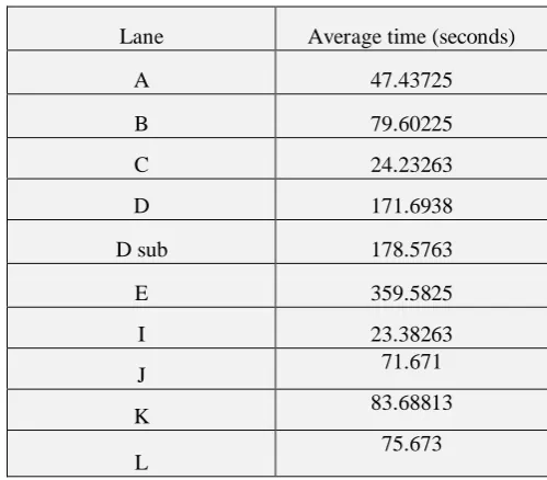
The duration for simulation run was set to two hours, which is the period of peak hours of 5.00 to 7.00 p.m. at Changloon main road. The statistics and the system was initialized between replications. Tables 2 and 3 show the output for all junctions under study.

Table. 2 Average waiting time for basic model

Lane Average time (seconds)

A 47.43725

B 79.60225

C 24.23263

D 171.6938

D sub 178.5763

E 359.5825

I 23.38263

J 71.671

K 83.68813

L 75.673

Table. 3Average number in queue for basic model

Lane

Average number in queue

A 10

B 2

C 3

D 5

D sub 5

E 25

I 7

J 16

K 8

L 4

Model experimentation

Three experiments have been conducted, and each of these experiments is called a scenario. All these scenarios were designed based on suggestion from local people, in-formal interview with staff from Public Works Department, and common sense, which lead to several hypotheses. Those hypotheses were then becoming the foundation for each scenario design. Based on the observation, at certain time, the vehicles from junction 1 are often stuck due to road traf-fic bottleneck. The experimentations were conducted based on the preference to improve this problem. In the following sub-section, several scenarios will be discussed.

Scenario 1

The first scenario was designed by eliminate the barrier from junction 1. Removing the barrier means vehicle from lane B and lane D sub can proceed to respective exit points without having to travel for the extra distance. The move-ment for vehicle from lane D sub was also expected to be smoothed without getting interfered by occupied space.

Scenario 2

The second scenario was designed based on scenario 1. Since there was a significant improvement in total average waiting time, the model from the first scenario became the current model to be further experimented. By making the duration of green light signal at lane I longer, it can improve the road traffic condition. Initially, the green light timing configuration for lane I was set to 57 seconds. For this sce-nario, the green light duration was extended to 80 seconds.

Scenario 3

For the third scenario, it was designed also based on the first scenario. The difference from the second experiment was instead of just only altering the timing configuration for lane I, the timing configuration for lane A and lane E were also being manipulated.

Output analysis

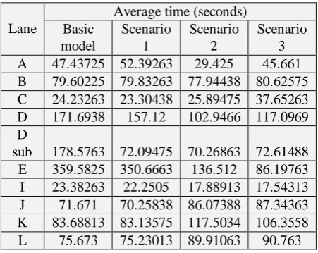
The results obtained from the simulation run for all sce-narios were compared. Table 4 presents the comparison of average waiting time, whereas Table 5 show the comparison of average number in queue for all three scenarios, respec-tively.

Table. 4Comparison of average waiting times for all scenarios

Lane

Average time (seconds) Basic

model

Scenario 1

Scenario 2

Scenario 3

A 47.43725 52.39263 29.425 45.661

B 79.60225 79.83263 77.94438 80.62575 C 24.23263 23.30438 25.89475 37.65263

D 171.6938 157.12 102.9466 117.0969

D

sub 178.5763 72.09475 70.26863 72.61488

E 359.5825 350.6663 136.512 86.19763

I 23.38263 22.2505 17.88913 17.54313

J 71.671 70.25838 86.07388 87.34363

K 83.68813 83.13575 117.5034 106.3558

L 75.673 75.23013 89.91063 90.763

In comparison between basic model and all scenarios, there are not much improvement for average waiting time except for lanes D and D sub. As an example, for lane D, average of 8 replications for average waiting time reduces from 171.69 s to 157.12 s for scenario 1, 102.95 s for sce-nario 2, and 117.10 s for scesce-nario 3. On the other hand, for lane D sub which gives more significant reductions, average waiting time reduces from 178.58 s to 72.09 s for scenario 1, 70.27 s for scenario 2, and 72.61 s for scenario 3. The other significant improvement can be seen in scenario 2 with lane A average waiting time reduces from 47.44 s to 29.43 s and lane E average waiting time reduces from 359.58 s to 136.51 s. However, this improvement comes with trade-off of in-creased average times at lanes J, K, and L.

Table. 5 Comparison of average number in queue for all scenarios

Lane

Average number in queue Basic

model

Scenario 1

Scenario 2

Scenario 3

A 10 10.625 5.75 9

B 2 2.375 1.875 2

C 3 3.25 3.875 5.375

D 5 4 2.625 2.875

D sub 5 2 2 2

E 25 25.375 9.875 6.375

I 7 6.75 5.375 5.375

J 16 14.75 18.5 18.625

K 8 7.75 11.375 10.125

L 4 4.125 5.25 5.125

Similar pattern of improvement also happens for average number in queue comparison between basic model and all scenarios. From Table 5, for example, average number of queue for lane D sub reduces from 5 to 2 for all scenarios. In addition, significant reduction of number in queue for sce-narios 2 and 3 can been seen for lane E, with 25 decreases to 9.88 and 6.38 respectively.

V. CONCLUSION

International Journal of Innovative Technology and Exploring Engineering (IJITEE) ISSN: 2278-3075, Volume-8 Issue-5S March, 2019

Acknowledgement

This research is funded by Universiti Utara Malaysia un-der Geran Penjanaan with S/O Code 13411.

REFERENCES

1. Ismail R, Hafezi MH, Nor RM & Ambak K (2012), Passengers prefer-ence and satisfaction of public transport in Malaysia, Australian Jour-nal of Basic and Applied Sciences 6, 410–416.

2. Road Transport Department Malaysia (2015), Total Vehicle Registra-tion Based on Year, available on line: http://www.jpj.gov.my

3. Ferreira M, Fernandes R, Conceição H, Viriyasitavat W & Tonguz OK (2010), Self-organized traffic control, Proceedings of the seventh ACM international workshop on VehiculAr InterNETworking-VANET’10 4. Kamrani M, Hashemi Esmaeil Abadi SM & Rahimpour Golroudbary S

(2014), Traffic simulation of two adjacent unsignalized T -junctions during rush hours using Arena software, Simulation Modelling Practice and Theory, 49, 167–179.

5. Qi L, Zhou M & Luan W (2018), A Two-level Traffic Light Control Strategy for Preventing Incident-Based Urban Traffic Congestion, IEEE Transactions on Intelligent Transportation Systems, 19, 13–24. 6. Sánchez-Medina JJ, Galán-Moreno MJ & Rubio-Royo E (2010),

Traf-fic signal optimization in la Almozara District in Saragossa under con-gestion conditions, using genetic algorithms, traffic microsimulation, and cluster computing, IEEE Transactions on Intelligent Transportation Systems, 11, 132–141.

7. Yousef KM, Al-Karaki JN & Shatnawi AM (2010), Intelligent Traffic Light Flow Control System Using Wireless Sensors Networks, Infor-mation Science and Engineering, 26, 753–768.

8. Barrachina J, Garrido P, Fogue M, Martinez FJ, Cano JC, Calafate CT & Manzoni P (2012), D-RSU: a density-based approach for road side unit deployment in urban scenarios, International workshop on ipv6-based vehicular networks (Vehi6), collocated with the 2012 IEEE intel-ligent vehicles symposium, 1–6.

9. Kok AL, Hans EW & Schutten JMJ (2012), Vehicle routing under time-dependent travel times: The impact of congestion avoidance, Computers and Operations Research, 39, 910–918.

10.Jain V, Sharma A & Subramanian L (2012), Road traffic congestion in the developing world, Proceedings of the 2nd ACM Symposium on Computing for Development - ACM DEV ’12.

11.Downie A (2008), The World’s Worst Traffic Jams, Time Magazine,

available on line:

http://content.time.com/time/world/article/0,8599,1733872,00.html 12.Su B, Huang H & Li Y (2016), Integrated simulation method for

water-logging and traffic congestion under urban rainstorms, Natural Hazards, 81, 23–40.

13.Huang Y, Weng Y & Zhou M (2014), Modular Design of Urban Traf-fic-Light Control Systems Based on Synchronized Timed Petri Nets, IEEE Transactions on Intelligent Transportation Systems, 15, 530–539. 14.Tan KK, Khalid M & Yusof R (1996), Intelligent traffic lights control

by fuzzy logic, Malaysian Journal of Computer Science, 9, 29–35. 15.Adam I, Wahab A, Yaakop M, Salam AA & Zaharudin Z (2014),

Adaptive Fuzzy Logic Traffic Light Management System, 4th Interna-tional Conference on Engineering Technology and Technopreneuship, 340–343.

16.Hewage KN & Ruwanpura JY (2004), Optimization of traffic signal light timing using simulation, Proceedings - Winter Simulation Confer-ence, 2, 1428–1433.

17.Maidstone R (2012), Discrete Event Simulation, System Dynamics and Agent Based Simulation: Discussion and Comparison, System, 1–6. 18.Nawawi MKM, Jamil FC & Hamzah FM (2015), Evaluating

perfor-mance of container terminal operation using simulation, AIP Confer-ence Proceedings, 1660.