Up-to-date mathematical models lines of
development of information technologies in the
field of numerical methods of structures
strength calculations
Vladimir Meleshko1
1 Saint Petersburg State University of Architecture and Civil Engineering, Faculty of civil
engineering, 190005 2-ya Krasnoarmeiskaya st. 4, Russian Federation
Abstract. In order to carry out reliable calculations of structures adequate to reality, in particular, for taking into account plastic resource, it is necessary to use complex program systems and build finite element models of high dimensionality. This work provides a comparison of different mathematical models, which can be used for numerical analysis. Consideration was given to basic variation principles and methods of calculating structural mechanics. Distinctive features of forming systems of equations of classical methods of structural mechanics and known numerical methods were demonstrated. Possible advantages of methods with respect to accuracy and rate of calculations were revealed. Consideration was given to possible improvements of existing mathematical models in elastoplastic domain. Possible directions of development in the field of engineering methods for calculating strength were proposed.
1 Introduction
The information technologies, which rapid development makes it possible to essentially expand the instrument base of investigations in different fields, play an important role in modern construction. The structures of greater complexity are used more and more frequently, in the wake of developing trends characterizing a process of architectural creative work. The work under extreme conditions, efficient use of new materials, all this determines a necessity of development of more efficient approaches to calculation of structures proper, being based on up-to-date tools, in which development the key role belongs to innovative mathematical models and derivatives to product programs.
A permanent improvement of structures and equipment brings the development of existing calculation methods of mechanics to the first place. A considerable amount of time has passed since the emergence of finite-elements method, during which it has succeeded to prove itself as a universal method for solving tasks of mechanics, gas-dynamics and electrical engineering. Nevertheless, there exist narrow opportunities of improving the
method of finite elements in separate domains. The improvements resolve basically into application of modern algorithms of calculating systems of equations, improving a process of repeatability. The improvement can manifest itself in accuracy and rate of calculation and can be performed in elastoplastic domain, if it can not be performed in the elastic domain.
The improvement of the existing methods of numerical analysis resolve itself into different hybrid wordings, which associate analytical expressions with numerical methods and solving integral equations, which brings about a reduction of unknown degrees of freedom.
The purpose of this work consists in revealing peculiarities of different methods of construction mechanical equipment for optimization of calculations of elastoplastic deformations.
2 Methods of Solving Problems of Construction Mechanical
Equipment
2.1 Classical methods
Let us give consideration to classical methods of structural mechanics: force method, displacement method and mixed method. The classical methods of structural mechanics are described quite in details in equation [1]. The first two have been obtained on the basis of variation Lagrange and Castigliano principle [2, 3]. The mixed method presents a combination of method of forces and displacements. A variation Reissner principle corresponds to this method. The meaning of mixed method consists in the fact that different parts of trussed system can have different degrees of static and kinematic non-definability. Discriminating the least degree in every part of trussed system, it is possible to optimize the system of canonical equations making it mixed, i.е. consisting of unknown displacements and forces and, thus, reduce the number of equations in the system.
The canonical equations of classical methods get received through selection of the main system, which characterizes continuous function in corresponding composed functions of potential energy. This continuous function is expressed through unknown displacements of kinematically definable system or efforts in the discarded links of statically non-definable system. For instance, a system of canonical equations for the method of displacements looks as follows:
0 0
1 1
1 1 1 11
nP n nn n
P n n
R u r u r
R u r u r
, (1)
where, rij– rigidity factors; ui– unknown displacements.
Let us present equations (1) in a matrix form
R
u P (2)
nn n
n
r r
r r
R
1 1 11
(3)
TnP
P R
R
method of finite elements in separate domains. The improvements resolve basically into application of modern algorithms of calculating systems of equations, improving a process of repeatability. The improvement can manifest itself in accuracy and rate of calculation and can be performed in elastoplastic domain, if it can not be performed in the elastic domain.
The improvement of the existing methods of numerical analysis resolve itself into different hybrid wordings, which associate analytical expressions with numerical methods and solving integral equations, which brings about a reduction of unknown degrees of freedom.
The purpose of this work consists in revealing peculiarities of different methods of construction mechanical equipment for optimization of calculations of elastoplastic deformations.
2 Methods of Solving Problems of Construction Mechanical
Equipment
2.1 Classical methods
Let us give consideration to classical methods of structural mechanics: force method, displacement method and mixed method. The classical methods of structural mechanics are described quite in details in equation [1]. The first two have been obtained on the basis of variation Lagrange and Castigliano principle [2, 3]. The mixed method presents a combination of method of forces and displacements. A variation Reissner principle corresponds to this method. The meaning of mixed method consists in the fact that different parts of trussed system can have different degrees of static and kinematic non-definability. Discriminating the least degree in every part of trussed system, it is possible to optimize the system of canonical equations making it mixed, i.е. consisting of unknown displacements and forces and, thus, reduce the number of equations in the system.
The canonical equations of classical methods get received through selection of the main system, which characterizes continuous function in corresponding composed functions of potential energy. This continuous function is expressed through unknown displacements of kinematically definable system or efforts in the discarded links of statically non-definable system. For instance, a system of canonical equations for the method of displacements looks as follows:
0 0 1 1 1 1 1 11 nP n nn n P n n R u r u r R u r u r
, (1)
where, rij– rigidity factors; ui– unknown displacements.
Let us present equations (1) in a matrix form
R
u P (2)
nn n n r r r r R 1 1 11 (3)
TnP
P R
R
P 1 (4)
Tn
u u
u 1 (5)
The main drawback when compiling equations in these methods is a selection of the main system, which complicates the process of automation and, accordingly, integration into program complexes.
2.2 Numerical Methods of Calculation
Let us further give consideration to the known approximation methods, such as Ritz method, method of weighted residuals (minimization of residual errors, errors, in particular, Bubnov-Galerkin method and variation-difference method.
The idea of Ritz method consists in that a finite number of basic functions ͳ, ʹ, … , is selected and a combination providing minimum of composed function is looked for among all linear combinations of ui type. It is Ritz approximation [4, 5, 6]. The unknown coefficients ui are determined already not from differential equations, but from
system n of discrete algebraic equations, for solution of which it is possible to use computer. In other words, we change from continual problem with an endless number of degrees of freedom with respect to the form of body deformation we turn to the problem for a system with a finite number of degrees of freedom. The theoretical substantiation of this method is very simple: minimization process automatically gives a combination nearest to function y(x). Thus, the purpose consists in selecting the basis functions , taking into account boundary constraints quite convenient for calculation and minimization of potential energy and at the same time provide for good approximation of unknown solution y(x).
Let us review a composed function of full potential energy for the trussed system [7].
W U
П (6)
The approximation Ritz method consists in direct minimization of full potential energy of system П. Let us set the change of displacements as the following function
) x ( f u ) x (
y n i
i i
1
, (7)
Then dx ) x ( f u EI dx ) x ( y EI W l i n i i l
0 2 1 0 2 2 2 (8) dx ) x ( f u ) x ( p dx ) x ( y ) x ( p U l i n i i l
0 1 0 (9)Let us substitute (8) and (9) in (6) and differentiate according to ui.
dx ) x ( f ) x ( f u EI dx ) x ( f ) x ( p u П k l i n i i l n i i i
0 1
0 1 2
The first variation of full potential energy equals zero (condition of potential energy stationary state) on the basis of variation Lagrange principle. As a result, we obtain n of equations
0
i i
i u
W u U u
П . (11)
These equations form a system of algebraic linear equations (1) with respect to generalized displacements ui in case of linearly deformable system with due account of
equation (10).
Let us apply Ritz method in the variational formulation of Castigliano. Let us review statically undeterminable beam on two supports. There exists an infinite aggregate of equilibrium bending-moment curves set by the equality
1 1M
X M
M P , (12)
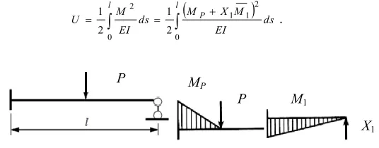
where, МP and M1 are the bending-moment curves (Fig. 1), while Х1 is an arbitrary variate
of bearing reaction.
The Castigliano principle in an integral form expresses conditions of compatibility of body deformations and zero equality of the first variation of potential energy. Let us find Х1 using a principle of least work (physical entity of Castigliano principle). The deformation energy taking into account bending moments only will equal:
l P l
ds EI
M X M ds EI M U
0
2 1 1
0 2
2 1 2
[image:4.482.117.385.317.422.2]1 . (13)
Fig. 1. Beam on two supports and moment curves.
A condition of minimum of deformation energy U according to Castigliano gives:
0
0 1 1
0 2 1 1
l P l
ds EI
M M X ds EI M X
U
. (14)
Let us present integral equations in the form of
l
ds EI M
0 2 1
11 , (15)
l P P MEIM ds
0 1
1 . (16)
As a result we will get a known equation for solution of statically undeterminable systems by the method of forces expressing a zero equality of deflection at pivot bearing
0 1 1 11
X P . (17)
P P
X1 M1
The first variation of full potential energy equals zero (condition of potential energy stationary state) on the basis of variation Lagrange principle. As a result, we obtain n of equations 0 i i i u W u U u
П . (11)
These equations form a system of algebraic linear equations (1) with respect to generalized displacements ui in case of linearly deformable system with due account of
equation (10).
Let us apply Ritz method in the variational formulation of Castigliano. Let us review statically undeterminable beam on two supports. There exists an infinite aggregate of equilibrium bending-moment curves set by the equality
1 1M
X M
M P , (12)
where, МP and M1 are the bending-moment curves (Fig. 1), while Х1 is an arbitrary variate
of bearing reaction.
The Castigliano principle in an integral form expresses conditions of compatibility of body deformations and zero equality of the first variation of potential energy. Let us find Х1 using a principle of least work (physical entity of Castigliano principle). The deformation energy taking into account bending moments only will equal:
l P l ds EI M X M ds EI M U 0 2 1 1 0 2 2 1 21 . (13)
Fig. 1. Beam on two supports and moment curves.
A condition of minimum of deformation energy U according to Castigliano gives:
0 0 1 1 0 2 1 1
l P l ds EI M M X ds EI M X U. (14)
Let us present integral equations in the form of
l ds EI M 0 2 111 , (15)
l P P MEIM ds
0 1
1 . (16)
As a result we will get a known equation for solution of statically undeterminable systems by the method of forces expressing a zero equality of deflection at pivot bearing
0 1 1 11
X P . (17)
P P
X1 M1
MP
Let us consider statically undeterminable trussed system n times and select the undefined efforts such that the system remains geometrically invariable. Let us present the moment in the form of a function:
n
i i i
M X M
M P
1 . (18)
Having calculated the potential energy U(Xi, P) (i = 1,2,….n), on the basis of
Castigliano variation principle:
0 1
i n i i X X UU . (19)
In view of arbitrariness of variations Xi, we will get n of equations of forces method
0 i X
U , (20)
or in detail:
0 0 1 1 1 1 1 11 nP n nn n P n n X X X X
. (21)
Let us give brief consideration to the following two methods. The variation-difference method makes it possible to confine solution of differential equations for continuous functions to numerical solution of a system of algebraic equations in the way of difference approximation of derivatives in a composed function. As a result of solving such task, it becomes possible to determine the values of the sought-for function in the finite number of points. The idea of method of weighted residuals is based on selecting a solution. The method is based on the requirement of orthogonal origin of functions to a residual error. If a residual error equals zero, it is orthogonal to a fundamental system of functions. Let us set forth an approximated solution in the following form:
) x ( f u ) x ( ) x (
y~ n i
i i
1, (22)
at that, function (x) positively meets boundary conditions, while basis functionsfi (x)
assume zero value at the boundary. Let us introduce a residual error or an error ) x ( y~ ) x ( y
R . (23)
In order to minimize a residual error
0
dR , (24)
But in this case (with n > 1) after expansion of integral equation we arrive at incomplete system of equations with respect to ui. Since we want that the residual error equals zero
(R 0), multiplying of the residual error by some function shall not change a value of integral equation, i.e.
0
d
R
Wk , (25)
where, Wk are the weight functions.
When i = 1, 2, …, n we will arrive at incomplete system of equations with respect to coefficients ui. The peculiarity of Bubnov-Galerkin method consists in the fact that basis
functions are aссepted as the weight functions.
All these methods are based on the fact that the approximating function is continuous. Based thereupon we obtain a definite system of equations with respect to indefinite approximation coefficients. The following two methods make it possible to present a solution in the form of piecewise continuous function.
2.3 Finite Elements Method
The finite elements method (FEM) is a powerful tool of approximated direct finding of unknown functions on the basis of any variation principle in elasticity and structural theory problems. It can be interpreted as a specific form of Ritz method, which provides a key for theoretical substantiation.
There are several FEM versions: direct method, variation method, residual method and energy balance method; and there are several FEM forms: displacement method, force method and mixed method [8, 9, 10, 11]. In order to reveal the key peculiarities and differences from Ritz method, let us give more detailed consideration to variation FEM in the form of displacements method.
FEM can be described in a couple of words. Let the task to be solved is set in a variation form: it is necessary to find function u(x, y, z) minimizing the set composed function of potential energy. The composed function of energy is presented here for the entire region under consideration in the form of a sum of composed functions of its separate parts – finite elements. A dedicated law of distributing the sought-for functions is specified for the region of every element independently from the other ones. Such a piecewise continuous approximation will be made by means of specifically selected approximating functions, also referred to as coordinate functions or interpolating functions. They are used to express the sought-for continuous values (displacements, strains, etc.) within the limits of every FE through the figures of these values in nodal points, while an arbitrary preset load gets replaced with a system of equivalent nodal forces.
A difficulty of applying Ritz method consists in that it is practically impossible to select such a system of basis functions fi(х, у, z) for the intricate-shaped solid, which being set within entire field of the region, would take into account different local peculiarities of its stress and strain state. The finite elements method eliminates this basic difficulty by introducing piecewise continuous functions, which equal zero everywhere, except for limited sub-regions, which are the finite elements. As a result, the matrix of coefficients of resolving system of equations it assumes a banded unloaded structure.
But in this case (with n > 1) after expansion of integral equation we arrive at incomplete system of equations with respect to ui. Since we want that the residual error equals zero
(R0), multiplying of the residual error by some function shall not change a value of integral equation, i.e.
0
d
R
Wk , (25)
where, Wk are the weight functions.
When i = 1, 2, …, n we will arrive at incomplete system of equations with respect to coefficients ui. The peculiarity of Bubnov-Galerkin method consists in the fact that basis
functions are aссepted as the weight functions.
All these methods are based on the fact that the approximating function is continuous. Based thereupon we obtain a definite system of equations with respect to indefinite approximation coefficients. The following two methods make it possible to present a solution in the form of piecewise continuous function.
2.3 Finite Elements Method
The finite elements method (FEM) is a powerful tool of approximated direct finding of unknown functions on the basis of any variation principle in elasticity and structural theory problems. It can be interpreted as a specific form of Ritz method, which provides a key for theoretical substantiation.
There are several FEM versions: direct method, variation method, residual method and energy balance method; and there are several FEM forms: displacement method, force method and mixed method [8, 9, 10, 11]. In order to reveal the key peculiarities and differences from Ritz method, let us give more detailed consideration to variation FEM in the form of displacements method.
FEM can be described in a couple of words. Let the task to be solved is set in a variation form: it is necessary to find function u(x, y, z) minimizing the set composed function of potential energy. The composed function of energy is presented here for the entire region under consideration in the form of a sum of composed functions of its separate parts – finite elements. A dedicated law of distributing the sought-for functions is specified for the region of every element independently from the other ones. Such a piecewise continuous approximation will be made by means of specifically selected approximating functions, also referred to as coordinate functions or interpolating functions. They are used to express the sought-for continuous values (displacements, strains, etc.) within the limits of every FE through the figures of these values in nodal points, while an arbitrary preset load gets replaced with a system of equivalent nodal forces.
A difficulty of applying Ritz method consists in that it is practically impossible to select such a system of basis functions fi(х, у, z) for the intricate-shaped solid, which being set within entire field of the region, would take into account different local peculiarities of its stress and strain state. The finite elements method eliminates this basic difficulty by introducing piecewise continuous functions, which equal zero everywhere, except for limited sub-regions, which are the finite elements. As a result, the matrix of coefficients of resolving system of equations it assumes a banded unloaded structure.
A physical problem definition corresponds, as a rule, to a certain structure with the loads applied thereto. The idealization of physical problem definition and further acquisition of mathematic model there from contemplates availability of assumptions, which all together bring about a system of differential equations corresponding to mathematical formulation of the problem.
If the task is being solved in displacements, i.e., their values are set at the boundaries, the potential system energy shall be minimized. If the task is being solved in stresses, while the external loads are set at the boundaries, an additional system operation will be minimized.
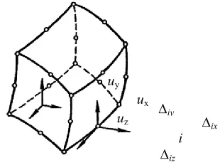
An assumption is made in the finite elements method, according to which the displacements of all element points get expressly determined by its nodal displacements (Fig. 2)
ue
N
e , (26)
Tz y x
e u u u
u , (27)
Tj i
e
, (28)
Tiz iy ix
i
, (29)
where, [N] is a rectangular matrix, where the quantity of lines equals the number of components u, while the number of columns corresponds to a number of vector
[image:7.482.193.348.299.415.2]components. The approximating coordinate functions are the matrix elements.
Fig. 2. Element displacements.
Let us express deformations in every point of finite element using Cauchy geometrical relationships [6] through its nodal displacements
e
D
ue , (30)
e
D N
e . (31)Let us present [N] in such a form
Tz y
x N N
N
N , (32)
where, Nx, Ny, Nz are the matrices of a line, where the known approximating functions are
its elements.
uy
uz ux
iy ix
z N x
N z
N y N
y N x N z
Ny Nx N
N N N
x z
y z x y
z y x
N D A
x z
y z
x y
z y x
z y x
0 0
0 0 0
0 0
0 0
. (33)
Let us put down Hooke's law in such a form
e
с
e , (34)where,
e is a vector of stresses; [c] is an elastic-constant matrix. Let us substitute (30)and (32) in (33), then
e
c A
e . (35)It is seen from the obtained relations that the stress and strain state of finite element will be expressly determined by nodal displacements with the known function of approximating functions [N].
If the received interrelations are substituted into composed function for full potential energy and summarized for every finite element, after minimization of cumulative composed function taking into account boundary conditions we will get a system of FEM resolving equations
P
k , (36)
k
AT c AdVV
e
, (37)where, k is a matrix of system rigidity; keis a matrix of finite-element rigidity.
In order to solve simultaneous linear algebraic equations (SLAE), both the exact and (with high system order) iteration methods are used. The effective numerical procedures built thereupon take into account symmetry and banded structure of system rigidity matrix.
2.4 Boundary-Element Method
FEM helps to solve the tasks of calculating different trussed and continual systems. An extensive experience of using FEM has revealed not only the advantages of this method, but the expressed drawbacks too, which can be eliminated on the basis of fundamentally new approaches, e.g., the theories of integral equations in the boundary-element method (BEM). The methods of solving boundary value problems on the basis of integral equations are considered more exact and economical than the methods based on approximation of differential operators (FEM).
z N x N z N y N y N x N z Ny Nx N N N N x z y z x y z y x N D A x z y z x y z y x z y x 0 0 0 0 0 0 0 0 0. (33)
Let us put down Hooke's law in such a form
e
с
e , (34)where,
e is a vector of stresses; [c] is an elastic-constant matrix. Let us substitute (30)and (32) in (33), then
e
c A
e . (35)It is seen from the obtained relations that the stress and strain state of finite element will be expressly determined by nodal displacements with the known function of approximating functions [N].
If the received interrelations are substituted into composed function for full potential energy and summarized for every finite element, after minimization of cumulative composed function taking into account boundary conditions we will get a system of FEM resolving equations
P
k , (36)
k
AT c AdVV
e
, (37)where, k is a matrix of system rigidity; keis a matrix of finite-element rigidity.
In order to solve simultaneous linear algebraic equations (SLAE), both the exact and (with high system order) iteration methods are used. The effective numerical procedures built thereupon take into account symmetry and banded structure of system rigidity matrix.
2.4 Boundary-Element Method
FEM helps to solve the tasks of calculating different trussed and continual systems. An extensive experience of using FEM has revealed not only the advantages of this method, but the expressed drawbacks too, which can be eliminated on the basis of fundamentally new approaches, e.g., the theories of integral equations in the boundary-element method (BEM). The methods of solving boundary value problems on the basis of integral equations are considered more exact and economical than the methods based on approximation of differential operators (FEM).
As compared with FEM, BEM can exceed the existing methods with respect to accuracy and authenticity of the results by duration of processor operation and memory footprint.
[image:9.482.124.358.144.230.2]The substance of BEM consists in solution of potential Laplace and Poisson equations with different boundary conditions (Dirichlet, Neumann, Robin) using integral Gauss-Greene and Gauss-Ostrogradsky transformations, under condition of boundary discretization by the finite number of segments, which are referred to as the boundary elements (Fig. 3).
Fig. 3. Discretization of boundaries and region .
Let us put down the potential theory main equation, in particular, in case of bidimensional problem [12]
2u f(x,y) x,y , (38)
where, 2 is a Laplace operator or harmonic operator. It will be determined in the following way: 2 2 2 2 2 y x x j x i x j x i
. (39)
Equation (1) in case of f = 0 is referred to as Laplace equation, and in case of f 0 – as Poisson equation. Its solution u = u(x, y) presents a potential determined in point (x, y) of region of source function f(x, y) distributed to . The solution shall meet the task boundary conditions at boundary Г. The boundary problems (Dirichlet, Neumann, Robin and mixed problem) for potential equation can be joined by consolidated wording
Г , n u u , f u 2
, (40)
where,
y n x n x j x i j n i n nn x y x y
. (41)
is an operator, which differentiates the scalar function in direction n; = (s), = (s) and
= (s) are known functions defined at boundary Г.
Every of four boundary problems can be obtained from equation (3) by means of corresponding identification of functions , , [12]. Equation (4) is referred to as the second Green identity for harmonic operator. The fundamental and numerical solution of these equations is presented in [12].
The issues of theory and practical application of BEM numerical and analytical variant with respect to unidimensional structural models of linear truss and plate systems are considered in [13, 14].
The basic advantage of BEM is an exact compliance with the initial differential equation inside of computational domain. In the problems with infinite boundary BEM
Nodes
features an advantage due to the ease of its accountability. A completely filled matrix of the resulting simultaneous linear algebraic equations (SLAE) can be attributed to method drawbacks unlike the loose (unloaded) one in BEM, where it comprises a great number of zeroes. Since the mesh is applied to the region boundary only, the matrix dimensionality will be the next lower order, than with BEM. In case of solving integral equations analytically a presence of flat boundary is necessary, since the singular integrals do not exist in angular points of piecewise-smooth boundary.
3 Conclusion
It proceeds from the above that presently the finite-elements method in classical form is not exclusion for solving mechanics problems and in many cases it can be irrational. For instance, an alternative method of boundary elements makes it possible to reduce the number of equations by an order of magnitude using numerical integration across the region and discretization across the boundary. In case the trussed systems are given consideration in elastoplastic domain, the finite-elements method in the form of forces method can increase the accuracy of determining internal efforts. In case of using generalized formula of Mohr [15] it is possible not to divide rods into finite elements. In such case the order of system of equations for long rods can be reduced significantly.
There is an extensive scope of functions, in which structural models are used with a great number of degrees of freedom. It increases time of numerical calculation as a result of exponential dependence on the number of resulting BEM equations unknown in the system. In order to optimize expenditures, a plastic resource is considered most frequently in many problems, which brings about a more reasonable material utilization. The operation of construction structures takes place not infrequently under extreme conditions, where the existing linear approaches are not always justified and it is necessary to take into account the non-linear behavior of structures. All this results in definite complications in the course of designing.
In spite of the fact that BEM has proven itself well in the elastic zone, the problems with a great number of degrees of freedom and the problems related to determining elastoplastic deformations feature possibilities for the development of existing methods. Hence, one can make a conclusion on a possibility of development of additional wordings for particular problems, and elastoplastic, in particular.
References
1. А.V. Darkov, N.N. Shaposhnikov, Structural Mechanics (Publishing house Vysshaya shkola, Moscow, 1986)
2. V.I. Slivker, Structural Mechanics. Variation Basics (Publishing house ASV, Moscow, 2005)
3. K. Vasidzu, Variation Methods in the Theory of Elasticity and Plasticity (Publishing house Mir, Moscow, 1987)
4. N.S. Bakhvalov, N.P. Zhidkov, G.М. Kobelkov, Numerical Methods (Nauka, Moscow, 1987)
5. V.P. Ilyin, V.V. Karpov, А.М. Maslennikov, Numerical Methods of Solving Problems of Structural Mechanics (Vysheishaya shkola, Minsk, 1990)
6. V.I. Samul’, Fundamentals of Theory of Elasticity and Plasticity (Vysshaya shkola, Moscow, 1982)
7. А.V. Ignatiev, Vestnik MGSU, 1(3) (2015)
8. М. Sekulovich, Finite Elements Method (Stroyizdat, Moscow, 1993)
9. I. N. Serpik, Finite Elements Method in Solving Problems of Mechanics of Carrier Systems (Publishing house АSV, Moscow, 2015)
10. R. Gallaher, Finite Elements Method. Fundamentals (Publishing house Mir, Moscow, 1984)
11. S.I. Trushi, Finite Elements Method. Theory and Problems (Publishing house of Association of construction HEI, Moscow, 2008)
12. J. Katsikadelis, Boundary Elements. Theory and Applications (Publishing house АSV, Moscow, 2015)
13. V.А. Bazhenov, V.F. Orobei, А.F. Dashchenko, L.V. Kolomiets, Structural Mechanics. Special Course. Application of Boundary Elements Method (Astroprint, Odessa, 2001) 14. P. Benardji, R. Batterfield, Boundary Elements Method in Applied Sciences (Mir,
Moscow, 1984)