Semidiurnal solar tide differences between fall and spring transition times in the Northern Hemisphere

https://doi.org/10.5194/angeo-36-999-2018 © Author(s) 2018. This work is distributed under the Creative Commons Attribution 4.0 License.

Semidiurnal solar tide differences between fall and spring transition

times in the Northern Hemisphere

J. Federico Conte1, Jorge L. Chau1, Fazlul I. Laskar1, Gunter Stober1, Hauke Schmidt2, and Peter Brown3

1_{Leibniz Institute of Atmospheric Physics, University of Rostock, Kühlungsborn, Germany} 2_{Max Planck Institute for Meteorology, Hamburg, Germany}

3_{Department of Physics and Astronomy, Western University, London, Ontario, Canada}

Correspondence:J. Federico Conte ([email protected]) Received: 29 March 2018 – Discussion started: 3 April 2018

Revised: 27 June 2018 – Accepted: 5 July 2018 – Published: 13 July 2018

Abstract. We present a study of the semidiurnal solar tide (S2) during the fall and spring transition times in the North-ern Hemisphere. The tides have been obtained from wind measurements provided by three meteor radars located at Andenes (69◦N, 16◦E), Juliusruh (54◦N, 13◦E) and Tavi-stock (42◦N, 81◦W). During the fall, S2 is characterized by a sudden and pronounced decrease occurring every year and at all height levels. The spring transition also shows a de-crease in S2, but not sudden and that ascends from lower to higher altitudes during an interval of ∼15 to 40 days. To assess contributions of different semidiurnal tidal com-ponents, we have examined a 20-year free-run simulation by the Hamburg Model of the Neutral and Ionized Atmo-sphere (HAMMONIA). We found that the differences exhib-ited by the S2 tide between equinox times are mainly due to distinct behaviors of the migrating semidiurnal and the non-migrating westward-propagating wave number 1 tidal components (SW2 and SW1, respectively). Specifically, dur-ing the fall both SW2 and SW1 decrease, while durdur-ing the springtime SW2 decreases but SW1 remains approximately constant or decreases only slightly. The decrease shown by SW1 during the fall occurs later than that of SW2 and S2, which indicates that the behavior of S2 is mainly driven by the migrating component. Nonetheless, the influence of SW1 is necessary to explain the behavior of S2 during the spring. In addition, a strong shift in the phase of S2 (of SW2 in the simulations) is also observed during the fall. Our meteor radar wind measurements show more gravity wave activity in the fall than during the spring, which might be indicating that the fall decrease is partly due to interactions between SW2 and gravity waves.

1 Introduction

It is well known that the mesosphere and lower thermosphere (MLT) variability is strongly influenced by a large variety of waves that dynamically interact and couple different re-gions of the terrestrial atmosphere. Global-scale waves in-clude planetary waves (PWs), which have periods of∼2– 30 days, as well as thermal tides, which have periods that are harmonics of the solar day (e.g., Rossby, 1939; Forbes, 1984). Gravity waves (GWs), on the other hand, are local-scale waves characterized by shorter vertical wavelengths and periods of minutes to a few hours (e.g., Fritts and Alexan-der, 2003). Thermal tides are mainly excited by solar heating of water vapor and ozone. Due to the excitation processes, the dominant tidal components have periods of one solar day (24 h) and its two first harmonics, i.e., 12 and 8 h. When the tides propagate Sun-synchronously, they are identified as mi-grating. The non-migrating tides are primarily excited by tro-pospheric latent heat release and may be westward or east-ward propagating (Hagan and Forbes, 2002, 2003). Another source of non-migrating tides is the non-linear interaction be-tween migrating tides and stationary planetary waves (e.g., Angelats i Coll and Forbes, 2002).

1000 J. F. Conte et al.: Semidiurnal solar tide variability

Charlton and Polvani, 2007; Fuller-Rowell et al., 2010). The spring and fall transitions also show strong changes in the mean winds (e.g., Shepherd et al., 1999; Taylor et al., 2001; Matthias et al., 2015). Hence, one may expect an enhanced and different response of the tides during these time intervals. Previous studies have investigated the behavior of solar tides during equinox times (e.g., Riggin et al., 2003; Pancheva et al., 2009). More recently, Chau et al. (2015) reported a per-sistent and sudden decrease in the semidiurnal solar tide (S2) in the Northern Hemisphere during the September and Oc-tober months. However, they did not provide an explanation of this observed sharp decrease in S2. Laskar et al. (2016) speculated that the enhanced S2 amplitudes observed during August and September over Andenes (northern Norway) and Juliusruh (northern Germany) might be due to phase in-teraction between the migrating semidiurnal (SW2) and the non-migrating westward-propagating wave number 1 semid-iurnal (SW1) tidal components, but they could not verify this due to a lack of global datasets. Recent studies have also ex-amined the mechanisms of how gravity waves influence so-lar tides in the middle and upper atmosphere (e.g., Yi˘git and Medvedev, 2017). All this motivated us to further investigate the differences in the response of the S2 tide between the spring and fall transition times in the Northern Hemisphere using both observations and model simulations.

The structure of this paper is as follows. In Sect. 2, we present and describe the tidal features in both radar measure-ments and model simulations. Section 3 is used to discuss the comparison of observations with model simulations, in order to explain the differences seen in the behavior of the semidi-urnal solar tide between equinoxes. Conclusions are given in Sect. 4.

2 Results

2.1 Semidiurnal solar tide as measured by meteor radars

Specular meteor radars constitute an excellent tool to study winds in the mesosphere and lower thermosphere region (e.g., Hocking et al., 2001; McCormack et al., 2016). These remote sensing instruments continuously observe winds in the height range extending from∼75 up to 105 km, with a typical vertical resolution of 2 km (e.g., Stober et al., 2017). From these wind measurements, it is possible to extract de-tailed information about the mean winds and tides, as well as planetary waves and gravity waves (e.g., Hocking and Thaya-paran, 1997; Hoffmann et al., 2007).

In this work, we have analyzed wind measurements pro-vided by three meteor radars located at Andenes (69.3◦N, 16◦E), Juliusruh (54.6◦N, 13.3◦E) and Tavistock (42.3◦N, 80.8◦W). The tidal information has been estimated by means of a least square technique. Assuming that the zonal (u) and meridional (v) winds result from the superposition of a mean

wind (U0andV0, respectively) plus oscillations of different

periods, we independently fit the observations in each hor-izontal component with sinusoidal functions of periods Ti

equal to 24, 12 and 8 h in order to account for the diurnal, semidiurnal and terdiurnal solar tides,

(u, v)=(U0, V0)+ 3

X

i=1

A(u,v)icos

2π(t−φ(u,v)i) Ti

, (1)

whereA(u,v)i andφ(u,v)i represent the amplitude and phase, respectively, of the different tidal components. In this way, assuming that the tidal phases are stable within the selected running window, daily values of the mean winds, and the am-plitude and phase of each tide were determined in bins of 21 days shifted by 1 day. Besides, information on the gravity wave activity is provided by the residuals of the fitting pro-cess, since they contain most of the wave-like perturbations different than tides and planetary waves.

It must be noted that from ground-based single-station measurements it is not possible to decompose the observed tides into different wave numbers, which implies that we can-not differentiate between migrating and non-migrating tidal components.

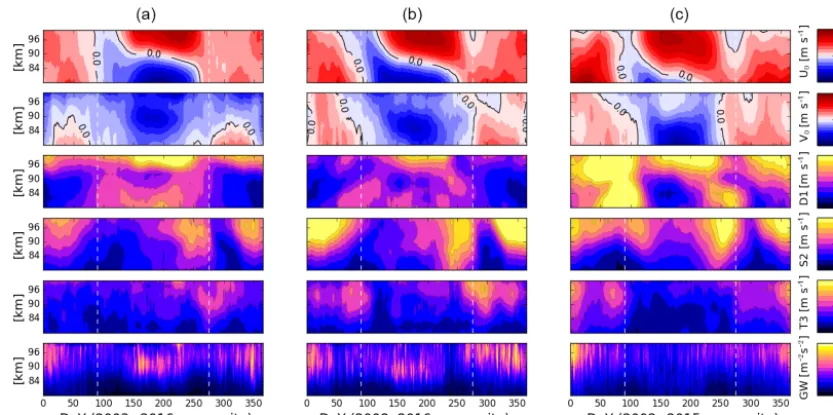
In Fig. 1, we present a composite for the three sites con-sidered in this study of the mean zonal (U0) and meridional

(V0) winds, the total amplitude of the diurnal (D1),

Figure 1. Composites of mean zonal (U0) and meridional winds (V0), diurnal, semidiurnal and terdiurnal solar tides (D1, S2 and T3,

respectively), and GW kinetic energy over (columna) Andenes, (columnb) Juliusruh and (columnc) Tavistock. The vertical white dashed lines indicate DoYs 90 and 275. The composites were determined for the entire yearly datasets available at the time this study was initiated.

decrease is seen every year at the three locations, and extends for a period of∼15 days or more, depending on the year.

The seasonal behavior of the gravity waves is different than that of the S2 tide. From the bottom panels of Fig. 1, it can be seen that GWs show significant activity during the winter at all three locations, but that it is considerable dur-ing summer only over Andenes and Juliusruh. On the other hand, GWs exhibit a clear pattern during equinox times over the three sites: there is more activity during the fall than in the spring. This is clearest over Juliusruh, where an enhance-ment in the GW activity can be seen at approximately the same time the S2 tide abruptly decreases. The terdiurnal so-lar tide has a period of 8 h, which falls almost in the middle of the spectrum of typical GW periods (our measurements allow us to see GWs with periods larger than 2 h). Since the wavelength information was not available for this study, we were not able to decompose the T3 tide into the 8 h tidal wave and the GWs with that same period. Hence, to better assess the GW activity, the T3 tide must be included in the analy-sis. The seasonal variability of T3 presents some similarities with that of the GWs, although the amplitude enhancement seen in the fall at around the same time S2 starts decreasing is more pronounced in the case of T3.

The time of occurrence of the S2 tide fall decrease varies from year to year. This can be deduced from Fig. 2, where we present the annual variability of the semidiurnal solar tide during the period 2008–2015, at all three locations. Over An-denes and Juliusruh, S2 starts decreasing earlier than on aver-age during the years 2009, 2012 and 2013 (around day of the year (DoY) 270), and later during 2015 (around DoY 280).

In the case of Tavistock, the years 2012 and 2013 show the earliest start of the S2 fall decrease (∼DoY 265), and again 2015 shows the latest (∼DoY 295). Besides an earlier start of the fall decrease, the year 2013 also shows the lowest S2 amplitudes previous to the decrease, over all three locations. Compared to fall, there is more variability during the spring, especially at high latitudes, where two consecutive years may exhibit a difference of∼20 days in the commencement of the reduction of S2 amplitudes. The duration of the fall de-crease also varies from year to year, and between different latitudes. At high latitudes, it tends to be∼5–10 days longer than at middle latitudes (with 2009 showing the longest de-crease), while over Juliusruh and Tavistock it extends for ap-proximately the same number of days (with the longest de-crease observed during 2010 and 2011, respectively). 2.2 Tides in the HAMMONIA model simulations Motivated by our observations presented above, in this study we focus on the differences exhibited by the S2 tide be-tween the spring and fall transition times. In order to inves-tigate possible distinct behaviors of the different migrating and non-migrating semidiurnal tidal components, we have analyzed a 20-year simulation by the Hamburg Model of the Neutral and Ionized Atmosphere (HAMMONIA).

1002 J. F. Conte et al.: Semidiurnal solar tide variability

Figure 2.Semidiurnal solar tide (S2) observed during the time period (from top to bottom) 2008–2015, over (columna) Andenes, (columnb) Juliusruh and (columnc) Tavistock. Data gaps are shown in white. The vertical white dashed lines indicate DoYs 90 and 275. The selected years correspond to the period with available data at the three locations.

(∼250 km). Orographic gravity waves are parameterized ac-cording to Lott and Miller (1997), while non-orographic gravity waves are taken into account following Hines (1997a, b). The 3 h model outputs used in this study were obtained from a 20-year time-slice HAMMONIA simulation with constant boundary conditions typical for solar minimum and greenhouse gas concentrations of the 1990s, with a triangu-lar truncation at wave number 31, corresponding to a resolu-tion of 3.75◦in latitude and longitude, and with 67 pressure levels. For a detailed description of the model, we refer the reader to Schmidt et al. (2006).

To extract the tides and planetary waves, a similar fitting technique to that presented in the previous subsection was ap-plied to the zonal and meridional winds simulated by HAM-MONIA. The global coverage of the model outputs allows us to investigate different migrating and non-migrating com-ponents. Hence, at any given latitude and pressure level the following tides and planetary waves were fitted in a 21-day window shifted by 1 day,

=0+ 4

X l=1

3

X m=−3

Bl,mcos

2π(t−mλ−ψl,m) Pl

+

3

X

i=1 4

X

s=−4

Ai,scos

2π(t−sλ−φi,s) Ti

. (2)

Here,represents either the zonal or the meridional wind, and0its mean;sandmindicate the wave numbers

(nega-tive for a westward-propagating wave) of tides and PWs, re-spectively;λis the geographic longitude;Ai,sandφi,sare the

respective amplitude and phase of tides with periodsTi equal

to 24, 12 and 8 h; andBl,mandψl,mare the respective

ampli-tude and phase of planetary waves with periodsPlequal to 2,

5, 10 and 16 days. The number of daily unknowns to be de-termined from the model outputs is 111. A fitting window of 21 days is then large enough to obtain a satisfactory solution after applying least squares (21 (days)×8 (time points)×96 (longitude points)=16 128>1112=12 321). HAMMONIA outputs were also fitted without the explicit inclusion of PWs. The mean winds and tides determined in this case showed no substantial differences with those obtained fitting Eq. (2), and therefore are not considered in this study.

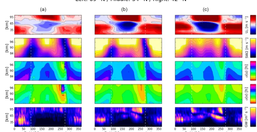
Figure 3 shows composites for similar geographic coor-dinates than Andenes, Juliusruh and Tavistock, of the sim-ulated mean zonal (U0) and meridional (V0) winds, the

Figure 3. HAMMONIA composites of the simulated mean zonal (U0) and meridional winds (V0), migrating semidiurnal (SW2),

non-migrating westward-propagating wave number 1 semidiurnal (SW1), and total semidiurnal (S2) solar tides, and SW2+SW1, over (columna) Andenes, (columnb) Juliusruh and (columnc) Tavistock. The vertical white dashed lines indicate DoYs 90 and 275.

during winter at middle latitudes, where the simulated mean zonal winds are mainly westward. On the other hand, win-tertime mean zonal winds are eastward at high latitudes, in agreement with the observations. The simulated mean merid-ional winds are mainly equatorward during summer below ∼91 km, also in agreement with the observations. However, the poleward winds typically seen in meteor radar measure-ments during winter are not as evident in the simulations, especially at high latitudes. The simulated SW2 tidal com-ponent exhibits similarities with the observed S2 tide: strong amplitudes in winter and both the spring and fall transition times are characterized by a decrease in the activity of SW2, with the decrease seen in the fall being significantly more pronounced and occurring rapidly at all height levels. On the other hand, the amplitudes of SW2 during summer are con-siderably larger than those of the observed S2, while the SW2 fall decrease occurs earlier (∼25 days) and lasts a few more days than in the case of the observed S2. The fall decrease in the simulated total semidiurnal (S2 in Fig. 3) solar tide also takes place∼25 days earlier than in the observations.

The amplitude and seasonal behavior of SW1 are quite different. From Fig. 3, one can clearly see that the ampli-tudes of this tidal component never reach values larger than 20 m s−1and that the lowest values are mainly seen during the summer and the fall. In the spring, SW1 amplitudes over Andenes and Juliusruh remain approximately constant dur-ing the first half of the season, and slightly decrease durdur-ing the second one. Over Tavistock, SW1 exhibits similar am-plitude values throughout most of the spring. During the fall over Andenes and Juliusruh, SW1 amplitudes start decreas-ing around 1 week later than SW2, and they reach the

low-est values approximately one month after SW2 does. Over Tavistock, SW1 exhibits extremely low amplitudes the entire summer and fall. The rest of the semidiurnal tidal compo-nents extracted from HAMMONIA outputs have very small to negligible amplitudes and are not shown here. The sea-sonal behavior of S2 and SW2+SW1 is exactly the same (Fig. 3). The largest differences in amplitude are of only a few m s−1, mainly during summer and early fall. Moreover, the amplitude and seasonal behavior of S2 are very similar to those of SW2, especially during the fall, which suggests that the behavior of the total semidiurnal tide is mainly driven by SW2.

Given that one of the sources of non-migrating tides is the non-linear interaction between migrating tides and station-ary planetstation-ary waves (e.g., He et al., 2017), we also analyzed the PWs extracted from HAMMONIA outputs. However, we found very low to negligible PW activity during equinox times and no significant differences between the spring and fall transition times over all the locations considered in this study. Substantial PW activity was detected in the model only during winter.

3 Discussion

1004 J. F. Conte et al.: Semidiurnal solar tide variability

Figure 4.Composites of the semidiurnal solar tide (S2) and its phase in the zonal and meridional components, over (columna) Andenes, (columnb) Juliusruh and (columnc) Tavistock. The vertical white dashed lines indicate DoYs 90 and 275.

one month earlier in the simulations), as well as in the tidal amplitudes during the spring, the features that characterize the tidal behavior during equinox times are similar in obser-vations and simulations. Further, previous studies have al-ready shown good agreement between observed tides and those simulated by HAMMONIA (e.g., Yuan et al., 2008). Therefore, we assume that one can use the analysis of the simulated tides to explain the behavior of S2 in the observa-tions.

Although both equinox time periods are characterized by a reduction in the activity of the S2 tide, the decrease ob-served in the fall is abrupt, more pronounced and it happens at all height levels at approximately the same time (Fig. 1). Furthermore, despite year-to-year changes in its duration and time of occurrence, the S2 fall decrease repeats every single year at both middle and high latitudes (Fig. 2). Laskar et al. (2016) suggested that a possible explanation of this feature may be that distinct migrating and non-migrating compo-nents of S2 behave differently during these periods. After ex-tracting the tides from HAMMONIA simulations, we found that the simulated S2 tide is primarily determined by SW2 and SW1, which happen to present distinct behaviors during the spring and fall transition times. From Fig. 3, it can be seen that during the spring, SW2 decreases but SW1 maintains similar amplitude values or slightly decreases. During the fall, both tides decrease, although SW1 does it later. One can thus postulate that since SW1 does not decrease significantly during the spring, this allows the S2 tide to maintain larger amplitudes than those observed during the fall. On the other hand, it seems that the influence of SW1 in the fall is not as relevant, given that this tidal component decreases later than

SW2, but S2 decreases at the same time and with the same intensity as SW2. In other words, the observed S2 tide creases during both equinox time periods because SW2 de-creases, but during the spring the reduction of S2 is not as pronounced due to sustained higher amplitudes of SW1. In the fall, the observed decrease in S2 is more pronounced due to a more intense and longer decrease in SW2.

Tavi-Figure 5.HAMMONIA composites of the simulated mean zonal (U0) wind, the migrating semidiurnal solar (SW2) tide, SW2 phases in

the zonal (φ (u)) and meridional (φ (v)) components, and gravity wave kinetic energy over (columna) Andenes, (columnb) Juliusruh and (columnc) Tavistock. The vertical white dashed lines indicate DoYs 90 and 275. Notice the different height range in the case ofU0and the

GWs.

stock. The latter were obtained in the same way as for the observations.

Atmospheric tides are strongly influenced by mean winds and other types of waves (e.g., McLandress, 2002). Particu-larly, gravity waves propagating up from the troposphere can-not reach higher altitudes than those where their phase veloc-ities match the wind velocity (e.g., Holton, 1983). However, during the fall transition time, the zonal wind in the strato-sphere and mesostrato-sphere reverses from westward to eastward (see Fig. 5). Espy and Stegman (2002) showed that this re-versal of the wind allows GWs to freely propagate upwards and reach the MLT region. Therefore, it is possible that the change seen in the phase of S2 is the result of interactions be-tween this tide and GWs (e.g., Fritts and Vincent, 1987). By comparing Figs. 1 and 4, one can see that the enhancement of the gravity wave activity detected during the fall occurs at approximately the same time the phase of S2 shifts signif-icantly. In the case of HAMMONIA simulations, the grav-ity wave activgrav-ity also enhances considerably during the fall (Fig. 5). Andenes does not show such a strong enhancement, although it is clear that there is more GW activity during the fall than in the spring. GWs may naturally result from model simulations (e.g., Shepherd et al., 2000), but they strongly depend on the resolution of the model. As mentioned before, HAMMONIA runs at T31, which means that the smallest waves resolved by the model will have a length of more than 1000 km. This clearly imposes limitations to our analysis, since the gravity waves extracted from HAMMONIA simu-lations will only represent a small part of the actual GW spec-trum and different parts of the latter may interact differently

with S2. On the other hand, given that parameterized gravity waves can act only where they break (e.g., Sarin et al., 1996), a thorough analysis of the mean flow is necessary in order to assess their impact on the tidal behavior. This is clearly out of the scope of the present study. Nonetheless, if one takes into consideration that the results based on the simulated grav-ity waves are only applicable to long-scale waves, it follows that observations and model simulations reveal that the long-wave GW activity enhances at approximately the same time the semidiurnal solar tide exhibits a strong shift in its phase and a pronounced decrease in its amplitude. Consequently, one may speculate that the change seen during the fall in the phase of the S2 tide, as well as the decrease in its ampli-tude, are partly due to interactions between SW2 and gravity waves. Future efforts will be focused on direct comparisons of the observed SW2 with GWs, as well as with planetary waves. For that, we plan to use multiple radars to separate SW2 and SW1 from the actual measurements, by means of a phase differencing technique (He et al., 2018).

1006 J. F. Conte et al.: Semidiurnal solar tide variability

spring, the ozone levels are slightly reduced during the fall. However, this difference is not large enough so as to attribute the sudden decrease in S2 to a depletion of ozone.

4 Conclusions

Based on comparisons of meteor radar measurements with HAMMONIA model simulations, we showed that the differ-ences exhibited by the semidiurnal solar tide (S2) observed at middle and high latitudes of the Northern Hemisphere be-tween equinox times are mainly due to distinct behaviors of the migrating semidiurnal (SW2) and the non-migrating westward-propagating wave number 1 semidiurnal (SW1) tidal components. Specifically, during the fall both SW2 and SW1 decrease, while during the springtime SW2 decreases but SW1 remains approximately constant or decreases only slightly. The decrease shown by SW1 during the fall occurs later than that of SW2 and S2, which indicates that the be-havior of S2 is mainly driven by the migrating component. Nonetheless, the influence of SW1 is necessary to explain the behavior of S2 during the spring. Contributions by other semidiurnal tidal components were found to be very small to negligible.

In addition, we have shown that during the fall transi-tion, at approximately the same time the observed S2 tide decreases, a downward propagated phase shift (of ∼2 h or more) can be seen in both horizontal components of this tide. The same feature was found in the model simulations, but in both horizontal components of SW2. Furthermore, our me-teor radar observations show an increase in the gravity wave activity during this time interval, possibly indicating that the phase shift, and the decrease in the amplitude of the semid-iurnal solar tide, may be partly due to interactions between SW2 and gravity waves.

Data availability. The Andenes and Juliusruh meteor radar data are available upon request from Gunter Stober. To obtain access to Tavi-stock meteor radar data and/or HAMMONIA model simulations, please contact Peter Brown and/or Hauke Schmidt.

Competing interests. The authors declare that they have no conflict of interest.

Special issue statement. This article is part of the special issue “Dynamics and interaction of processes in the Earth and its space environment: the perspective from low Earth orbiting satellites and beyond”. It is not associated with a conference.

Acknowledgements. This work was supported by the Deutsche Forschungsgemeinschaft (DFG, German Research Foundation) un-der SPP 1788 (DynamicEarth) project CH 1482/1-1 (DYNAMITE).

The authors would like to thank Nick Pedatella from NCAR and the members of the Tides matrix group at IAP for the fruitful dis-cussions that helped to improve the quality of this work.

The topical editor, Claudia Stolle, thanks two anonymous refer-ees for help in evaluating this paper.

References

Angelats i Coll, M. and Forbes, J. M.: Nonlinear interactions in the upper atmosphere: Thes=1 ands=3 nonmigrating semid-iurnal tides, J. Geophys. Res.-Space, 107, SIA 3-1–SIA 3-15, https://doi.org/10.1029/2001JA900179, 2002.

Chapman, S. and Lindzen, R. S.: Atmospheric Tides, 200 pp., D. Reidel Publishing Co., Springer, the Netherlands, 1970. Charlton, A. J. and Polvani, L. M.: A New look at stratospheric

sud-den warmings, Part I: Climatology and modeling Benchmarks, J. Climate, 20, 470–488, https://doi.org/10.1175/JCLI3994.1, 2007.

Chau, J. L., Hoffmann, P., Pedatella, N. M., Matthias, V., and Stober, G.: Upper mesospheric lunar tides over middle and high latitudes during sudden stratospheric warming events, J. Geophys. Res.-Space, 120, 3084–3096, https://doi.org/10.1002/2015JA020998, 2015.

Eckermann, S. D. and Marks, C. J.: An idealized ray model of grav-ity wave-tidal interactions, J. Geophys. Res., 101, 21195–21212, 1996.

Espy, P. J. and Stegman, J.: Trends and variability of mesospheric temperature at high-latitudes, Phys. Chem. Earth, 27, 543–553, https://doi.org/10.1016/S1474-7065(02)00036-0, 2002. Forbes, J. M.: Middle atmosphere tides, J. Atmos. Terr. Phys., 46,

1049–1067, 1984.

Forbes, J. M. and Vial, F.: Monthly simulations of the solar semid-iurnal tide in the mesosphere and lower thermosphere, J. At-mos. Terr. Phys., 51, 649–661, https://doi.org/10.1016/0021-9169(89)90063-9, 1989.

Fritts, D. C. and Alexander, M. J.: Gravity wave dynamics and effects in the middle atmosphere, Rev. Geophys., 41, 1003, https://doi.org/10.1029/2001RG000106, 2003.

Fritts, D. C. and Vincent, R. A.: Mesospheric momentum flux stud-ies at Adelaide, Australia: Observations and a gravity wave-tidal interaction model, J. Atmos. Sci., 44, 605–619, 1987.

Fuller-Rowell, T., Wu, F., Akmaev, R., Fang, T.-W., and Araujo-Pradere, E.: A whole atmosphere model simulation of the im-pact of a sudden stratospheric warming on thermosphere dynam-ics and electrodynamdynam-ics, J. Geophys. Res.-Space, 115, A00G08, https://doi.org/10.1029/2010JA015524, 2010.

Giorgetta, M. A., Manzini, E., Roeckner, E., Esch, M., and Bengts-son, L.: Climatology and forcing of the quasi-biennial oscillation in the MAECHAM5 model, J. Climate, 19, 3882–3901, 2006. Hagan, M. E. and Forbes, J. M.: Migrating and nonmigrating

diur-nal tides in the middle and upper atmosphere excited by tropo-spheric latent heat release, J. Geophys. Res., 107, ACL 6-1–ACL 6-15, https://doi.org/10.1029/2001JD001236, 2002.

He, M., Chau, J. L., Stober, G., Hall, C. M., Tsutsumi, M., and Hoffmann, P.: Application of Manley–Rowe relation in analyzing nonlinear interactions between planetary waves and the solar semidiurnal tide during 2009 sudden stratospheric warming event, J. Geophys. Res.-Space, 122, 10783–10795, https://doi.org/10.1002/2017JA024630, 2017.

He, M., Chau, J. L., Stober, G., Li, G., Ning, B., and Hoffmann, P.: Relations between semidiurnal tidal variants through diagnos-ing the zonal wavenumber usdiagnos-ing a phase differencdiagnos-ing technique based on two ground-based detectors, J. Geophys. Res.-Atmos., 123, 4015–4026, https://doi.org/10.1002/2018JD028400, 2018. Hines, C. O.: Doppler-spread parameterization of gravity wave

mo-mentum deposition in the middle atmosphere. Part 2: Broad and quasi monochromatic spectra, and implementation, J. Atmos. Sol.-Terr. Phy., 59, 387–400, 1997a.

Hines, C. O.: Doppler-spread parameterization of gravity wave mo-mentum deposition in the middle atmosphere. Part 1: Basic for-mulation, J. Atmos. Sol.-Terr. Phy., 59, 371–386, 1997b. Hocking, W., Fuller, B., and Vandepeer, B.: Real-time

deter-mination of meteor-related parameters utilizing modern dig-ital technology, J. Atmos. Sol.-Terr. Phy., 63, 155–169, https://doi.org/10.1016/S1364-6826(00)00138-3, 2001. Hocking, W. K. and Thayaparan, T.: Simultaneous and collocated

observations of winds and tides by MF and meteor radars over London, Canada (43◦N, 81◦W), during 1994–1996, Radio Sci., 32, 833–865, 1997.

Hoffmann, P., Singer, W., Keuer, D., Hocking, W. K., Kunze, M., and Murayama, Y.: Latitudinal and longitudinal variabil-ity of mesospheric winds and temperatures during stratospheric warming events, J. Atmos. Sol.-Terr. Phy., 69, 2355–2366, https://doi.org/10.1016/j.jastp.2007.06.010, 2007.

Hoffmann, P., Becker, E., Singer, W., and Placke, M.: Sea-sonal variation of mesospheric waves at northern middle and high latitudes, J. Atmos. Sol.-Terr. Phy., 72, 1068–1079, https://doi.org/10.1016/j.jastp.2010.07.002, 2010.

Holton, J. R.: The Influence of Gravity Wave Breaking on the General Circulation of the Middle Atmosphere, J. Atmos. Sci., 40, 2497–2507, https://doi.org/10.1175/1520-0469(1983)040<2497:TIOGWB>2.0.CO;2, 1983.

Jacobi, C., Portnyagin, Y. I., Solovjova, T. V., Hoffmann, P., Singer, W., Fahrutdinova, A. N., Ishmuratov, R. A., Beard, A. G., Mitchell, N. J., Muller, H. G., Schminder, R., Kürschner, D., Manson, A. H., and Meek, C. E.: Climatology of the semid-iurnal tide at 52–56◦N from ground-based radar wind mea-surements 1985–1995, J. Atmos. Sol.-Terr. Phy., 61, 975–991, https://doi.org/10.1016/S1364-6826(99)00065-6, 1999. Kinnison, D. E., Brasseur, G. P., Walters, S., Garcia, R. R., Marsh,

D. R., Sassi, F., Harvey, V. L., Randall, C. E., Emmons, L., Lamarque, J. F., Hess, P., Orlando, J. J., Tie, X. X., Ran-del, W., Pan, L. L., Gettelman, A., Granier, C., Diehl, T., Niemeier, U., and Simmons, A. J.: Sensitivity of chemical trac-ers to meteorological paramettrac-ers in the MOZART-3 chemi-cal transport model, J. Geophys. Res.-Atmos., 112, D20302, https://doi.org/10.1029/2006JD007879, 2007.

Laskar, F. I., Chau, J. L., Stober, G., Hoffmann, P., Hall, C. M., and Tsutsumi, M.: Quasi-biennial oscillation modulation of the middle- and high-latitude mesospheric semidiurnal tides during August–September, J. Geophys. Res.-Space, 121, 4869–4879, https://doi.org/10.1002/2015JA022065, 2016.

Lott, F. and Miller, M. J.: A new subgrid-scale orographic drag pa-rameterization: Its formulation and testing, Q. J. Roy. Meteor. Soc., 123, 101–127, 1997.

Manson, A., Meek, C., Hagan, M., Hall, C., Hocking, W., Mac-Dougall, J., Franke, S., Riggin, D., Fritts, D., Vincent, R., and Burrage, M.: Seasonal variations of the semi-diurnal and diurnal tides in the MLT: Multi year MF radar observations from 2 to 70◦N, and the GSWM tidal model, J. Atmos. Sol.-Terr. Phy., 61, 809–828, 1999.

Manzini, E., Giorgetta, M. A., Esch, M., Kornblueh, L., and Roeckner, E.: The influence of sea surface temperatures on the Northern winter stratosphere: Ensemble simulations with the MAECHAM5 model, J. Climate, 19, 3863–3881, 2006. Matthias, V., Shepherd, T. G., Hoffmann, P., and Rapp, M.: The

Hiccup: a dynamical coupling process during the autumn tran-sition in the Northern Hemisphere – similarities and differences to sudden stratospheric warmings, Ann. Geophys., 33, 199–206, https://doi.org/10.5194/angeo-33-199-2015, 2015.

McCormack, J., Hoppel, K., Kuhl, D., de Wit, R., Stober, G., Espy, P., Baker, N., Brown, P., Fritts, D., Jacobi, C., Janches, D., Mitchell, N., Ruston, B., Swadley, S., Viner, K., Whit-comb, T., and Hibbins, R.: Comparison of mesospheric winds from a high-altitude meteorological analysis system and me-teor radar observations during the boreal winters of 2009/2010 and 2012/2013, J. Atmos. Sol.-Terr. Phy., 154, 132–166, https://doi.org/10.1016/j.jastp.2016.12.007, 2016.

McLandress, C.: The seasonal variation of the propagating diurnal tide in the mesosphere and lower thermosphere. Part I: The role of gravity waves and planetary waves, J. Atmos. Sci., 59, 893–906, https://doi.org/10.1175/1520-0469(2002)059<0893:TSVOTP>2.0.CO;2, 2002.

Pancheva, D., Mukhtarov, P., and Andonov, B.: Global structure, seasonal and interannual variability of the migrating semidiur-nal tide seen in the SABER/TIMED temperatures (2002–2007), Ann. Geophys., 27, 687–703, https://doi.org/10.5194/angeo-27-687-2009, 2009.

Riggin, D., Meyer, C., Fritts, D., Jarvis, M., Murayama, Y., Singer, W., Vincent, R., and Murphy, D.: MF radar observations of sea-sonal variability of semidiurnal motions in the mesosphere at high northern and southern latitudes, J. Atmos. Sol.-Terr. Phy., 65, 483–493, 2003.

Rossby, C.-G.: Relation between variations in the intensity of the zonal circulation of the atmosphere and the displacements of the semipermanent centers of action, J. Mar. Res., 2, 38–55, 1939. Sarin, V. B., Forichon, M., and Le Treut, H.: Parameterization and

influence of the orographic gravity-wave drag in the LMD-GCM, Math. Comput. Model., 24, 71–84, https://doi.org/10.1016/0895-7177(96)00108-2, 1996.

Schmidt, H., Brasseur, G. P., Charron, M., Manzini, E., Gior-getta, M. A., Diehl, T., Fomichev, V. I., Kinnison, D., Marsh, D., and Walters, S.: The HAMMONIA Chemistry Climate Model: Sensitivity of the Mesopause Region to the 11-year Solar Cycle and CO₂ Doubling, J. Climate, 19, 3903–3931, https://doi.org/10.1175/JCLI3829.1, 2006.

1008 J. F. Conte et al.: Semidiurnal solar tide variability

Shepherd, T. G., Koshyk, J. N., and Ngan, K.: On the nature of large-scale mixing in the stratosphere and mesosphere, J. Geophys. Res., 105, 12433–12446, https://doi.org/10.1029/2000JD900133, 2000.

Smith, A. K.: Global Dynamics of the MLT, Surv. Geophys., 33, 1177–1230, 2012.

Stober, G., Matthias, V., Jacobi, C., Wilhelm, S., Höffner, J., and Chau, J. L.: Exceptionally strong summer-like zonal wind rever-sal in the upper mesosphere during winter 2015/16, Ann. Geo-phys., 35, 711–720, https://doi.org/10.5194/angeo-35-711-2017, 2017.

Taylor, M. J., Pendleton, W. R., Liu, H.-L., She, C. Y., Gardner, L. C., Roble, R. G., and Vasoli, V.: Large amplitude perturba-tions in mesospheric OH Meinel and 87-Km Na lidar temper-atures around the autumnal equinox, Geophys. Res. Lett., 28, 1899–1902, https://doi.org/10.1029/2000GL012682, 2001.

Yi˘git, E. and Medvedev, A. S.: Influence of parameterized small-scale gravity waves on the migrating diurnal tide in Earth’s thermosphere, J. Geophys. Res.-Space, 122, 4846–4864, https://doi.org/10.1002/2017JA024089, 2017.