The Impact of Bias Correction and Model Selection on Passing Temperature Thresholds

(1)

White Rose Research Online URL for this paper:

http://eprints.whiterose.ac.uk/150379/

Version: Published Version

Article:

Gohar, LK, Lowe, JA orcid.org/0000-0002-8201-3926 and Bernie, D (2017) The Impact of

Bias Correction and Model Selection on Passing Temperature Thresholds. Journal of

Geophysical Research: Atmospheres, 122 (22). 12,045-12,061. ISSN 2169-897X

https://doi.org/10.1002/2017JD026797

[email protected]

https://eprints.whiterose.ac.uk/

Reuse

Items deposited in White Rose Research Online are protected by copyright, with all rights reserved unless

indicated otherwise. They may be downloaded and/or printed for private study, or other acts as permitted by

national copyright laws. The publisher or other rights holders may allow further reproduction and re-use of

the full text version. This is indicated by the licence information on the White Rose Research Online record

for the item.

Takedown

If you consider content in White Rose Research Online to be in breach of UK law, please notify us by

(2)

The Impact of Bias Correction and Model Selection

on Passing Temperature Thresholds

L. K. Gohar1 , J. A. Lowe1,2, and D. Bernie1 1_{Met Of}

ﬁce, Exeter, UK,2Priestley International Centre for Climate, University of Leeds, Leeds, UK

Abstract

Knowledge of when specific global or local temperature levels are reached is important for decision makers in that it provides a time frame over which adaptation strategies for temperature-related climate impacts need to be put in place. The time frame varies depending on the adaptation strategy but can range from a few years to the order of decades. Climate models, however, show a high degree of uncertainty in the timing of passing specific warming levels, limiting their use in adaptation policy development. This study examines the impact of two approaches, which may reduce the uncertainty in modeled timing of reaching specific warming levels. First, the use of different performance metrics to preferentially weight model ensembles and second, the application of four bias correction approaches. Using the Coupled Model Intercomparison Project phase 5 simulations of the Representative Concentration Pathways, our results show that both selecting models based on performance and bias correcting model data reduce the spread in timing of specific warming levels reached in thefirst half of the century by up to 50% in some regions. This implies the potential of these approaches to support adaptation planning.

1. Introduction

The United Nations Framework Convention on Climate Change aims to limit global annual mean tempera-ture rise to well below 2°C above preindustrial levels (United Nations/Framework Convention on Climate Change, 2015) based on a large body of research into what constitutes dangerous anthropogenic interfer-ence in the climate system. Research over the recent years has focused mainly on the uncertainty in the magnitude of the temperature threshold that would result in undesirable impacts (Field et al., 2014; Solomon et al., 2007; Stocker et al., 2014). In this study we shift the focus from uncertainty in the magnitude of temperature rise in a given year, to the timing of when a temperature threshold is passed. Knowing when temperature thresholds are crossed is important because climate impacts occur at different temperatures. For example, the sensitivity of crop to temperatures (Porter et al., 2014) differs to the impact of heat stress thresholds on labor productivity (Dunne et al., 2013). There are also different timescales involved in the realization of climate impacts which, together with knowledge of when a threshold may be exceeded, are important for adaptation responses. For example, in the short term, changes in crop-related impacts might involve planting earlier/later while long-term adaptation might consider new farming systems (Oleson et al., 2011). A better understanding of the timing of any given temperature threshold and the associated negative consequences would enable more effective and resilient adaptation strategies to be developed.

Past studies show a range of values of when particular temperature thresholds might be exceeded on both the global and regional levels. Global annual mean values yield estimates of passing 2°C ranging from the 2040s to the 2060s for multimodel mean simulations of high emissions scenarios when considering decadal to 20 year means (Collins et al., 2013; Joshi et al., 2011; Meehl et al., 2007). The best estimates of when 4°C will be passed under high emissions scenarios range from the 2070s to 2090s (Adams et al., 2013; Betts et al., 2011; Collins et al., 2013). Individual models project higher temperatures by the end of this century for high emissions scenarios (Collins et al., 2013). However, in this work we focus on multimodel ensemble timings to better capture the uncertainty in our understanding of the climate response to high forcing scenarios. These estimates of the timings vary by up to 30 years with the uncertainty partly arising from our incomplete under-standing of the climate’_{s responses to greenhouse gas (GHG) emissions. Another source of uncertainty in} future warming levels is the speciﬁcation of future emissions of GHG which depend on the interconnected socioeconomic technical as well as political development. Other sources of uncertainty include the structural uncertainty related to the modeling of the climate (Hawkins & Sutton, 2009). Attempts to account for these sources of uncertainty have been made through the use of multimodel ensembles, perturbed parameter ensembles, and a range of future radiative forcing pathways. Other factors that may also inﬂuence the

Journal of Geophysical Research: Atmospheres

RESEARCH ARTICLE

10.1002/2017JD026797

Key Points:

•_{Selecting models on the basis of} performance metrics can reduce the spread in the timings of passing warming thresholds by up to 50% •_{Applying a bias correction technique}

to climate simulations can reduce the spread in the timings of passing grid box-scale warming thresholds by up to 50%

•The narrowing of the spread in timings for warming thresholds at the grid box scale has the potential to affect the time frame adopted for effective adaptation strategies

Supporting Information:

•_{Supporting Information S1}

Correspondence to:

L. K. Gohar,

laila.gohar@metofﬁce.gov.uk

Citation:

Gohar, L. K., Lowe, J. A., & Bernie, D. (2017). The impact of bias correction and model selection on passing tem-perature thresholds.Journal of Geophysical Research: Atmospheres,122, 12,045–_{12,061. https://doi.org/10.1002/} 2017JD026797

Received 15 MAR 2017 Accepted 26 OCT 2017

Accepted article online 3 NOV 2017 Published online 16 NOV 2017

(3)

uncertainty are the definition of passing a temperature threshold, which includes some degree of temporal averaging (typically over decades), and the specification of a baseline from which the change is calculated. Both of these can introduce some uncertainty although to a lesser extent than from the specification of future GHG emissions pathways and the uncertainty in climate response (Hawkins et al., 2017; Hawkins & Sutton, 2016). The length of the averaging period is important as it reduces the impact of natural variability on warm-ing trends; this is discussed in the followwarm-ing section where we define the passing of a specific warming level. Hawkins and Sutton (2016) show that changing the reference period influences the present-day warming relative to observations. This change in relative warming is in both magnitude and in the estimated range, as the state of the climate during the reference period might be unlike adjacent periods, for example, if a reference period is chosen during a period of volcanic activity which temporarily depressed global tempera-tures relative to the several decades either side.

This study explores climate change projections from the World Climate Research Programme Coupled Model Intercomparison Project phase 5 (CMIP5) multimodel data set (Taylor et al., 2012) to assess the impact of model bias on the estimated timing of passing speciﬁc warming levels (SWLs). The bias explored here is sepa-rated into two types. First, the bias is introduced by subselecting based on performance rather than including all models in an ensemble. The motivation behind this is to explore the impact of choosing a“_better”_{set of} models to comprise a multimodel ensemble and then to assess how this would affect the timings of passing SWLs. The second aspect of bias examined is the impact of bias correction techniques used to reconcile differences between model simulations of the present day and observations, an approach common in impact studies. The motivation of examining this aspect of bias is to assess how bias correction techniques inﬂuence the timings of passing SWLs and to understand how information on future climate changes in simulations are affected by the process of different bias correction approaches. A novel aspect of this work is that it assesses the impact of model selection and applying bias corrections to model simulations on the timings of crossing temperature thresholds and the associated uncertainty, both globally and regionally (i.e., at the grid box level). We believe that this has not been looked at in detail before and is relevant to research into future impact assessments and associated adaptation planning.

Interpreting the uncertainty described by a climate model ensemble depends on the ensemble design, the model independence (considered here in terms of shared formulation), and whether the models have been evaluated (Knutti, 2010). The CMIP5 multimodel ensemble is an“_{ensemble of opportunity}”_{as it does not} sample model uncertainties systematically nor randomly (Tebaldi & Knutti, 2007). Each model has been indi-vidually evaluated to some extent, but a common approach is to include all models and assume that they are all equally likely in lieu of a robust assessment of which models are better than others (Knutti, 2010). This approach was adopted in the Intergovernmental Panel on Climate Change’_s_ﬁ_{fth assessment report (IPCC} AR5) and all previous CMIPs. Performance-based metrics have, however, been developed to benchmark climate models against observations of particular set of metrics. These metrics provide a measure of conﬁ -dence in model skill, but designing multivariate metrics is a relatively new area of research. While there is some diversity in the literature, relatively few performance metrics exist (Barker & Taylor, 2016; Gleckler et al., 2008; Reichler & Kim, 2008; Watterson et al., 2014). Constraining models based on how well they simu-late observations implies model skill for present day. But this does not necessarily imply skill for future climate change projections (Knutti, 2010; Raisanen et al., 2010; Reifen & Toumi, 2009; Sanderson & Knutti, 2012) unless there is a clear physical relationship between observables and the projections, for example, the decline in Arctic sea ice (Boe et al., 2009). Furthermore, knowing that models have varying skill in simulating present-day observations (Gleckler et al., 2008; Reichler & Kim, 2008) and that there is model interdependence (Masson & Knutti, 2011) makes the assumption of all models being equally likely harder to justify (Sanderson et al., 2015).

(4)

from observations in a chosen baseline period (Haerter et al., 2011; Hempel et al., 2013; Piani et al., 2010). The main assumptions in bias correction methods are that the quality of the observations determines the quality of the bias correction, that the bias behavior is time invariant (stationarity), and that the methods cannot cor-rect for fundamentally misrepresented physical processes (Ehret et al., 2012). The time invariant assumption has been criticized, as there is evidence of nonstationarity in the climate response to a warming world such as in extreme precipitation and evapotranspiration (Milly et al., 2008). Li et al., (2010) show a dependence on the baseline period used to correct the model simulations against observations. In this study, we explore the implications of applying four different bias correction techniques for the timing of passing SWL at global and grid box (approximately 100 km) scales.

Theﬁrst part of the analysis assesses the impact on timings of passing SWLs, globally and at the grid box scale, of subselecting models from the CMIP5 ensemble based on different performance metrics. The second part of the analysis studies the implications of various bias correction methods on the timings of passing SWL.

2. Materials and Methods

2.1. Climate Model Simulations

The climate model simulations used in this work were drawn from the CMIP5 multimodel data set used exten-sively in IPCC AR5. Simulations from 38 CMIP5 models are used to look at the timings of passing SWL of 2°C and 4°C based on future forcing scenarios described by the Representative Concentration Pathways (RCPs, Moss et al., 2010). The highest forcing pathway, RCP8.5 (Riahi et al., 2007), was chosen as it is the only RCP to provide useful information on passing of 4°C. Conversely, a mitigation pathway, RCP4.5 (Clarke et al., 2007; Smith & Wigley, 2006; Wise et al., 2009), is used to provide another pathway (in addition to RCP8.5) passing 2°C. This was chosen as the second pathway as the lowest forcing RCP (RCP2.6) had fewer simulations reaching 2°C, and RCP6.0 had fewer model simulations available to examine owing to its delayed release during the CMIP5 process.

The data are available as spatially resolved monthly means on the native models grids and were regridded on to a N96 grid for the purpose of comparison and aggregation. The regridding is aﬁrst-order, conservative interpolation. The regridded data were aggregated spatially and temporally to calculate the global annual mean near surface warming. Analysis is presented in sections 4.1.1 and 4.2.1. A similar aggregation was done for the seasonal analysis for June/July/August and December/January/February, but as results were similar to those for annual means the analysis of seasonal data is provided as supporting information. Analysis of passing SWL at the grid box level is based on the spatially resolved monthly mean data with analysis in sections 4.1.2 and 4.2.2.

The number of models in the CMIP5 ensemble used in the bias correction (36 models) analysis differs from the previous performance metrics analysis (38 models), due to the data availability on the required time reso-lution for the bias correction techniques. Hence, there will be differences in the raw cumulative frequencies (CFs) and global maps of the timings of passing temperature thresholds. These models are listed in Table S1 in the supporting information.

2.2. Data and Assumptions Used for the Bias-Corrected Simulations

The baseline period chosen to perform the bias corrections is the 1986–_{2005 period, and the ERA-interim} data (Dee et al., 2011) are used as a proxy for the observations because the spatial coverage over the globe is complete and gridded. The ERA-interim data were regridded to a N96 grid following the same method as for the CMIP5 simulations.

(5)

correction techniques more difﬁcult to isolate. Therefore, pattern scaling was used on the multimodel mean warming from preindustrial to the baseline period and scaled so that the global annual mean warming matched the observed estimate of 0.61°C. This ensures that the warming from preindustrial to the 1986–_{2005 mean period is the same in all models, and the differences in our analysis arise only from the bias} correction techniques considered. Recent work by Hawkins et al. (2017) have found some sensitivity of warming estimates to the choice of preindustrial time period, but extension of their study to the timing of warming levels is beyond the scope of the present study.

Finally, in order to limit the noise of the results, only grid points where more than six models indicate a passing of the warming threshold are considered in allﬁgures.

2.3. The Selection Criteria: Performance Metrics

We use three performance metrics. Theﬁrst is a global metric from Watterson et al., (2014) which adopts a method, similar to that of Reichler and Kim (2008), of a single metric based on the average of the nondimen-sional Mielke measure (root-mean-square error) for three climate impact-related parameters (the 2 m temperature, precipitation, and the mean sea level pressure). These are time averaged over the present day (and over the seasons). This metric has been used as a measure of model performance (Meehl et al., 2007). However, the metric is still inﬂuenced by statistical uncertainty in the model and observations. In order to subselect the better models, simulations were ranked based on the global mean performance (see Table 1 in Watterson et al., 2014) and the top half selected as better.

The second metric is an update of Gleckler et al. (2008) for the CMIP5 models (Flato et al., 2013). There are several individual root-mean-square error metrics presented in this second set of metrics (e.g., near-surface temperature, zonal and meridional winds, top of the atmosphere radiationﬁelds, and precipitation), and without evidence to support particular metrics being better predictors of overall model performance we retain all the metrics examined. The subselection for this metric was based on models which had a minimum number of variables (four in this study) performing better than the median CMIP5 error.

Thefinal metric used in this study is from the recently published work by Barker and Taylor (2016), which bases the metrics on variables relevant to the Earth’_{s energy budget. The selection criteria for this metric were} based on the topfive performing metrics compared to the ensemble mean metric. Those models that performed well in allfive of these metrics were chosen.

The list of models included in the CMIP5 ensemble and the models selected by the three different perfor-mance metrics are given in Table S1. While some models appear more often as better models in Table S1, this should not be taken to imply that the performance of other models is poor rather that they do not perform as well against the speciﬁc metrics examined here.

2.4. Bias Correction Techniques

There are a growing number of methods for correcting climate model biases. The four examined in this study illustrate how the corrections can be applied to the modeled mean, variance, and higher moments of a distribution (see Teutschbein & Seibert, 2012; Themeßl et al., 2011 and Watanabe et al., 2012 for more detailed overviews).

Theﬁrst bias correction technique (BC1) is the simplest. This type of linear scaling involves adjusting the modeled future data relative to a baseline period. The observed change from the baseline period is then added to the adjusted modeled data. The aim of this simple method is to match the modeled meanﬁeld in the baseline period to observations.

XLSð Þ ¼t Obase XbaseþXfutð Þt (1)

(6)

The second bias correction technique (BC2) is a type of variance scaling and is often referred to as the change factor method (Hawkins et al., 2013). This is a popular bias correction technique used in impact modeling due to its simplicity (e.g., estimating river runoff in Arnell et al., 2003, Prudhomme et al., 2014). The variance scal-ing adjusts both the modeled mean and the variance but uses the observed variability and adds the model anomalies on to it:

XVSð Þ ¼t Xfutþ

σXfut

σXbase

·Obaseð Þt Xbase

(2)

The sigmas are the standard deviations of the observations or simulations over the baseline period.

A simple quantile mapping technique is the third type of bias correction (BC3). In quantile mapping, the empirical cumulative distribution probabilities are estimated using a table of empirical percentiles. Linear interpolation is used to estimate values in between the percentiles. If the modeled values lie outside the range of observations, the highest quantiles in the observational period are used (Themeßl et al., 2012). This type of bias correction technique considers the entire distribution of theﬁeld in the baseline period and is more suitable when considering changes in the extreme values, for example, in impacts related to hydrological processes.

XQMð Þ ¼t FO 1ðFXðXfutð ÞtÞÞ (3)

whereFrepresents the cumulative distribution function, which maps the modeled data to observations.

The Inter-Sectoral Impact Model Intercomparison Project (ISIMIP) quantile mapping technique (Hempel et al., 2013) is the fourth type of bias correction considered in this study (BC4). This is a trend-preserving quantile mapping method and was used in the ISIMIP project to look at various sector-speciﬁc climate change impacts such asﬂooding (Schleussner et al., 2016) and impact on crop yields (Zhao et al., 2016). The method consists of separating the timescales involved in the data and applying corrections on each timescale (e.g., monthly and daily timescales to correct the monthly mean simulations). A basic corrective addition is applied to the longest timescale which corrects the mean change seen in the modeled data using observations, thereby preserving the“_trend.”_{Hence, it is very similar to the linear scaling method on the annual mean timescale.} The variability is corrected on the smaller timescales by adjusting the residuals from the mean using a quan-tile mapping transfer function based on the observed and modeled data during the baseline period. In this work, residuals calculated on the monthly timescale are corrected using the quantile mapping technique.

X_BC_{ð Þ ¼}t C_þX_fut_{ð Þ þ}t _ΔXe_fut_{ð Þ}t _(4a)

C_¼Obase Xbase (4b)

ΔXefutð Þ ¼t B·ΔXfutð Þt (4c)

whereCis the constant from the largest timescale correction factor on the mean and this step of the bias correction preserves the trend seen in the modeled data. The correction on the residual step (equation (4c)) performs a quantile mapping on the anomaly from the mean using a parametric transfer function constructed from the cumulative distribution functions of the observations and the modeled data over the baseline period to derive the slope of the curve B.

3. De

ﬁ

ning Crossing a Speci

ﬁ

c Warming Threshold

(7)

for SWLs of 2°C or 4°C (not shown). The baseline period from which the SWL is deﬁned in this work is preindustrial unless otherwise stated, and although the choice of the baseline period can affect the timings of passing SWLs (Hawkins et al., 2017), we chose the period 1861–_{1880 for} ease of comparison with past studies of estimates of passing temperature thresholds. In the rest of the paper we will refer to SWLs of 2°C or 4°C as SWL2 and SWL4. In the grid box analysis, we follow the same method for calculating the timings of crossing a SWL at each grid box and for each model. The global maps of the grid box timings are of the mean of timings of exceeding a SWL. Therefore, there are a different number of models timings included in the mean for different grid boxes.

4. Results: The Impact on Timings of When 2°C and 4°C

Are Passed

4.1. Selection Based On Performance Metrics

4.1.1. The Impact of Model Selection on the Global Annual Mean Scale

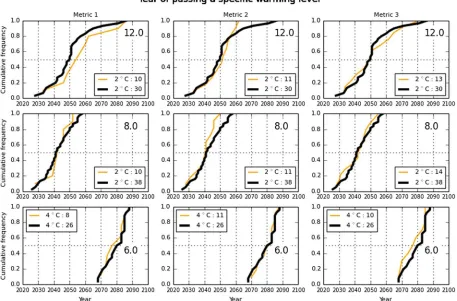
[image:7.612.41.280.90.248.2]

The timings of when the full set of models pass SWL2 for RCP4.5 simulations are shown as a cumulative frequency, CF (Figure 2, top left column). Models pass SWL2 in CMIP5 from the late 2020s to 2085 with a median year of 2050. The application of the performance metrics to RCP4.5 (Figure 2, top row) generally results in a narrowing of the CFs shown. The metric 2 CF range is reduced by 20 years with the latest year Figure 1.The impact of changing the time averaging period for calculating

the speciﬁc warming level (SWL).

[image:7.612.78.535.379.680.2]

(8)

of passing SWL2 being 2061. The CF for metric 3 has a range from the early 2030s to 2080. The median SWL2 year is 4 years later for metric 1 CF, 2 years later for metric 2, and the same as the unselected CF for metric 3. Similar behavior is seen for RCP8.5 CFs but with a few differences; there is a reduction in range across all metrics but not as large as those seen for RCP4.5 (less than 10 years), and the median SWL2 year is earlier in both metrics 1 and 2 CFs but by less than 5 years. The CF for metric 2 shows no change in the median SWL2 year. The metric 1 CF for RCP4.5 consists of later timings of passing SWL2 compared to the full set of models, while there is little change between the CFs for RCP8.5. This suggests that the models selected by metric 1 are responding faster to the RCP4.5 mitigation scenario where the forcing starts to stabilize; hence, lower temperatures are seen, compared to the increasing forcing scenario of RCP8.5. Similar behavior can also be seen in metric 3 CFs but to a lesser degree.

Only the simulations for RCP8.5 achieved SWL4 (Figure 2, bottom row) according to our deﬁnition. The range of years of when SWL4 is passed in the 21st century is between the late 2060s and the late 2080s. The median year of passing SWL4 occurs in 2080 for the full model set. The range in the CFs across all three metrics is reduced for RCP8.5 but by less than 5 years, and the median year of SWL4 for metrics 1 and 3 is earlier than the unselected CF by 3 and 4 years, respectively. There is no change in median SWL4 seen for metric 3. This behavior is unsurprising as the models that do attain a warming of 4°C in the 21st century will be the models that are responding faster to the high forcing scenario of RCP8.5.

Overall, under the performance metrics chosen for this study, the models that perform better show a reduc-tion in the range of timings of passing a global average SWLs and the potential change is on the order of between 10 and 20 years. However, there is little difference in the median year of passing SWLs (less than 5 years).

4.1.2. The Impact of Model Selection on the Grid Box Scale

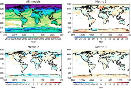
We examine the timing of passing temperature thresholds on the grid box scale to see whether performance-based model selection appreciably changes the timings. The spatial pattern of the timings of passing a temperature threshold for all models is examined. The impact of model selection is presented as the spatial pattern in the anomaly in timings for each performance-based selection relative to the all model timings.

The grid box timings of passing 2°C for the RCP4.5 simulations are in Figure 3 (top left panel) for all models. Analysis for RCP8.5 produces very similar results, and soﬁgures are provided in the supporting information (Figure S2 and Table S2). The very high latitudes pass 2°Cﬁrst (2000s–_{2010s) in RCP4.5 and are followed by} the rest of the land area (2020s to 2050s). The oceans pass 2°C later with most of the ocean having passed 2°C by the 2070s. Across the land, the pattern of when the warming crosses 2°C is consistent across both scenarios (RCPs). This is expected as we know that the pattern of warming over land is a relatively robust feature of most models, although the magnitude of warming especially in the high latitudes shows low agreement. This is evident in the relatively large spread in timings of warming (greater than 40 years) in the very high latitudes (see Figures S1 and S3, top left panel).

Over land, the use of metrics produces minimal change in the mean timings of passing 2°C and shows less than 10 year difference in the timing from the full ensemble. Over the ocean, the most signiﬁcant variation in timings is in the Southern Hemisphere with values of up to 30 years or more surrounding Antarctica. There are similar differences in the northern polar regions but not as spatially extensive and are shown in the standard deviation plots in Figures S1 and S3. This is expected as the differences in the magnitude of surface warming in polar regions have a high variability across CMIP5 models (Boe et al., 2009; Collins et al., 2013; Mahlstein & Knutti, 2012).

The spread across the models in the full ensemble, represented here as the standard deviation, is up to 25 years over land. Both metrics 1 and 2 show overall reductions of up 50%–_{75% in the spread (Figures S1} and S3). Some increases are seen in metric 2. The spread seen over land for metric 3 shows more of an even distribution of increases and decreases of up to 25%.

(9)

to 10 years of both later and earlier times. Over the oceans larger changes are seen in the Arctic regions of up to 25 years later (e.g., the Norwegian Sea) across all metrics.

The spread in timings of passing 4°C for RCP8.5 is shown in Figure S5 (top left panel) and is similar to those for SWL2 for RCP4.5, with values of up to 20 years spread over land and 10 years over the oceans. In contrast, the spread over the polar regions shows pockets of up to 50 years. These results imply that the metrics consid-ered in this paper do not change the mean timings of passing global SWLs and grid box-scale warming thresholds by greater than 10 years over land. However, the ranges seen in the timings are sensitive to model selection with the potential to reduce the spread in timings by up to 75%.

The distribution of the models’_{transient climate response (TCR) in the different ensembles may partially} explain the reduction in the ranges seen, as all metrics ensembles have a similar distribution centered around a TCR of 2°C compared to the unselected ensemble (see Figure S11). The possibility of a reduced spread in projected timings of passing temperature thresholds would be beneﬁcial in planning adaptation. However, if performance metrics are to be used, it is important to ensure adequate sampling of parameters known to be important in simulating the metrics of interest. This would give more conﬁdence in the reduction in the subselected ensemble spread being caused by the use of better performing models.

4.2. Selection Based On Bias Correction Techniques

[image:9.612.80.533.90.398.2]

Bias correction techniques try to improve theﬁdelity of climate projections and are used in impact studies to better estimate the potential consequences of a particular policy or environmental change. Throughout this section, the timings of passing SWLs derived from the uncorrected temperature simulations will be referred to as“_raw”_{timings and the timings derived from the bias-corrected temperature simulations are referred by} the bias correction technique (BC1, BC2, BC3, and BC4).

(10)

[image:10.612.80.535.90.396.2]

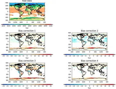
Figure 4.Timings of locally passing 4°C for CMIP5 simulations of RCP8.5 and the differences from applying metrics to sub-select CMIP5 models. The metrics are the same as those shown in Figure 3.

[image:10.612.109.505.478.701.2]

(11)

4.2.1. The Global Annual Mean Perspective

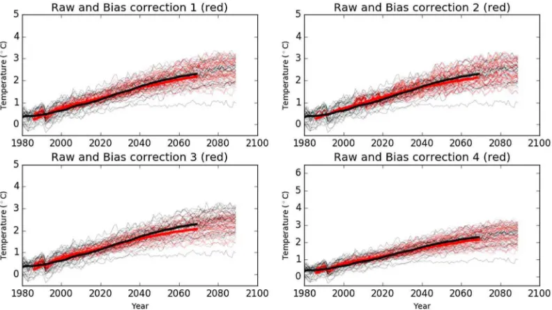
[image:11.612.108.505.87.310.2]

The impact of bias correction on the global annual mean temperature time series can be seen for RCP4.5 and RCP8.5 simulations in Figure 5. The raw temperature simulations are shown in black, while the bias-corrected simulations are given in red. The reduction in the spread of uncertainty (the thin red lines) in the temperature close to the baseline compared to the raw simulations is evident across all four bias corrections. However, the spread increases and resembles the raw simulations by the end of the century. This can be seen more clearly in Figure 6 where just the 10th–_{90th percentile range is shown.}

Figure 6.The uncertainty in the CMIP5 global annual mean temperature times series for the raw (black) and bias-corrected simulations (red) for RCP4.5. The 10th to 90th percentile range for the smoothed (20 years) time series is shown. The raw model data are in black, and the bias-corrected is given in red.

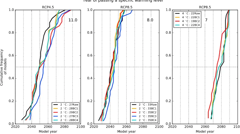
[image:11.612.108.501.460.681.2]

(12)

The timings of passing SWL2 for the raw simulations (black lines in Figure 5) result in a cumulative frequency (CF) which has a median year of 2050 and range from 2028 to 2081 for RCP4.5 (Figure 7, left). Applying the linear scaling method (BC1) to the simulations does not change the median value of passing SWL2. However, the range is shifted to later years, with the earliest crossing of SWL2 occurring later (2034) and the upper half of the distribution several years later. The second bias correction method (BC2), where the trend is added to the observations of present day, also does not affect the median year of passing SWL2, but the range has shifted to a few years later. The CF for the simple quantile mapping technique (BC3) appears the most different from of all bias correction techniques. The BC3 median year of passing SWL2 is shifted later to 2054, while the range is slightly reduced and shifted to later years (2039 to 2086). The trend-preserving quantile mapping technique (BC4) follows the linear scaling method (BC1) which is to be expected as on the global annual mean timescale they are similar in their methodology. The timings for passing SWL2 for RCP8.5 simulations (Figure 7, middle) for the raw and the bias correction techniques are closer in agreement with little difference in timings to the RCP4.5 simulations. The CF for the raw simulations has a median timing of passing SWL2 as 2042, the earliest passing at 2026, and last in 2055. The BC3 techni-que differs most from the raw CF and has a range in timing that is slightly larger and occurs later than the raw CF (2032 to 2066). The other bias correction techniques are about 4 to 5 years within the raw CF.

[image:12.612.75.535.93.446.2]

(13)

BC4 are 2 years earlier than for the raw CF, while for BC2 shows an earlier passing by 4 years. The simple quantile mapping technique (BC3) did not yield enough years to constitute a CF of greater than six models and therefore is not included here.

Overall, the bias correction techniques examined in this study lead to a reduction in spread in the bias-corrected temperature times series relative to the raw time series early in the 21st century but which converges with that of the raw time series by 2050s (Figures 5, 6, and also S6 where the 10th to 90th percen-tiles are shown). The resulting CFs for passing SWL2 show a narrower range (earliest to last year) or little change, except in the BC3 results for RCP8.5 where an increase seen. This is due to the reduced warming trend in the BC3 time series which results in the later timings of passing SWL2 (see Figure 5, bottom left column). The 10th to 90th percentile range in the CFs (Figure 6) is larger in the bias-corrected timings because the bias correction has slightly reduced the annual mean temperature rise in the latter half of the century (Figure 5). This results in later timings of passing the threshold than seen in the CF of the raw simulations. The SWL4 timings show little change in the range or median SWL4 year, with the exception of BC2 results where earlier timings of passing SWL4 are seen both in the earliest and median years and there is an increase in range. Therefore, the choice of bias correction technique can affect the magnitude of change in the range of SWL timings. While this study shows little change in the median timing of SWLs, the range in the timings can shift by up to 15 years.

4.2.2. Grid Box-Scale Impacts on the Timing of Temperature Thresholds

[image:13.612.75.535.92.446.2]

Here we show the impact of bias corrections on passing grid box-scale warming thresholds. If the anomaly in timings of passing a temperature threshold in a grid box is positive, then the timing based on the biased-corrected simulations is later than the timing based on the raw simulations.

(14)

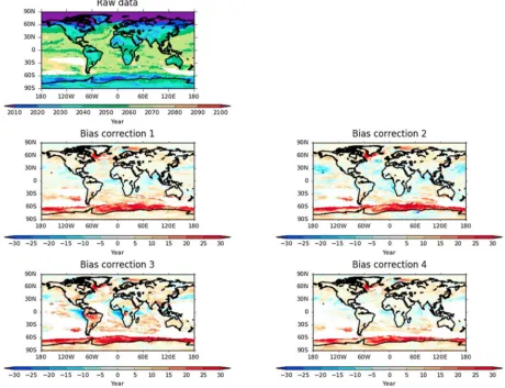
The raw grid box timings of passing 2°C for the RCP4.5 are shown in Figure 8 (Figure S8 shows similar results for RCP8.5 which are also summarized in Table S3). Land masses have reached 2°C by 2050, and the majority of the ocean reaches 2°C by the end of the 21st century. The grid box-scale timings for the four different bias correction techniques are in general later by 10 years over land than the raw timings, apart from BC3 which has timings of up to 30 years later. This suggests that bias correction techniques that are based on an offset or linear scaling (BC1, BC2, and BC4) do not affect the passing of temperature thresholds, compared to the timings derived from the raw simulations, by more than 10 years. Over the oceans, there are substantial differences in the grid box timings of the bias-corrected techniques compared to the raw timings especially in the Southern Ocean where the differences are up to 40 years later. This is a region where we expect differ-ences in warming between models related to uncertainty in future sea ice extent (e.g., see Figure S7). However, the magnitude of the difference might also be related to the proxy model data used for observed preindustrial temperatures in this work. The spread in timings across the bias correction techniques also shows an overall reduction over most land and oceans points and is most evident for the passing of 2°C. There are a few exceptions seen in the northern hemispheric tropical oceans and land. These are most pronounced for the BC2 timings for both 2°C and 4°C (Figure 9) and in the BC3 timings for 2°C. This increase in spread may be related to both BC2 and BC3 being constrained to the variability in temperature during the baseline period, albeit in different ways. The reduction in spread for 2°C is more pronounced where the timings occur early on in the 21st century (Figures 6 and S7). Only the BC3 timings show substantial differ-ence (in terms of being comparable to or larger than the standard deviation of the raw timings) over the ocean and in part over land in the mean timings of passing temperature thresholds. Areas in South America and Africa show the greatest difference in timings of passing 2°C and 4°C for BC3 compared to the raw data and the other bias correction techniques. This difference in timings is not surprising for BC3 as it is the bias correction method which corrects on the basis of the distribution of“_observed”_temperatures in the baseline period and is a method that markedly changes the warming trend in the temperature times series compared to the other three bias correction methods (see Figures 5 and S5).

[image:14.612.78.534.90.319.2]

The results here show that applying bias corrections to an ensemble of CMIP5 temperature simulations has the potential to affect the range in the timings of passing temperature thresholds. Particularly, if the tempera-ture threshold is crossed in the near term. The impact on the range of timings is scenario dependent on the global annual mean scale. The impact on the grid box scale is typically to reduce the range in the timings for near-term thresholds by up to 50% in some areas.

(15)

5. Discussion and Conclusions

This work explores the impact of approaches to reduce uncertainty in the timings of passing temperature thresholds both globally and locally. Two approaches are studied here:ﬁrst, selecting model ensembles based on a performance metric rather than assuming all models are equally likely and second, through the application of various bias correction techniques.

Using performance metrics to validate climate models can be a useful exercise in understanding the consequences of model development on projections of various types and an indication of model skill for present-day simulations. However, the use of these metrics for selecting models for a future projection is not straightforward unless the processes that are important to the change are dependent on the climate state. Nonetheless, in the absence of additional information, it could be viewed as a necessary condition for selection of models for future projections (Sanderson et al., 2015). Here we tried to assess if the bias from not selecting models based on common performance metrics would affect the timing of passing tempera-ture thresholds. On a global level, the three metrics (Figure 2) did not appear to change the year in which the temperature passed a threshold for the median model (a difference of within 10 years). This suggests that the metric selection has little impact on the median model year of passing SWLs for the performance metrics considered in this paper. In contrast, the range in timings of crossing SWL2 was affected and hence the uncer-tainty in the timing of thresholds. This could be because many quantities scale with temperature, so the use of performance metrics to subselect model reduces the range of model temperature responses (or TCR). There are indications of this here with metrics 1 and 2 leading to a reduced range in TCR and with metric 3 showing a similar range as the original model ensemble (Figure 2, top and middle rows). On the grid box scale and for the ensemble mean year of passing a temperature threshold, the metric-selected model ensem-bles show little change over land from the full model ensemble (less than 10 years) but show considerable variation over the oceans. The latter reﬂects the difference in the spatial pattern of warming from the differ-ent ensembles and is eviddiffer-ent from the larger spread represdiffer-ented by the standard deviation seen over the ocean than over land (see Figures S1 and S3). The main point illustrated by these results is that selecting model ensembles based on performance metrics can change the spread in the timings of passing SWLs. However, it is important to ensure that the known uncertainty in key parameters in simulating future climate change (e.g., those governing carbon cycle feedbacks) is sampled adequately in the selected ensemble. This would bring more conﬁdence to the model selection as the main cause of the reduction in uncertainty. Yet this would not address whether the metrics narrow the response for the right reason and highlights the need for the development of other complimentary approaches such as the application of emergent constraints (Cox et al., 2013; Qu & Hall, 2006; Wenzel et al., 2014).

Bias-correcting climate model data is common practice in impacts studies interested in absolute values of particular parameters and their changes above important thresholds. Here we studied whether both the application of bias correction and choice of bias correction technique would affect the timings of passing temperature thresholds. Four bias correction techniques in common usage were chosen. All four bias correc-tion techniques reduced the range of the global annual mean temperature rise seen in theﬁrst half of the century (see Figures 6 and S5). As a result, the uncertainty in initial conditions and model uncertainty are temporarily reduced by the bias correction but these uncertainties begin to grow with time and by the end of the century match the level of the uncorrected simulations. The quantile mapping technique changed the trend in the temperature time series, reﬂecting the differences in the nature of this bias correction technique compared to the other approaches. This correction uses a simple linear regression between the model simulation and observations as the form of the transfer function, and a different response might be expected if another relationship was used. The global annual mean cumulative frequencies of exceeding SWLs showed differences in the range of up to 10 years between the raw data and the corrected data timings. The impact of bias correction on the range appears here to be scenario dependent on the global annual mean level. For a scenario approaching stability the bias correction increases the 10th–_{90th percentile range} due to reduction in the annual mean temperature rise (Figure 5) resulting in later timings of SWL2.

(16)

timings over South America and central Africa (Figure 8, bottom left). All four bias correction techniques show a reduction in the spread of up to 50% in some regions compared to the raw data for the near-term passing of 2°C. In particular, the choice of bias correction used on the temperature time series can reduce the range in the timings of passing a warming threshold that has the potential to be reached by the middle of this century. In some cases, this is also true for the median year of passing the threshold (Figures S12 and S13).

Our mainﬁndings remain largely unchanged whether we look on the annual mean scale or a seasonal mean scale (see supporting information) for the performance-based model selection. The seasonal mean changes in timings due to the bias correction approaches are slightly larger in magnitude for parts of North America compared to the raw data. The bias correction results suggest that North American summers are warmer, and the winters are milder in a warming world. Consequently, the timings of passing 2°C in North America are earlier by up to 15 years in the summer and are similarly later in the winter (Figure S22). The reduction in the spread in the bias-corrected timings compared to the raw data is consistent with theﬁndings seen for the annual mean analysis.

The results of this seasonal analysis are of relevance to both the impact and adaptation community who systematically employ bias correction techniques in their work and who are concerned with the timing of crossing important thresholds in impact-related metrics. An effective adaptation strategy needs to account for climate uncertainty, especially for decisions with long lifetimes (e.g., major urban infrastructure and new irrigation projects). Decisions that are robust across a range of possible futures are recommended as part of a framework toward effective strategies (Dessai et al., 2009; Hallegatte, 2009; Wilby & Dessai, 2010). In addi-tion, adoptingﬂexible or reversible decisions that will allow for adjustments later are considered better adap-tation solutions (Hallegatte, 2009; Stafford Smith et al., 2011). For example, cities need to consider climate change in their decisions on planned buildings and housing developments (Hallegatte et al., 2011; Hallegatte & Corfee-Morlot, 2011; Rosenzweig et al., 2010). The timescales of such decisions are of the order of several decades (Stafford Smith et al., 2011). Therefore, for cities in North America the reduction in the spread of the projected warming or earlier timings of passing thresholds by 15 years may be an important consideration for the timescale of implementing factors in the built environment such as adequate ventila-tion and retroﬁtting air conditioning.

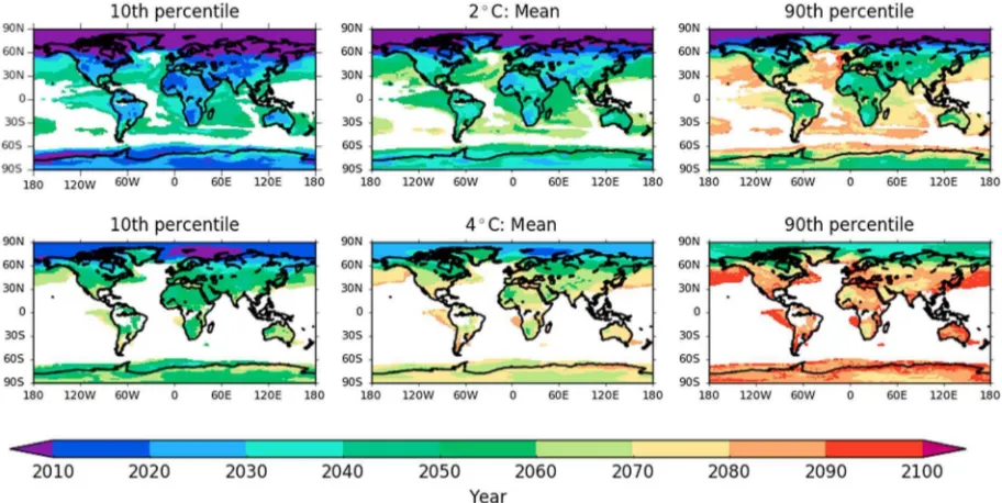
Our best estimate of the range and median timings of passing 2°C and 4°C locally are given in Figure 10 (top and bottom rows, respectively) and are based on the four bias correction techniques and the two forcing pathways examined here (only grid boxes where all four bias correction techniques show a passing year are shown). The mean model estimates most of the land passes 2°C by the 2050s, and 4°C is passed by the 2080s, while the 90th percentile estimates most of the land passing 2°C and 4°C by the 2080s and the end of the century, respectively.

This study shows that there is potential to reduce the uncertainty in the timings of passing near-term temperature thresholds by subselecting from model ensembles on the basis of performance metrics or the application of bias correction techniques. As these approaches can reduce the spread (by up to 50%) in the timings for speciﬁc warming levels at the grid box scale, caution is advised in planning climate change adaptation for locations where these potential reductions in timing uncertainty could affect decision making.

References

Adams, S., Baarsch, F., Bondeau, A., Coumou, D., Donner, R., Frieler, K.,…Warszawski, L. (2013).Turn down the heat: Climate extremes, regional impacts, and the case for resilience. Washington, DC: A report for the World Bank by the Potsdam Institute for Climate Impact Research and Climate Analytics.

Arnell, N. W., Hudson, D. A., & Jones, R. G. (2003). Climate change scenarios from a regional climate model: Estimating change in runoff in southern Africa.Journal of Geophysical Research,108(D16), 4519. https://doi.org/10.1029/2002JD002782

Barker, N. C., & Taylor, P. C. (2016). A framework for evaluating climate model performance metrics.Journal of Climate,29(5), 1773–_1782. https://doi.org/10.1175/JCLI-D-15-0114.1

Betts, R. A., Collins, M., Hemming, D. L., Jones, C. D., Lowe, J. A., & Sanderson, M. G. (2011). When could global warming reach 4°C? Philosophical Transactions of the Royal Society,369(1934), 67–84. https://doi.org/10.1098/rsta.2010.0292

Boe, J. L., Hall, A., & Qu, X. (2009). September sea-ice cover in the Arctic Ocean projected to vanish by 2100.Nature Geoscience,2(5), 341–_343. https://doi.org/10.1038/ngeo467

Clarke, L., Edmonds, J., Jacoby, H., Pitcher, H., Reilly, J., & Richels, R. (2007).Scenarios of greenhouse gas emissions and atmospheric concen-trations. Sub-report 2.1A of synthesis and assessment product 2.1 by the U.S. Climate change science program and the subcommittee on global change research(154 pp.). Washington, DC: Department of Energy, Ofﬁce of Biological & Environmental Research.

Collins, M., Knutti, R., Arblaster, J., Dufresne, J.-L., Fichefet, T., Friedlingstein, P.,…Wehner, M. (2013). Long-term climate change: Projections, commitments and irreversibility. In T. F. Stocker, et al. (Eds.),Climate change 2013: The physical science basis. Contribution of working group I

Acknowledgments

(17)

to theﬁfth assessment report of the intergovernmental panel on climate change(pp. 1029–_{1136). Cambridge, UK and New York: Cambridge} University Press.

Cox, P. M., Pearson, D., Booth, B. B., Friedlingstein, P., Huntingford, C., Jones, C. D., & Luke, C. M. (2013). Sensitivity of tropical carbon to climate change constrained by carbon dioxide variability.Nature,494(7437), 341–344. https://doi.org/10.1038/nature11882

Dee, D. P., Uppala, S. M., Simmons, A. J., Berrisford, P., Poli, P., Kobayashi, S.,…_{Vitart, F. (2011). The ERA-Interim reanalysis: Conﬁguration and} performance of the data assimilation system.Quartely Journal of the Royal Meteorological Society,137(656), 553–_{597. https://doi.org/} 10.1002/qj.828

Dessai, S., Hulme, M., Lempert, R., Pielke, R., & J. (2009). Do we need better predictions to adapt to a changing climate?Eos Transactions AGU, 90(13), 111–_{112. https://doi.org/10.1029/2009EO130003}

Dunne, J. P., Stouffer, R. J., & John, J. G. (2013). Reductions in labour capacity from heat stress under climate warming.Nature Climate Change, 3, 563–_{566. https://doi.org/10.1038/nclimate1827}

Ehret, U., Zehe, E., Wulfmeyer, V., Warrach-Sagi, K., & Liebert, J. (2012). HESS opinions“should we apply bias correction to global and regional climate model data?”_._{Hydrology and Earth System Sciences,}_{16(9), 3391}–_{3404. https://doi.org/10.5194/hess-16-3391-2012}

Field, C. B., Barros, V. R., Dokken, D. J., Mach, K. J., Mastrandrea, M. D., Bilir, T. E.,…_{White, L. L. (Eds.) (2014). IPCC, 2014: Summary for} pol-icymakers. InClimate change 2014: Impacts, adaptation, and vulnerability. Part A: Global and sectoral aspects. Contribution of working group II to theﬁfth assessment report of the intergovernmental panel on climate change(pp. 1–32). Cambridge, UK and New York: Cambridge University Press.

Flato, G., Marotzke, J., Abiodun, B., Braconnot, P., Chou, S. C., Collins, W.,…_{Rummukainen, M. (2013). Evaluation of climate models. In T. F.} Stocker, et al. (Eds.),Climate change 2013: The physical science basis. Contribution of working group I to theﬁfth assessment report of the intergovernmental panel on climate change(pp. 741–_{866). Cambridge, UK and New York: Cambridge University Press.}

Gleckler, P., Taylor, K., & Doutriaux, C. (2008). Performance metrics for climate models.Journal of Geophysical Research,113(D6), D06104. https://doi.org/10.1029/2007JD008972

Haerter, J. O., Hagemann, S., Moseley, C., & Piani, C. (2011). Climate model bias correction and the role of timescales.Hydrology and Earth System Sciences,15, 1065–_{1079. https://doi.org/10.5194/hess-15-1065-2011}

Hallegatte, S. (2009). Strategies to adapt to an uncertain climate change.Global Environmental Change,19, 240–_{247. https://doi.org/10.1016/} j.gloenvcha.2008.12.003

Hallegatte, S., & Corfee-Morlot, J. (2011). Understanding climate change impacts, vulnerability and adaptation at city scale: An introduction. Climatic Change,104(1), 1–12. https://doi.org/10.1007/s10584-010-9981-8

Hallegatte, S., Henriet, F., & Corfee-Morlot, J. (2011). The economics of climate change impacts and policy beneﬁts at city scale: A conceptual framework.Climatic Change,104(1), 51–_{87. https://doi.org/10.1007/s10584-010-9976-5}

Hawkins, E., Ortega, P., Suckling, E., Schurer, A., Hegerl, G., Jones, P.,…_{van Oldenborgh, G. J. (2017). Estimating change in global temperature} since the pre-industrial period.Bulletin of the American Meteorological Society. https://doi.org/10.1175/BAMS-D-16-0007.1,98(9), 1841–_1856.

Hawkins, E., Osborne, T. M., Ho, C. K., & Challinor, A. J. (2013). Calibration and bias correction of climate projections for crop modelling: An idealised case study over Europe.Agricultural and Forest Meteorology,170, 19–_{31. https://doi.org/10.1016/j.agrformet.2012.04.007} Hawkins, E., & Sutton, R. (2009). The potential to narrow uncertainty in regional climate predictions.Bulletin of the American Meteorological

Society,90(8), 1095–_{1107. https://doi.org/10.1175/2009BAMS2607.1}

Hawkins, E., & Sutton, R. (2016). Connecting climate model projections of global temperature change with the real world.Bulletin of the American Meteorological Society,97(6), 963–_{980. https://doi.org/10.1175/BAMS-D-14-00154.1}

Hempel, S., Frieler, K., Warszawski, L., Schewe, J., & Piontek, F. (2013). A trend-preserving bias correction—The ISI-MIP approach.Earth System Dynamics,4(2), 219–_{236. https://doi.org/10.5194/esd-4-219-2013}

Joshi, M., Hawkins, E., Sutton, R., Lowe, J., & Frame, D. (2011). Projections of when temperature change will exceed 2 °C above pre-industrial levels.Nature Climate Change,1(8), 407–_{412. https://doi.org/10.1038/nclimate1261}

Knutti, R. (2010). The end of model democracy?Climatic Change,102(3-4), 395–404. https://doi.org/10.1007/s10584-010-9800-2 Li, H., Shefﬁeld, J., & Wood, E. F. (2010). Bias correction of monthly precipitation and temperatureﬁelds from Intergovernmental Panel on

Climate change AR4 models using equidistant quantile matching.Journal of Geophysical Research,115, D10101. https://doi.org/10.1029/ 2009JD012882

Mahlstein, I., & Knutti, R. (2012). September Arctic sea ice predicted to disappear near 2°C global warming above present.Journal of Geophysical Research,117, D06104. https://doi.org/10.1029/2011JD016709

Masson, D., & Knutti, R. (2011). Climate model genealogy.Geophyiscal Research Letters,38, L08703. https://doi.org/10.1029/2011GL046864 Meehl, G. A., Stocker, T. F., Collins, W. D., Friedlingstein, P., Gaye, A. T., Gregory, J. M.,…_{Zhao, Z.-C. (2007). Global climate projections. In}

S. Solomon, et al. (Eds.),Climate change 2007: The physical science basis. Contribution of working group I to the fourth assessment report of the intergovernmental panel on climate change(pp. 748–_{845). Cambridge, UK and New York: Cambridge University Press.}

Milly, P. C. D., Betancourt, J., Falkenmark, M., Hirst, R. M., Kundzewicz, Z. W., Lettenmaier, D. P., & Stouffer, R. J. (2008). Stationarity is dead: Whither water management?Science,319(5863), 573–_{574. https://doi.org/10.1126/science.1151915}

Moss, R. H., Edmonds, J. A., Hibbard, K. A., Manning, M. R., Rose, S. K., van Vuuren, D. P.,…Wilbanks, T. J. (2010). The next generation of scenarios for climate change research and assessment.Nature,463(7282), 747–_{756. https://doi.org/10.1038/nature08823}

Oleson, J. E., Trnka, M., Kersebaum, K., Skjelvag, A., Seguin, B., Peltonen-Sainio, P.,…_{Micale, F. (2011). Impacts and adapation of} European crop production systems to climate change.European Journal of Agronomy,34(2), 96–_{112. https://doi.org/10.1016/j.} eja.2010.11.003

Piani, C., Weedon, G. P., Best, M., Gomes, S. M., Viterbo, P., Hagemann, S., & Haerter, J. O. (2010). Statistical bias correction of global simulated daily precipitation and temperature for the application of hydrological models.Journal of Hydrology,395(3–_{4), 199}–_{215. https://doi.org/} 10.1016/j.jhydrol.2010.10.024

Porter, J. R., Xie, L., Challinor, A. J., Cochrane, K., Howden, M., Iqbal, M. M.,…Travasso, M. I. (2014). Food security and food production systems. In Field, et al. (Eds.),Climate change 2014: Impacts, adaptation and vulnerability. Working group II contribution of working group II to theﬁfth assessment report of the intergovernmental panel on climate change(pp. 485–_{533). Cambridge, UK and New York: Cambridge University} Press.

Prudhomme, C., Giuntoli, I., Robinson, E. L., Clark, D. B., Arnell, N. W., Dankers, R.,…Wisser, D. (2014). Hydrological droughts in the 21st century, hotspots and uncertainties from a global multimodel ensemble experiment.Proceedings of the National Academy of Sciences, 111(9), 3262–_{3267. https://doi.org/10.1073/pnas.1222473110}

(18)

Raisanen, J., Ruokolainen, L., & Ylhaisi, J. (2010). Weighting of model results for improving best estimates of climate change.Climate Dynamics,35(2–_{3), 407}–_{422. https://doi.org/10.1007/s00382-009-0659-8}

Reichler, T., & Kim, J. (2008). How well do coupled models simulate today’_{s climate?}_{Bulletin of the American Meteorological Society,}_89(3), 303–311. https://doi.org/10.1175/BAMS-89-3-303

Reifen, C., & Toumi, R. (2009). Climate projections: Past performance no guarantee of future skill?Geophysical Research Letters,36, L137704. https://doi.org/10.1029/2009GL038082

Riahi, K., Grubler, A., & Nakicenovic, N. (2007). Scenarios of long-term socio-economic and environmental development under climate sta-bilization.Technological Forecasting and Social Change,74(7), 887–935. https://doi.org/10.1016/j.techfore.2006.05.026

Rosenzweig, C., Solecki, W., Hammer, S. A., & Mehrotra, S. (2010). Cities lead the way in climate-change action.Nature,467, 909–_{911. https://} doi.org/10.1038/467909a

Sanderson B. M. & Knutti, R. (2012). On the interpretation of constrained climate model ensembles.Geophysical Research Letters,39, L16708. https://doi.org/10.1029/2012GL052665

Sanderson, B. M., Knutti, R., & Caldwell, P. (2015). A representative democracy to reduce interdependency in a multi-model ensemble.Journal of Climate,28, 5171–_{5194. https://doi.org/10.1175/JCLI-D-14-00362.1}

Schleussner, C. F., Lissner, T. K., Fischer, E., Wohland, J., Perrette, P., Golly, A.,…_{Schaeffer, M. (2016). Differential climate impacts for} policy-relevant limits to global warming: The case of 1.5°C and 2°C.Earth System Dynamics,7(2), 327–351. https://doi.org/10.5194/esd-7-327-2016

Smith, S. J., & Wigley, T. M. L. (2006). Multi-gas forcing stabilization with the MiniCAM.Energy Journal,27, 373–_391.

Solomon, S., Qin, D., Manning, M., Chen, Z., Marquis, M., Averyt, K.,…_{Miller, H. L. (2007). Climate change 2007: The physical science basis. In} Contributions of working group I to the fourth assessment report of the IPCC(996 pp.). Cambridge, UK and New York: Cambridge University Press.

Stafford Smith, M., Horrocks, L., Harvey, A., & Hamilton, C. (2011). Rethinking adaptation for a 4°C world.Philosophical Transactions of the Royal Society A,369, 196–_{216. https://doi.org/10.1098/rsta.2010.0277}

Stocker, T. F., Qin, D., Plattner, G.-K., Tignor, M., Allen, S. K., Boschung, J.,…_{Midgley, P. M. (2014).}_{Climate change 2013: The physical science} basis: Working group I contribution to theﬁfth assessment report of the intergovernmental panel on climate change. Cambridge, UK and New York: Cambridge University Press.

Taylor, K. E., Stouffer, R. J., & Meehl, G. A. (2012). An overview CMIP5 and the experiment design.Bulletin of the American Meteorological Society,93(4), 485–498. https://doi.org/10.1175/BAMS-D-11-00094.1

Tebaldi, C., & Knutti, R. (2007). The use of the multi-model ensemble in probabilistic climate projections.Philosophical Transactions of the Royal Society,A365, 2053–_2075.

Teutschbein, C., & Seibert, J. (2012). Bias correction of regional climate model simulations for hydrological climate-change impact studies: Review and evaluation of different methods.Journal of Hydrology,456-457, 12–29. https://doi.org/10.1016/j.jhydrol.2012.05.052 Themeßl, M. J., Gobiet, A., & Heinrich, G. (2012). Empirical-statistical downscaling and error correction of regional climate models and its

impact on the climate change signal.Climatic Change,112(2), 449–_{468. https://doi.org/10.1007/s10564-011-0224-4}

Themeßl, M. J., Gobiet, A., & Leuprecht, A. (2011). Empirical-statistical downscaling and error correction of daily precipitation from regional climate models.International Journal of Climatology,31(10), 1530–1544. https://doi.org/10.1002/joc.2168

United Nations / Framework Convention on Climate Change (2015). Adoption of the Paris Agreement, 21st Conference of the Parties, Paris: United Nations.

Watanabe, S., Kanae, S., Seto, S., Yeh, P. J. F., Hirabayashi, Y., & Oki, T. (2012). Intercomparison of bias correction methods for monthly tem-perature and precipitation simulated by multiple climate models,Journal of Geophysical Research,117, D23114. https://doi.org/10.1029/ 2012JD018192

Watterson, I. G., Bathols, J., & Heady, C. (2014). What inﬂuences the skill of climate models over the continents?Bulletin of the American Meteorological Society,95, 689–_{700. https://doi.org/10.1175/BAMS-D-12-00136.1}

Wenzel, S., Cox, P. M., Eyring, V., & Friedlingstein, P. (2014). Emergent constraints on climate-carbon cycle feedbacks in the CMIP5 Earth system models.Journal of Geophysical Research: Biogeosciences,119, 794–_{807. https://doi.org/10.1002/2013JG002591}

Wilby, R. L., & Dessai, S. (2010). Robust adaptation to climate change.Weather,65(7), 180–_{185. https://doi.org/10.1002/wea.543}

Wise, M. A., Calvin, K., Thomson, A., Clarke, L., Bond-Lamberty, B., Sands, R.,…_{Edmonds, J. (2009). Implications of limiting CO2 concentrations} for land use and energy.Science,324(5931), 1183–_{1186. https://doi.org/10.1126/science.1168475}