Nonlinear projection filter for target tracking using range sensor & optical tracker

This is a repository copy of Nonlinear projection filter for target tracking using range

sensor & optical tracker.

White Rose Research Online URL for this paper:

http://eprints.whiterose.ac.uk/100531/

Version: Accepted Version

Proceedings Paper:

Kim, J orcid.org/0000-0002-3456-6614 (2016) Nonlinear projection filter for target tracking

using range sensor & optical tracker. In: IFAC-PapersOnLine. 20th IFAC Symposium on

Automatic Control in Aerospace - ACA 2016, 21-25 Aug 2016, Sherbrooke, Quebec,

Canada. Elsevier , pp. 438-443.

https://doi.org/10.1016/j.ifacol.2016.09.075

© 2016, IFAC (International Federation of Automatic Control) Hosting by Elsevier Ltd. All

rights reserved. This is an author produced version of a paper published in

IFAC-PapersOnLine. Uploaded in accordance with the publisher's self-archiving policy.

[email protected] https://eprints.whiterose.ac.uk/

Reuse

Unless indicated otherwise, fulltext items are protected by copyright with all rights reserved. The copyright exception in section 29 of the Copyright, Designs and Patents Act 1988 allows the making of a single copy solely for the purpose of non-commercial research or private study within the limits of fair dealing. The publisher or other rights-holder may allow further reproduction and re-use of this version - refer to the White Rose Research Online record for this item. Where records identify the publisher as the copyright holder, users can verify any specific terms of use on the publisher’s website.

Takedown

If you consider content in White Rose Research Online to be in breach of UK law, please notify us by

Nonlinear projection filter for target

tracking using range sensor & optical

tracker

⋆

Jongrae Kim∗

∗_{Institute of Design, Robotics & Optimisation (iDRO), School of} Mechanical Engineering, University of Leeds, Leeds LS2 9JT, UK

(e-mail: [email protected])

Abstract: Target tracking filters have a variety of applications in various areas. Typically, a radar provides the range measurement and an optical sensor measures the orientation of a target. The measurements provided by the sensors have very strong nonlinearities with the states of the target given in the Cartesian coordinates while its dynamics is linear parameter time-varying. The time-varying component exists because of the unknown acceleration input in the target. Nonlinear projection filter provides a solution to the nonlinear estimation problem by approximating the solution as a linear combination of orthogonal basis functions. The analytic expression for propagating the joint probability density function is derived for the target tacking problem and this reduces large amount of computation times, where the filter equations are normally obtained numerically. The effectiveness of the filter is demonstrated by a numerical simulation.

Keywords:Nonlinear estimation, Nonlinear projection filter, Target tracking

1. INTRODUCTION

Moving target tracking has been studied extensively in the past and it has many areas of applications for tracking various moving objects such as aircraft (Spingarn and Weidemann, 1972), ships (Chen and Huang, 2013), mobile robots (Benavidez and Jamshidi, 2011). One of the earliest studies includes α-β filter (Rogers, 1987), α-β-γ filter (Gray and Murray, 1993) derived from the steady-state Kalman filter (Kalman, 1960). A stability analysis of α

-β-γ filter is shown in Tenne and Singh (2002). Target tracking using particle filter is shown in Gustafsson et al. (2002). A good survey of the target tracking problem for various types of acceleration models is found in Li and Jilkov (2003).

One of the main difficulties in target tracking filter design stems from its strong nonlinearities in the measurement equation. The range measurements from a radar and the azimuth/elevation angles from an optical tracker are typical sensor outputs in the target tracking problems. These measurements have strong nonlinear relations with a Cartesian coordinates dynamics of the moving target (Park, 1999).

Nonlinear projection filter solves the nonlinear estimation problem directly from the Fokker-Planck equation (Beard et al., 1999). The Fokker-Planck equation is in general difficult to solve in real-time because of its high compu-tational demand. Nonlinear projection filter provides the way to reduce the computational complexity through the

⋆ _{This research is supported by EPSRC Research Grant,}

EP/N010523/1, Balancing the impact of city infrastructure engineer-ing on natural systems usengineer-ing robots.

approximation of the solution as a linear combination of a set of orthogonal basis functions. Recently, the filter is further improved so that it requires less computation and fits better to an array of parallel sensors and parallel computation in (Single-Liertz et al., 2015).

In the following, firstly, a target tracking problem is intro-duced in terms of its dynamics and measurement equation; secondly, the nonlinear projection filter is summarised; thirdly, the filter is developed for the target tracking; fourthly, simulation results are discussed; and finally, con-clusions are presented.

2. TARGET TRACKING

2.1 Dynamics & Measurements

A target dynamics for each axis can be written as follows:

d dt

"_r

˙

r wr

#

=

" _r˙

−τr˙+u+wr

−αwr #

+

"₀

0 1

#

v (1)

where r is equal to x,y or z, which is the component of each direction in the Cartesian coordinates, d/dt is the time derivative,ris the position of the target in the given axis, ˙r is the time derivative of r, τ is the target drag coefficient in r-direction, uis the target control input in

r-direction, which is in the known bound in [u,u¯], wr is

the uncertainty in the target acceleration (Singer, 1970),

αis the inverse of the manoeuvre time constant, andv is zero-mean white noise Gaussian with the variance,σ2

v. Or,

in a compact form

x

y

z

Fig. 1. Tracking coordinates,x,y, andz, and the measure-ments, range,ρ, elevation,φ, and azimuth,θ

x=

"_r

˙

r w

#

, A=

"_{0 1 0}

0 −τ 1 0 0 −α

#

,u=

"₀

u

0

#

, G=

"₀

0 1

#

, (3)

and E(β2_{) =σ}2

vdt.

The measurement given by a range sensor and an optical tracker are

yk = "_ρ

k

φk

θk #

=h(xk) +vk (4)

where each component of the measurement represents the range measurement from radar, ρk, the elevation, ψk,

and the azimuth, θk, measurements from optical trackers,

respectively, as shown in Figure 1. And, they satisfy the following equations with the Cartesian coordinates:

h(xk) = 

      

q

x2

k+yk2+zk2

tan−1 ₋ zk p

x2

k+yk2 !

tan−1 _y

k

xk



      

, vk= "_v

ρ

vφ

vθ #

(5)

and xk, yk, zk are the Cartesian coordinates at the

k-th sampling time. Note that (1) can be discretised and the filtering problem is considered purely in the discrete domain together with the discrete measurement, (4). Without introducing the discrete approximation, the original continuous-discrete mixed filter problem is to be solved.

2.2 Nonlinear projection filter

For a standard form of nonlinear stochastic differential equation given in (2) with a fixed u, the corresponding joint pdf (Probability Density Function), p(t,x), follows the Fokker-Planck equation given by

∂p ∂t =−

n X

i=1 ∂(pfi)

∂xi

+1 2

n X

i=1

n X

j=1

∂2h_{p GQG}T i,j

i

∂xi∂xj

(6)

where xi and fi are i-th element of the n-dimensional

vectorsx andf(x, u), respectively, (GQGT₎

i,j isi-th row

and j-th column element of the matrix,GQGT_{, andQis}

equal toσ2

v.

The nonlinear projection filter assumes that the joint pdf has the following form:

p(t,x) =cT(t)φ(x) (7) where c is a time-varying vector, whose dimension is

Np, and φ is Np-dimensional vector, whose elements

form a set of orthogonal basis functions. Substituting the approximation into the Fokker-Planck equation gives the propagation equation forc(t).

Substituting the approximation into the following Bayes’ theorem, (Arulampalam et al., 2002), provides the update equation forc(t):

p(t+_k,x_|Yk) =η p(yk|x)p(t−k,x|Yk−1) (8)

whereη is the normalising constant,p(yk|x) is the sensor

model.

The full details on the derivation of nonlinear projection filter for a general form of nonlinear equation can be found in Beard et al. (1999).

2.3 Filter Model & Basis Functions

Not all parameters in the target dynamics shown in (1) are known perfectly and they might change with time, for example, depending on the acceleration input, u, or the manoeuvre profile given by α. It is, hence, that the following simpler equation would be more attractive in deriving the projection filter:

d

r

˙

r

=

˙

r ur

dt+

0 1

dγ (9)

where ur is a priori estimated acceleration bound for a

given target and E(γ2_{) =σ}2

γdt, andσγ2 is the variance.

In the projection filter, the pdf is approximated by a finite sum of basis functions as follows:

p(t, r,r˙)≈cT_r(t)φ(r,r˙) (10)

wherecr(t) is anN2-dimensional time-varying vector, (·)T is the transpose,

φ(r,r˙) =ξ(r)⊗ξ( ˙r) (11)

⊗is the Kronecker product,ξ(s) is aN-dimensional vector fors=ror ˙r. Thei-th component of ξ(s) is the element of a set of orthogonal basis functions as follows:

ξi(s) =  



1/p∆s fori= 1,

r

2 ∆s

cos [κ(i)(s−as)] for 2≤i≤Ns

(12)

where ∆sis equal tobs−as,asis the lower bound ofs,bs

is the upper bound ofs, i.e.,s∈[as, bs],Nsis the number

of basis functions, and

κs(i) =

(i−1)π

∆s

(13)

In addition, ξi(s) satisfies the following orthogonality

condition:

Z bs

as

ξi(s)ξj(s)ds=

1 fori=j,

0 fori6=j (14)

fori, j= 1,2,3, . . . , Ns.

ξ′(s) = dξ(s)

ds =−

r 2 ∆s       0

κs(2) sin[κs(2)(s−as)]

κs(3) sin[κs(3)(s−as)]

.. .

κs(N) sin[κs(N)(s−as)]       (15)

and in a compact form,

ξ′(s) =−Ksψ(s) (16)

where

Ks= diag [κs(1) κs(2) . . . κs(N)], (17a)

ψ(s) =

r 2 ∆s       0

sin[κs(2)(s−as)]

sin[κs(3)(s−as)]

.. .

sin[κs(N)(s−as)]       , (17b)

and diag[. . .] is the diagonal matrix, whose diagonal terms are given in the bracket. In addition, the second derivative can be easily shown to equal to the followings:

ξ′′(s) = d

dsξ

′

(s) =−_dsdKsψ(s)

=− r 2 ∆w K2       0

cos[κs(2)(s−as)]

cos[κs(3)(s−as)]

.. .

cos[κs(N)(s−as)]      

=−K2

s                1 √ ∆s r 2 ∆s

cos[κs(2)(s−as)] r

2 ∆s

cos[κs(3)(s−as)]

.. .

r

2 ∆s

cos[κs(N)(s−as)]                (18)

where the first element is zero asκ(1) = 0. Hence,

ξ′′(s) =−Ks2ξ(s) (19)

2.4 Propagation: target position & velocity

Apply the Fokker-Planck equation to (9)

∂p(t, r,r˙)

∂t =−

∂[p(t, r,r˙) ˙r]

∂r −

∂[p(t, r,r˙)ur]

∂r˙

+1 2

∂2_{[p(t, r,r˙)σ}

α]

∂r˙2 (20)

Substitute (10) with (11) into (20)

˙

cT_r[ξ(r)⊗ξ( ˙r)] = ˙rcT_r[Krψ(r)⊗ξ( ˙r)]

+ur cTr[ξ(r)⊗K˙rψ( ˙r)]

−σ

2

α

2 c

T

r[ξ(r)⊗Kr2˙ξ( ˙r)] (21)

Multiply [ξ(r) ⊗ ξ( ˙r)]T _{both sides and integrate over}

r∈[ar, br] and ˙r∈[ar˙, br˙]

˙

cr(t) =

Z Z

[ξ(r)⊗ξ( ˙r)][Krψ(r)⊗r˙ξ( ˙r)]T (22)

+ur [ξ(r)⊗ξ( ˙r)][ξ(r)⊗Kr˙ψ( ˙r)]T

−σ

2

α

2 [ξ(r)⊗ξ( ˙r)][ξ(r)⊗K

2 ˙

rξ( ˙r)]T

drdv˙ cr(t)

Using the following identities

(A⊗B)(C⊗D) = (AC)⊗(BD) (23a) (A⊗B)T _=AT _⊗BT _(23b)

where all dimensions are appropriate for the matrix mul-tiplication,

˙

cr(t) =

Z

[ξ(r)KrψT(r)]dr⊗ Z

[ ˙rξ( ˙r)ξT( ˙r)]dr˙

+ur IN ⊗ Z

[ξ( ˙r)Kr˙ψT( ˙r)]dr˙− σ2

α

2 IN ⊗K

2 ˙

r

cr(t)

=A(ur)cr(t) (24)

where A(ur) is N2-dimensional square matrix, which is

defined by the terms inside the bracket in front of c(t) in the right hand side of the equation. The discrete time transition equation is given by

cr(tk+1) = Φ(tk+1, tk, ur)cr(tk) (25)

where

Φ(tk+1, tk, ur) =eA(ur)∆tk, (26)

and ∆tk=tk+1−tk. Note that the transition matrix can

be calculated off-line and stored in on-board computer for a finite set of samples ofur in [ur,u¯r].

The integrations in (24) have analytic expressions. For brevity, all the integrations from now on are assumed to be performed over the appropriate sampling space such thats∈[as, bs], wheres=r, or ˙r, or indicated otherwise.

For i≥ 2,j ≥2 and i 6=j, the ith-row and jth-column element of

Z

[ ˙rξ( ˙r)ξT( ˙r)]dr˙

ijorji

(27)

=

 



0, for bothi, j even or odd

−2∆_π2r˙

₁

(i−j)2 +

1 (i+j−2)2

, otherwise

or fori= 1 and j >1, i.e. the first row elements,

Z

[ ˙rξ( ˙r)ξT( ˙r)]dr˙

1j =   

0, forj is odd −2√2∆r˙

π2_(j−1)2, otherwise

(28)

and the first column elements are of the same form, and fori=j andi∈[1, N],

Z

[ ˙rξ( ˙r)ξT( ˙r)]dr˙

ii

= ar˙+br˙

2 (29)

In addition, for alliin [1, N],

Z

[ξ(s)KψT(s)]ds

i1

= 0 (30)

i.e, the first column elements are all zero, wheresis equal toror ˙r. The first row elements forj∈[2, N] are equal to

Z

[ξ(s)KψT(s)]ds

1j =   

0, forj odd 2√2

∆s

All diagonal terms, for i =j, are zero. Finally, for i6= j

andi, j∈[2, N],

Z

[ξ(s)KψT(s)]ds

ij

=j−1 ∆s

cos(i−j)π−1

i−j

+cos(i+j−3)π+ 1

i+j−2

and it becomes

Z

[ξ(s)KψT(s)]ds

ij

(32)

= j−1 ∆s

 



0, for bothi, j even or odd

−_(i 2 −j)+

2

(i+j−2), otherwise

The same form of update equations for y or z-axis, i.e.,

cy(t) andcz(t), can be derived from the same procedures.

2.5 Update: target position & velocity

The full joint pdf for all three Cartesian axes has to be considered to obtain an update algorithm. Let

p=p(x,x˙)p(y,y˙)p(z,z˙) (33) = [cT_x(t)φ(x,x˙)][cT_y(t)φ(y,y˙)][cT_z(t)φ(z,z˙)] where the joint pdf is multiplication of all three joint pdfs for three axes, which are assumed to be statistically independent to each other.

Substitute (33) into the Bayesian update equation, (8),

cT_x(t+_k) [ξ(x)⊗ξ( ˙x)]

cT_y(t+_k) [ξ(y)⊗ξ( ˙y)]

cT_z(t+_k) [ξ(z)⊗ξ( ˙z)]

=ηx p(yk|r)

cT_x(t−

k) [ξ(x)⊗ξ( ˙x)] (34)

cT_y(t−

k) [ξ(y)⊗ξ( ˙y)]

cT_z(t−

k) [ξ(z)⊗ξ( ˙z)]

where ηx is the normalising constant to be determined, andrincludes all three coordinates,x,y, andz. Integrate both sides by all parameters except xand ˙xand the left hand side (LHS) of the equation becomes

(LHS) =cTx(t+k) [ξ(x)⊗ξ( ˙x)] (35)

as the integrations of the other two brackets are simply equal to 1. In addition, the term inside the second bracket in the right hand side (RHS) of the update equation becomes

cT_y(t− k)

"

ξ(y)⊗

Z by˙

ax˙

ξ( ˙y)dy˙

#

(36)

=cT_y(t− k)           

ξ(y)⊗

      p

∆y˙

0 0 .. . 0                  =p

∆y˙cTy(t−k)ξ(y)

where cy(t−_k) is the N-dimensional vector constructed by

every Nth-element from the first to N2-th elements in

cy(t−_k). The similar steps can apply to the third term as follows:

cT_z(t− k)

"

ξ(z)⊗

Z bz˙

az˙

ξ( ˙z)dz˙

#

=p∆z˙cTz(t−k)ξ(z) (37)

Hence,

cT_x(t+_k) [ξ(x)⊗ξ( ˙x)] =η

Z Z

p(y_k|r)[cT_y(t− k)ξ(y)]

[cT_z(t−

k)ξ(z)] dydz

cT_x(t−

k) [ξ(x)⊗ξ( ˙x)] (38)

where √∆r˙ and

√

∆z˙ are absorbed in the normalising

constant,ηx.

Multiply [ξ(x)⊗ξ( ˙x)]T _{both sides and integrate over the}

sampling spaces, respectively,

cTx(t+k) = Z Z Z Z

p(yk|r)[cTy(t−k)ξ(y)][c T

z(t−k)ξ(z)] dydz n

cT_x(t−

k) [ξ(x)⊗ξ( ˙x)] [ξ(x)⊗ξ( ˙x)]

To_{dxdx η˙}

x (39)

Again using the Kronecker product identity, the update equation becomes

cx(t+_k) =ηxBxcx(t−_k) (40) where

Bx=

Z Z Z

p(yk|r)[cTy(t−k)ξ(y)][cTz(t−k)ξ(z)]

h

ξ(x)ξT(x)i⊗IN o

dxdydz (41)

Note thatBxis symmetric.

The normalising constant is determined by the fact that the pdf must be equal to 1 after it is integrated over the sampling space.

Z Z

cT_x(t+_k) [ξ(x)⊗ξ( ˙x)]dxdx˙ (42)

=ηx cTx(t−k)Bx

Z Z

[ξ(x)⊗ξ( ˙x)]dxdx˙ = 1 (43)

Then,

ηxcTx(t−k)Bx

                 p ∆x 0 0 .. . 0       ⊗       p

∆x˙

0 0 .. . 0                 

= 1 (44)

Therefore,

ηx=

1 √

∆x∆x˙

cT

x(t−k)bx1

(45)

wherebx1 is the first column ofBx.

Similarly, the update equations forcy(t+_k) andcz(t+_k) are obtained as follows:

cy(t+_k) =ηyBycy(t−_k) (46a)

cz(t+_k) =ηzBzcz(t−_k) (46b) where

By=

Z Z Z

p(yk|r)[cTx(t−k)ξ(x)][c T

z(t−k)ξ(z)] h

ξ(y)ξT(y)i⊗IN o

dxdydz (47a)

Bz=

Z Z Z

p(yk|r)[cTx(t−k)ξ(x)][c T

y(t−k)ξ(y)] h

ξ(z)ξT(z)i⊗IN o

Fig. 2. Velocity history: each segment of the straight line corresponds to a 3g-turn.

and the normalising constant for each is defined by

ηy =

1

p

∆y∆y˙cyT(t−k)by1

(48a)

ηz=

1 √

∆z∆z˙czT(t−k)bz1

(48b)

3. NUMERICAL SIMULATIONS

Initially, a target is at x = 2.0km, y = 0.7km, and

z = 0km with the initial velocity is equal to 50m/s, 50m/s and 30m/s in x, y, and z direction, respectively. The drag coefficient, τ, is equal to 0.01. The manoeuvre time constant,α−1_{, is set to 10s. The variance,σ}2

v, is equal

to 0.01 (Park, 1999). The acceleration input,u, is between ±30 m/s2_.

Figure 2 shows the velocity histories of the target and the corresponding trajectory is shown in Figure 3 indicated by the solid blue line. The manoeuvre is composed of several 3g-turns during 20 seconds.

In the model for the projection filter, ur is in the range

of ± 33 m/s, i.e., 10% margin to the actual range of acceleration. The variance of the process noise in the model, σ2

γ is set to 0.01. The number of basis function

for each state, N, is set to 15. Hence, the dimension of

A(ur) for the propagation in the filter is 225 (=15×15).

The acceleration input, ur, in the model is not measured

directly. Possibly choose several candidateurin the range

and run multiple filters at the same time. On the other hand, physically the position and the velocity will be confined in an envelop by two extreme possible position and velocity trajectories, which are resulted from two extreme acceleration input, i.e., ur = −33 or ur = 33,

respectively.

The sensor model is assumed to be of the normal distribu-tion as follows:

p(yk|x) =

e−

1

2[yk−h(x)]T_R−1

k [yk−h(x)]

p

(2π)3_|R

k|

,

whereRk= E(vkvkT), which is assumed to be constant as

follows (Park, 1999):

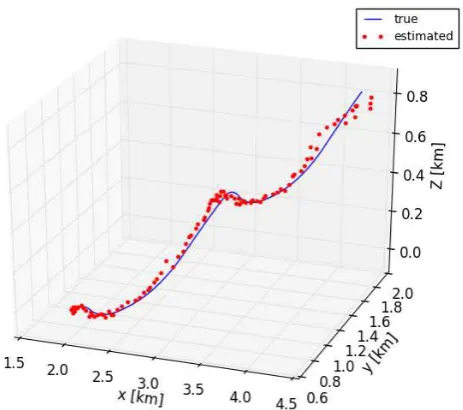
Fig. 3. Target trajectory in the Cartesian coordinates: the true in blue solid line and the estimated in red dots

Rk= diag

(7.5 [m])2 (0.002 [rad])2 (0.002 [rad])2

(49) The measurement is available every 0.02s and this is relatively higher frequency compared to the given range of acceleration range. As a result, the position estimation based on the maximum acceleration and the one based on the minimum acceleration does not make any significant difference.

The mean value or the expected value of the position based on the estimation of joint pdf is shown in Figure 3 indicated in the red dots, where the mean value of the position is calculated as follows:

E[x(tk)] = Z bx

ax

xp(x)dx=

Z bx

ax

cx(t+k)ξ(x)dx (50)

where [ax, bx] is equal to [1.0,6.4]km. Similarly, for the

estimate ofy(tk) andz(tk) are calculated, where [ay, by] =

[0.35,2.84]km and [az, bz] = [0,2.25]km. The position

esti-mation error in the average sense is shown in Figure 4. The maximum error occurs inx-direction, whose magnitude is about 250m.

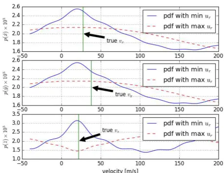
Similarly, the mean estimation of velocity can be calcu-lated but the velocity estimation error in the mean sense is in general very poor. The estimated joint pdf attk= 20s

for the velocity is shown in Figure 5. Two joint pdfs for the velocity based on two different accelerations are very different. Unlike Kalman filter, which tracks only the first two moments, the projection filter tracks whole joint pdf as shown in Figure 5. Additional information from the joint pdf could be used to optimally select source of the measurements or place the position of sensors in order to improve the accuracy of the pdf.

4. CONCLUSIONS

per-Fig. 4. Position estimation error for each direction

Fig. 5. Estimated velocity joint pdf with maximum or minimum acceleration assumption attk= 20s

formance of the algorithm is demonstrated with a realistic target tracking scenario where a radar sensor provides the range measurement and an optical sensor provides the azimuth and the elevation angles measurements. Thorough comparisons with existing nonlinear filtering algorithms would be performed in future to reveal possible advantages and disadvantages of the proposed filtering algorithm.

ACKNOWLEDGEMENTS

This research is supported by EPSRC Research Grant, EP/N010523/1, Balancing the impact of city infrastruc-ture engineering on natural systems using robots. The author thank YongKyu Park in KARI (Korea Aerospace Research Institute) in Daejeon, South Korea for introduc-ing the target trackintroduc-ing problem.

REFERENCES

Arulampalam, M.S., Maskell, S., Gordon, N., and Clapp, T. (2002). A tutorial on particle filters for online nonlinear/non-Gaussian Bayesian track-ing. Signal Processing, IEEE Transactions on, 50(2), 174–188. doi:10.1109/78.978374. URL

http://dx.doi.org/10.1109/78.978374.

Beard, R., Kenney, J., Gunther, J., Lawton, J., and Stir-ling, W. (1999). Nonlinear Projection Filter Based on Galerkin Approximation. Journal of Guidance, Con-trol, and Dynamics, 22(2), 258–266. doi:10.2514/2.4403. URLhttp://dx.doi.org/10.2514/2.4403.

Benavidez, P. and Jamshidi, M. (2011). Mobile robot navi-gation and target tracking system. InSystem of Systems Engineering (SoSE), 2011 6th International Conference on, 299–304. doi:10.1109/SYSOSE.2011.5966614. Chen, S. and Huang, W. (2013). Target tracking

us-ing particle filter with x-band nautical radar. In

Radar Conference (RADAR), 2013 IEEE, 1–6. doi: 10.1109/RADAR.2013.6585993.

Gray, J. and Murray, W. (1993). A derivation of an analytic expression for the tracking index for the alpha-beta-gamma filter. Aerospace and Electronic Sys-tems, IEEE Transactions on, 29(3), 1064–1065. doi: 10.1109/7.220956.

Gustafsson, F., Gunnarsson, F., Bergman, N., Forssell, U., Jansson, J., Karlsson, R., and Nordlund, P.J. (2002). Particle filters for positioning, navigation, and tracking.

Signal Processing, IEEE Transactions on, 50(2), 425– 437. doi:10.1109/78.978396.

Kalman, R.E. (1960). A new approach to linear filtering and prediction problems.Journal of Basic Engineering, 82, 35–45.

Li, X. and Jilkov, V. (2003). Survey of maneuvering target tracking. part i. dynamic models. Aerospace and Electronic Systems, IEEE Transactions on, 39(4), 1333– 1364. doi:10.1109/TAES.2003.1261132.

Park, Y.K. (1999). An improvement of target track-ing algorithm ustrack-ing multiple model adaptive estimator. MSc Thesis, Aerospace Engineering, Inha University, Incheon, Republic of Korea, in Korean.

Rogers, S. (1987). Alpha-beta filter with correlated measurement noise. Aerospace and Electronic Sys-tems, IEEE Transactions on, AES-23(4), 592–594. doi: 10.1109/TAES.1987.310893.

Singer, R.A. (1970). Estimating optimal tracking filter per-formance for manned maneuvering targets. Aerospace and Electronic Systems, IEEE Transactions on, AES-6(4), 473–483. doi:10.1109/TAES.1970.310128.

Single-Liertz, T., Kim, J., and Richardson, R. (2015). Nonlinear projection filter with parallel algorithm and parallel sensors. InDecision and Control (CDC), 2015 IEEE 54th Annual Conference on, 2432–2437. doi: 10.1109/CDC.2015.7402572.

Spingarn, K. and Weidemann, H.L. (1972). Linear re-gression filtering and prediction for tracking maneuver-ing aircraft targets. IEEE Transactions on Aerospace and Electronic Systems, AES-8(6), 800–810. doi: 10.1109/TAES.1972.309612.