University of Windsor University of Windsor
Scholarship at UWindsor
Scholarship at UWindsor
Electronic Theses and Dissertations Theses, Dissertations, and Major Papers
2013
Improving the efficiency of Bayesian Network Based EDAs and
Improving the efficiency of Bayesian Network Based EDAs and
their application in Bioinformatics
their application in Bioinformatics
Elham SalehiUniversity of Windsor
Follow this and additional works at: https://scholar.uwindsor.ca/etd
Recommended Citation Recommended Citation
Salehi, Elham, "Improving the efficiency of Bayesian Network Based EDAs and their application in Bioinformatics" (2013). Electronic Theses and Dissertations. 4749.
https://scholar.uwindsor.ca/etd/4749
Improving the efficiency of Bayesian Network Based EDAs and their application in Bioinformatics
by
Elham Salehi
A Dissertation
Submitted to the Faculty of Graduate Studies through Computer Science
in Partial Fulfillment of the Requirements for the Degree of Doctor of Philosophy at the
University of Windsor
Windsor, Ontario, Canada
2012
978-0-494-79186-8 Your file Votre référence
Library and Archives Canada
Bibliothèque et Archives Canada Published Heritage
Branch
395 Wellington Street Ottawa ON K1A 0N4 Canada
Direction du
Patrimoine de l'édition 395, rue Wellington Ottawa ON K1A 0N4 Canada
NOTICE:
ISBN:
Our file Notre référence 978-0-494-79186-8 ISBN:
The author has granted a
non-exclusive license allowing Library and Archives Canada to reproduce, publish, archive, preserve, conserve, communicate to the public by
telecommunication or on the Internet, loan, distrbute and sell theses
worldwide, for commercial or non-commercial purposes, in microform, paper, electronic and/or any other formats.
The author retains copyright ownership and moral rights in this thesis. Neither the thesis nor substantial extracts from it may be printed or otherwise reproduced without the author's permission.
In compliance with the Canadian Privacy Act some supporting forms may have been removed from this thesis.
While these forms may be included in the document page count, their removal does not represent any loss of content from the thesis.
AVIS:
L'auteur a accordé une licence non exclusive permettant à la Bibliothèque et Archives Canada de reproduire, publier, archiver, sauvegarder, conserver, transmettre au public par télécommunication ou par l'Internet, prêter, distribuer et vendre des thèses partout dans le monde, à des fins commerciales ou autres, sur support microforme, papier, électronique et/ou autres formats.
L'auteur conserve la propriété du droit d'auteur et des droits moraux qui protege cette thèse. Ni la thèse ni des extraits substantiels de celle-ci ne doivent être imprimés ou autrement
reproduits sans son autorisation.
Conformément à la loi canadienne sur la protection de la vie privée, quelques formulaires secondaires ont été enlevés de cette thèse.
Improving the Efficiency of Bayesian Network Based EDAs and their Application in Bioinformatics
by
Elham Salehi
APPROVED BY:
___________________________________________
Dr. Stefan C. Kremer, External Examiner University of Guelph
___________________________________________
Dr. Richard Caron, External Reader Department of Mathematics and statistics
___________________________________________
Dr. Luis Rueda, Internal Reader School of computer Science
___________________________________________
Dr. Dan Wu, Internal Reader School of computer Science
___________________________________________
Dr. Robin Gras, Advisor School of computer Science
___________________________________________
Declaration of Co-Authorship / Previous Publication
I. Co-Authorship Declaration
I hereby declare that this thesis incorporates material that is result of joint work with Dr. Robin Gras, my supervisor, and Mrs Javashree Nayaychvadi. The collaboration is covered in Chapter 4 of the dissertation. The contribution of Mrs Javashree Nayaychvadi in this chapter is implementing of SIA-Based algorithm. The contribution of my supervisor was through provision of advice when needed. All the key ideas, primary contributions, experimental designs, data analysis and interpretation and also implementation of all the other algorithms were performed by the author.
I am aware of the University of Windsor Senate Policy on Authorship and I certify that I properly acknowledged the contribution of other researchers to my thesis, and have obtained written permission from each of the co-author(s) to include the above material(s) in my thesis.
I certify that, with the above qualification, this thesis, and the research to which it refers, is the product of my own work.
II. Declaration of Previous Publication
This thesis includes five original papers that have been published/submitted for publication in peer reviewed conferences/Journals as follows:
2 Elham Salehi, Robin Gras : An Empirical Comparison of the Efficiency of Several Local Search Heuristics Algorithms for Bayesian Network Structure Learning, Learning and Intelligent Optimization IEEE International Conference, 13 p, 2009.
Published
3 Elham Salehi, Robin Gras, Estimation of Distribution Algorithms in Gene Expression Data Analysis In Holmes D. Data Mining: Foundations and Intelligent Paradigms. Volume 3: Medical, Health, Social and Biological and other Applications, 101-121, Springer, 2012.
Published
4 Elham Salehi, Jayashree Nyayachavadi, Robin Gras: A Statistical Implicative Analysis Based Algorithm and MMPC Algorithm for Detecting Multiple Dependencies. Journal of Machine Learning Research - Proceedings Track 10: 22-34 (2010)
Published
5 Elham salehi, Robin Gras: Efficient EDA for Large Optimization Problems via Constraining the Search Space of Models. GECCO (Companion) 2011: 73-74: 22-34 (2010)
Published
Abstract
Dedication
Acknowledgments
Table of Contents
Declaration of Co-Authorship/Previous Publication..………...………...…..iii
Abstract……….………..vi
Dedication………..vii
Acknowledgments………...……….viii
List of Tables………....xiii
List of Figures………...xiv
Introduction………1
1.1Motivation……….1
1.2Objectives………..3
1.3Main Contributions………4
1.4Structure of Dissertation………....5
Bayesian Networks Structure Learning………...7
2.1Introduction………7
2.2Bayesian Networks………9
2.3Search Heuristics……….11
2.4Experiments……….13
2.4.1 Problem definition...13
2.4.2 Networks and Datasets...14
2.4.3 Performance Metrics...14
2.5.2 Large data sets...21
2.5.3 Conclusion...26
Estimation of Distribution of Algorithms...28
3.1 Genetic Algorithms...28
3.1.1 GA limitations...33
3.1.2 An alternative for Generating Variation...35
3.2 Estimation of Distribution algorithms...35
3.2.1 Model Building in EDAs...37
3.2.2 Notations...38
3.2.3 Discrete EDAs...40
3.2.4 Real-valued EDA...47
3.3 Application of EDA in Bioinformatics...48
3.3.1 State-of-art of the application of EDAs in Bioinformatics...50
3.4 Conclusion...62
Statistical Implicative Analysis for the Detection of Multiple Dependencies...64
4.1 Introduction...64
4.2 The MMHC Heuristic...66
4.2.1 Definitions and Notations...67
4.2.2 MMPC Approach...67
4.3 SIA-Based Approach...70
4.3.1 Definition and Notation...71
4.3.2 Extension of SIA...72
4.4.1 Experimental Design...78
4.4.2 Evaluation of MMPC Heuristic...78
4.4.3 Finding the Dependencies...79
4.4.4 Evaluation of SIA Based Algorithm...85
Improving the Efficiency of BOA By Constraining the Search Space of the Models...93
5.1 Introduction...93
5.2 Background and Motivation...94
5.3 CMSS-BOA...97
5.4 Experimental Setup...99
5.5 Experimental Results...101
5.6 Conclusion...106
Sequence-Based Prediction of Mammalian Protein Glycation Using CMSS-BOA...108
6.1 Introduction...108
6.2 Method...109
6.3 Results...110
6.4 Conclusion...112
Conclusion...114
7.1 Summary...114
7.2 Future Works...115
Bibliography...117
List of Tables
Table 2.1 Network used in the experiments………...15
Table 2.2 Small data set result part 1………... 17
Table 2.3 Small data set result part 2...………...19
Table 2.4 Small data set result par 3 ……….20
Table 2.5 Number of times that an algorithm is located in the top three for the small data sets…….………...…...………...21
Table 2.6 Large data set results part 1………...22
Table 2.7 Large data set results part 2………...…23
Table 2.8 Large data set results part 3……….. 24
Table 2.9 Number of times that an algorithm is located in the top three for each performance measure (large dataset) ………..………25
Table 3.1 Sample target-probe incidence matrix….. ………59
Table 3.2 Comparison between BOA+DRC and ILP, OCP, and DRC-GA………..62
Table 4.1 An example of table Ti with A, B et C {0, 1, 2} and A = { (0, 0), (0, 1), (0, 2), (1, 0), (1, 1), (1, 2), (2, 0), (2, 1), (2, 2)}………..…73
Table 6.1 Results of CMSS-BOA+TAN predictor and Morten et al. predictor...110
List of Figures
Figure 2.1 The Structure and the CPT in a simple Bayesian network …………..…10
Figure 3.1 A solution and fitness for 5 bit OneMax…….………..29
Figure 32 Genetic Algorithm pseudo-code………....29
Figure 3.3 example of one-point crossover……….32
Figure 3.4 An example of mutation at position 5 in a solution bitstring…...32
Figure 3.5 Generating variations by computing and sampling the probability of 1s in each position of promising solutions (simplest form of EDA)………..…36
Figure 3.6 EDA pseudo-codes……….36
Figure 3.7 Different kinds of dependencies among variables of a problem…………38
Figure 3.8 A simple Bayesian network………..….45
Figure 3.9 Wrapper methods for feature selection… ……….49
Figure 4.1 Determining the set of parent of maxVariables using a greedy heuristic .76 Figure 4.2 Effectiveness of the MMPC algorithm according to the distribution of independent variables……….…………79
Figure 4.3 Average efficiency of the algorithm MMPC based on the number of dependent variables………....80
Figure 4.4 The average efficiency of MMPC algorithm regarding the complexity of the Bayesian network……….81
Chapter 1
Introduction
1.1 Motivation
A large number of problems in computational biology and bioinformatics can be formulated as optimization problems, either single or multi-objective (Cohen, 2004), (Handi, et al., 2007). Therefore, powerful heuristic search techniques are needed to tackle them. Population-based search algorithms have shown great performance in finding the global optimum. Unlike classical optimization methods, population-based optimization methods do not limit their exploration to a small region of the solution space.
that the exploration of the solution space is guided by some information about the previous step of the exploration. This information comes from the use of a set of solutions from which statistical properties can be extracted giving some insights about the structure of the optimization problem to solve. These statistical properties can in turn be used to generate new promising potential solutions. In a GA, it is the crossover operator which uses statistical information of the population as it generates a new solution by combining two previously generated solutions. The mutation operator gives the possibility to bring new information into the population that cannot be discovered by just combining the existing solutions. Finally, the selection process allows the exploration process to drift toward the solutions with higher fitness.
The recombination operator in GAs manipulates the partial solutions of an optimization problem. These partial solutions are called building blocks (Pelikan, et al., 1999), (Goldberg, 1989). It often happens that the building blocks are loosely distributed in a problem domain. Therefore, a fixed crossover operator can break the building blocks and lead to convergence to a local optimum. This problem is called the linkage problem
promising solutions, to guide the search process and preserve the important building blocks in the next generation. EDAs have been used in different data mining problems such as feature subset selection and classifier systems in many bioinformatics problems (Inza, et al., 1999).
1.2 Objectives
An important challenge in optimization is how to optimize in the absence of information about the relation between the semantic of the solutions of the problems and the performance measure. These kinds of problems are called Black-box optimization. The only way we can learn something about this relation is to sample new candidate solutions, evaluate them in an iterative way and try to learn about the characteristic of the problem in order to update the sampling method. The quality of sampled solutions should improve over time and ideally they should converge to a global optimum. The way an optimization method samples new solutions and how it exploits the results of evaluation of these solutions limits the complexity of the problems that the method is able to solve. In EDAs the maximum degree of dependencies captured by the probabilistic models and also the efficiency of the learning algorithm used to learn these models, limit the problems they can solve.
model in EDAs. In order to reduce the computational time, the search is limited to the networks with bounded order of interactions between their variables. In many problems the maximum degree of dependencies are not known in advance, therefore bounding the number of variables each variable can depends on makes finding the global optimum difficult.
Our goal in this thesis is to improve model building in Bayesian network based EDAs, which is the most general type of EDAs, in order to make it useful for solving large problems with high and unknown degree of dependencies. We try to learn and exploit the characteristics of the search space, including the density of interaction between variables in different regions of search space, and use them to improve the efficiency of the model building in EDA. We are especially interested in using our EDA for solving bioinformatics feature selection problems.
1.3 Main Contributions
The main contributions of this thesis are:
1. An empirical comparison of several heuristics for learning the structure of Bayesian networks with different characteristics. We use the same number of basic operations to compare all these heuristics and evaluate their results based on the similarity of the networks they learned and the true networks
available for this task: the MMPC heuristic. The results show strong complementarities of the two methods.
3. Designing and developing CMSS-BOA, an efficient EDA, by constraining the search space of models and searching the dependencies in promising regions. This algorithm does not use a fixed upper bound on the maximum degree of dependencies and still outperforms the state of art EDAs in terms of computational efficiency.
4. Demonstrating the efficiency of the CMSS-BOA in solving some benchmark problems by comparing them with a conventional EDA.
5. Demonstrating the results of EDAs for finding the important positions of amino acids in primary structures of proteins and comparing the results with some other feature selection methods which do not consider the dependencies between variables.
6. Building a sequence based predictor for glycation sites in human and comparing the results with the state of the art. Our algorithm surpasses the current available prediction method in terms of both accuracy and sensitivity.
.
1.4 Structure of Dissertation
Chapter2
Bayesian Networks Structure Learning
2.1 Introduction
During the past two decades, a great deal of interest has been shown in graphical models as a tool for modeling uncertainty. These models are able to represent the probabilities and the logical structures of real world complex systems in a compact way. A Bayesian network is a certain type of graphical model for representing the probabilistic relationships among variables of a domain. The structure of a Bayesian network represents the conditional dependencies among variables and its conditional probability distribution describes the relation between interacting variables. Bayesian networks are very useful in handling missing data, learning causal relationships, combining prior knowledge about domain variables with data, and avoiding overfitting when combined with Bayesian methods (Heckerman, 1999), (Husmier, 2005).
implementation. A simple heuristic algorithm such as simple hill climbing with or without tabu list (Glover & Laguna, 1993) is used in current existing literature as a benchmark for comparing the efficiency of their proposed algorithms. Some of these algorithms can be used just for learning networks of at most 20 or 30 variables. An example of a classic network that is usually used as benchmark is alarm (Beinlich, et al., 1989). Though this network has only 37 nodes, it is considered a large network. Therefore the behaviors of the algorithms are not completely known for larger networks. Two comparisons have been presented in (Lawrence, 2005) and (Acid & Campos, 2004). The first one compares the efficiency of several algorithms for learning Bayesian networks from datasets of continuous variables. It classified these algorithms in three different categories based on the discrimination methods which they use. The second one compares four structure learning algorithms for a medical management problem. They use a very large dataset to learn a network with 11 variables and compare the learned networks based on different performance measures and on their robustness in some predictions.
This chapter is organized as follow. The next section presents some basics about Bayesian networks learning. Section 2.3 explains the heuristics that are usually used for searching in the space of possible networks. In Section 2.4, we explain the methodology we used in our experiments. In Section 2.5, we present our results and finally in Section 2.6 we give a conclusion.
2.2 Bayesian Network
A Bayesian network has two components: structure and parameters. The structure Sis encoded by a Directed Acyclic Graph (DAG) where nodes correspond to variables in the modeled data (in case of EDAs, the positions in solution strings) and edges correspond to a direct influence of one node on another. This graph can be considered as a skeleton for representing the joint distribution in a compact and factorized way. A set of nodes Pari is
called parent set ofXi, if there is an edge from each variable in Pari toXi. The Bayesian
network structure S, encodes the following joint probability distribution.
)
|
(
)
(
1
i n
i
i
Par
X
p
X
p
.A Bayesian network encodes a set of independence assumptions which means that each variable is independent of its antecedents in the ancestral ordering, given the values of its parents. The parameters are presented by a set of conditional probability tables (CPTs). These tables specify the conditional probability for each variable given any configuration of its parent set.
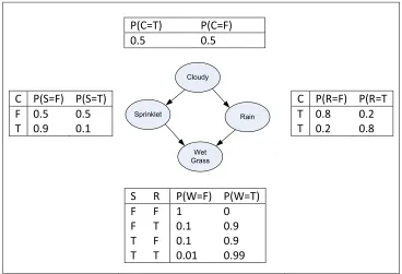
either by rain or by sprinkler. In this example all the variables are binary and the value of the CPTs can also specify the strengths of dependencies. The network presented in Figure 2.1 encodes the following joint probability distribution.
) , | ( ) | ( ) | ( ) ( ) , , ,
(C R S W PC P R C P S C PW R S
P
Figure 2.1 a simple Bayesian network. (Murphy, 2002)
Both the structure and parameters (the set of all CPTs) can be learned from data. The major challenge in using Bayesian networks is learning their structure. Based on the nature of the modeling, structure learning methods are classified in two groups: constrained-based and score-and-search (Larrañaga & Lozano, 2002). The first group tries to discover the structure by finding the independency relations among subsets of variables and gives as an output a DAG (Heckerman, 1999). The second group uses some scoring functions to measure the quality of every candidate network. In fact, the scoring
P(C=T) P(C=F)
0.5 0.5
C P(S=F) P(S=T) F 0.5 0.5 T 0.9 0.1
Wet Grass Cloudy
Rain Sprinklet
C P(R=F) P(R=T T 0.8 0.2 T 0.2 0.8
S R P(W=F) P(W=T)
F F 1 0
F T 0.1 0.9
T F 0.1 0.9
function measures the fit of the network to the data. A search algorithm is used to explore the space of the possible networks and find the network with highest score. Since the number of networks is super-exponential in number of variables, heuristic search algorithms are used, such as different versions of greedy hill climbing with multiple start points or tabu Search (Glover & Laguna, 1993), (Glover & Laguna, 1993), simulated annealing (Bouckaert, 1995) or MCMC (York & Madigan, 1995), and some stochastic population-based search algorithms such as genetic algorithms (Larrañaga, et al., 1996). Scoring functions are based on different principles, such as Bayesian approach (Cooper & Heskovits, 1992), (Heckerman, et al., 1995), entropy (Herskovits, et al., 1990), and Minimum Description length (MDL) (Lam & Bacchus, 1994). A comparison between different scores can be found in (Yang & Chang, 2002). The two most popular scores are Bayesian Score and BIC/MDL Score. Bayesian Score is the logarithm marginal likelihood of the parameters. In this chapter we used two Bayesian Scores: BDeu Score (Heckerman, et al., 1995), and K2 score (Cooper & Heskovits, 1992) and we refer to the latter as Bayes score. The difference between these two scores is in the choices on priors on count. BIC/MDL is defined as the logarithm of probability of data knowing marginal likelihood of parameters plus a penalty term. These metrics are decomposable which means that the score of a network is equal to the sum of the scores of its nodes.
2.3 Search Heuristics
The most straightforward method for learning Bayesian networks is using a simple hill climbing heuristic. Starting from an empty or random network, all the possible moves (adding, deleting, and reversing an edge) are considered and the one that improves the score of the network the most is chosen at each step. The repeated version of this algorithm is used for escaping from local optimum. It restarts the search from randomly generated networks and returns the network with the highest score in various independent runs.
Tabu Search is another hill climbing algorithm. This algorithm continues the search after reaching a local optimum by choosing a move that makes the least reduction in the score of the network. A list of recently performed operations is kept and they are not considered to prevent a cycle of repetitive operations. Tabu search algorithm returns the best network visited during the traverse of the search space.
One way to improve the efficiency of hill climbing method is to use a look ahead hill climbing algorithm, for example LAGD (Holland, et al., 2008). This algorithm considers a sequence of best moves instead of considering the best move at each step. Since it is very time consuming to find the best sequence among all the possible moves, it first finds a set of good moves and then finds the best sequence of moves among them.
Specifying an order on the variablesVi makes it possible to learn the network very efficiently. If
i
V precedes Vj in an ordering, no structure with an edge form Vj to
should be done (Luis & Puetra, 2001), (Witten & Frank, 2000). A score should be assigned to each possible order and local moves should be defined. The swapping of two variables in the order can be an example of local move in the space of orders. The score of the best network consistent with an order is usually considered as the score of the order. Any version of hill climbing, such as tabu search, can be used to find the best score. After finding the score of the order, the best network can be found using K2 algorithm. It is also possible to just repeat K2 algorithm with random orders and keep the best result (Repeated K2).
Another search heuristic that is used for learning Bayesian networks is simulated annealing (Bouckaert, 1995). In this method, a candidate network is generated by randomly adding or deleting or reversing an edge. If the score of this network is better than the current one, it is accepted otherwise it is accepted with the probability
) exp(
T Q
P . Where Q and T are the change in the quality of the network and the current temperature. As the temperature of the system decreases, the probability of accepting a worse move is decreased. If the temperature goes toward zero, then only better moves will be accepted.
2.4 Experiments
2.4.1 Problem Definition
number of evaluations needed by the slowest algorithm, LAGD, to complete its search. We have studied the effects of the size of the networks, of the scoring functions, of the size of datasets and of the algorithms parameters on the accuracy of the learned networks.
2.4.2 Networks and Datasets
The datasets used in our experiments are generated from random networks with various numbers of variables. The numbers of variables (nodes) in the networks we have considered are 10, 20, 30, 50, 70 and 100. For each network size, we generated 10 random networks. From each of these networks, we generated one small datasets with at least 1000 records. We call each record an instance. We found out that increasing the number of instances to more than 10000 does not improve the performance metrics significantly. Therefore we sampled 10000 instances from the networks for our large datasets. In total, we have carried out our experiments for 60 networks, 10 for each size, and presented the average of the performance metrics for each size of networks and datasets. Table 2.1 shows the characteristic of networks and data sets we used in our experiments and also the average number of network evaluations that have been performed for each of them. The networks are classified into three groups based on their size.
2.4.3 Performance Metrics
The following performance metrics have been measured in the experiments.
Divergence between the probability distribution represented by the true networks and the learned networks. It is equal to ( )log ( )/ ( )
1 i i
m i i i X Q X P X P
. } ,..., 1{X 1 Xm
X } is a set of instances andP(Xi) and Q(Xi) are the probabilities of the two networks for the instance Xi. Each instance is a set of
values for n variables.
The values of Bayes, BDeu, and MDL scores for the learned networks.
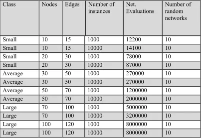
Table 2.1 Networks used in the experiments.
Class Nodes Edges Number of instances Net. Evaluations Number of random networks
Small 10 15 1000 12200 10
Small 10 15 10000 14100 10
Small 20 30 1000 78000 10
Small 20 30 10000 87000 10 Average 30 50 1000 270000 10 Average 30 50 10000 270000 10 Average 50 70 1000 1200000 10 Average 50 70 10000 2000000 10 Large 70 100 1000 5000000 10 Large 70 100 10000 3200000 10 Large 100 120 1000 8000000 10 Large 100 120 10000 8000000 10
Repeated Hill Climber (RHC), tabu search, LAGD and Simulated annealing (SA). We also added an order based search (OBS) to the existing algorithms and used a repeated version of K2 (RK2). In all of these algorithms the maximum number of network evaluations and the maximum number of parents allowed for each node are limited to 5 nodes.
2.5 Results
2.5.1 Small Data Sets
Tables 2.2, 2.3 and 2.4 present the average of different performance metrics for each of the learning algorithms using small datasets. They correspond to the results for respectively small, average and large networks. The results in each table are the average of 10 runs on data generated from different random networks. Divergence is the average of the absolute values of the divergence between each learned network and the true network.
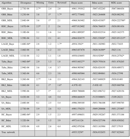
Table 2.2 Small data set result part 1: Average of performance measures using data
set of 1000 instances generated from 10 random networks with 10 nodes and 15
edges. The top three values for each performance metrics are marked with a star.
Algorithm Divergence Missing arcs
Extra
arcs
Reversed
arcs
Bayes score Bdeu score MDL score
OBS_Bayes 2.73E-04 2.7* 2.4 2.8 -4961.191012 -5047.452245 -5047.066436
OBS_Bdeu 3.23E-04 3.8 1* 1.7* -4972.775692 -5023.264608 -5028.002592
OBS_MDL 2.84E-04 3.6 1* 2.1 -4968.563482 -5020.43385* -5024.222788*
RHC_Bayes 3.87E-04 2.3* 2 2.6 -4957.012402 -5036.766019 -5038.081436
RHC_Bdeu 3.10E-04 3.1 1.6 3.4 -4961.009207 -5020.832514 -5025.162375
RHC_MDL 3.59E-04 3.1 2.1 4.1 -4964.824375 -5021.53828* -5025.051215*
LAGD_Baye 1.60E-04* 2.8 1.2 1.7* -4954.3563* -5031.102983 -5032.73435
LAGD_Bdeu 3.46E-04 3.4 1.2 3.5 -4965.037478 -5020.56309* -5025.116
LAGD_MDL 3.51E-04 3.2 1.1 1.8 -4958.634693 -5014.9298* -5018.25762*
Tabu_Baye 1.96E-04* 2.9 1.3 1.8 -4955.84327* -5029.793616 -5031.876265
Tabu_Bdeu 2.94E-04 3.6 1.4 3.7 -4964.905967 -5026.024195 -5030.409371
Tabu_MDL 3.36E-04 4.6 2.3 3.8 -4980.045044 -5032.004861 -5036.27598
RK2_Bayes 3.26E-04 2.7* 1.6 2.3 -4964.262143 -5037.048829 -5038.01401
RK2_Bdeu 5.06E-04 4.1 1* 1.6* -4.97E+03 -5.03E+03 -5029.868704
RK2_MDL 3.99E-04 3.7 1* 2.2 -4969.700688 -5023.896712 -5027.620156
SA_Bayes 4.43E-04 3.3 4.8 5.4 -4984.666819 -5119.940051 -5109.28221
SA_Bdeu 2.68E-04 4.1 2.5 5.4 -4986.589105 -5053.786108 -5057.998785
SA_MDL 2.73E-04 3.9 2.6 5.3 -4981.576233 -5049.288606 -5051.253407
HC_Bayes 2.00E-04* 2.9 1.5 2.3 -4957.694651 -5029.192267 -5031.571184
HC_Bdeu 3.32E-04 3.9 1.5 3.9 -4973.61124 -5034.527196 -5038.850262
HC_MDL 3.85E-04 4.8 2.6 4.4 -4982.070246 -5033.163984 -5037.37919
We could not find any rule that shows using which algorithm or score is better for having the minimum divergence. In some experiments the algorithm which on average learned the network with least divergence shows the worst performance for other measures. In more than 80 percent of the experiments LAGD and tabu algorithms with Bayes score could find networks with least number of missing edges and also least number of reversed edges. But in most cases there are other algorithms that find the network with less extra edges. If we consider the sum of missing edges and extra edges as a performance measure we can see that LAGD with MDL score outperforms other algorithms. LAGD with other scores also gives good results. LAGD and tabu with Bayes scores usually shows the least number of reversed edges and each algorithm has the most extra edges when we use it with Bayes score.
In all of these algorithms we try to optimize the score of the networks, so we expect that the score of the true network is the highest. But we see that only with small datasets the true network has the highest Bayesian score and it does not have the best BDeu or MDL score even when we use these scores in our search algorithms.
Since datasets are small, they do not contain enough instances to represent the distribution of the data set accurately, so other networks might fit the dataset better than the true networks. LAGD and tabu with MDL are most of the time among the top three algorithms that gives us best MDL and BDeu scores.
Table 2.3 Small data set result part 2: Average of performance measures using data
set of 1000 instances generated from 10 random networks with 30 nodes and 50
edges. The top three values for each performance metrics are marked with a star.
Algorithm Divergence
Missing
arcs
Extra
arcs
Reversed
arcs Bayes score Bdeu score MDL score
OBS_Bayes 1.28E-09 9.2 13 10.1 -15403.08317 -15756.74477 -15729.7251
OBS_Bdeu 1.14E-09 13 8 11.3 -15427.19138 -15634.8109 -15628.7074
OBS_MDL 1.86E-09 11.7 5.9 9.1 -15396.302 -15620.62708 -15603.743
RHC_Bayes 1.40E-09 5.9* 12 8.2 -15305.39625 -15656.41101 -15636.93364
RHC_Bdeu 1.24E-09 10 6.1 7.3 -15350.49382 -15562.50049 -15556.6421
RHC_MDL 1.23E-09 9.5 5.8 8.9 -15338.17658 -15555.08157 -15540.40124
LAGD_Baye 1.60E-09 6* 9.7 4.5* -15292.053* -15628.69071 -15613.73211
LAGD_Bdeu 9.17E-10 9.4 4.9* 7.2 -15320.2306 -15537.66102 -15530.37685
LAGD_MDL 1.13E-09 9.1 5.1* 7.7 -15314.41803 -15531.389* -15517.256*
Tabu_Bayes 1.50E-09 6.3* 9.3 4.8* -15294.3848* -15623.92899 -15609.21109
Tabu_Bdeu 9.03E-10 10.4 5.9 7.7 -15344.90897 -15552.5953* -15548.34053*
Tabu_MDL 1.15E-09 9.4 5.4* 8.1 -15324.29737 -15537.4343* -15524.71807*
RK2_Bayes 1.57E-09 8.9 13.2 11 -15389.79182 -15736.48206 -15716.00844
RK2_Bdeu 1.47E-09 13.3 6 9.8 -1.54E+04 -1.56E+04 -15627.81419
RK2_MDL 1.33E-09 12.4 6.6 9.5 -15423.45253 -15637.34985 -15623.05819
SA_Bayes 2.54E-09 10.7 26.3 17.7 -15638.47792 -16138.19466 -16087.31551
SA_Bdeu 6.73E-10* 14.4 14.6 14.2 -15528.07226 -15779.81795 -15767.3898
SA_MDL 7.13E-11* 13 13.5 17.1 -15525.86118 -15776.25718 -15757.05586
HC_Bayes 1.54E-09 6.4 9.2 6.1* -15298.02631 -15632.36313 -15617.07862
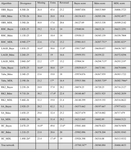
Table 2.4 Small data set results part 3: Average of performance measures using data
set of 1000 instances generated from 10 random networks with 70 nodes and 100
edges. The top three values for each performance metrics are marked with a star.
Algorithm Divergence Missing arcs
Extra
arcs
Reversed
arcs
Bayes score Bdeu score MDL score
OBS_Bayes 8.50E-26 26.4 45.6 23.2 -36087.036 -36815.969 -36806.3723
OBS_Bdeu 8.75E-26 30.6 20.8 19.8 -36154.415 -36585.196 -36592.4977
OBS_MDL 3.38E-26 30.8 17.6 20.6 -36127.69 -36513.338 -36509.2142
RHC_Bayes 1.82E-25 19.2 51.4 14 -35840.84 -36632.24 -36633.3291
RHC_Bdeu 1.13E-25 22.4 18.4 14 -35930.13 -36345.159 -36358.7804
RHC_MDL 4.94E-27* 22.6 17.6 15.2 -35901.015 -36307.751* -36301.823*
LAGD_Baye 1.83E-25 16.6* 50.6 11.8* -35817.84* -36630.657 -36636.7457
LAGD_Bdeu 2.26E-25 23.2 19 16.6 -35959.551 -36359.22 -36372.8294
LAGD_MDL 2.06E-26* 22.2 17* 15.2 -35904.54 -36294.715* -36293.219*
Tabu_Bayes 2.67E-25 16.6* 50.8 13* -35839.011* -36673.981 -36679.0496
Tabu_Bdeu 2.34E-25 23.6 19.8 18 -35974.076 -36367.959 -36383.1722
Tabu_MDL 2.19E-26 23.2 17* 16.4 -35915.586 -36303.729* -36302.7966*
RK2_Bayes 2.23E-26 24.8 37.8 20.2 -36074.25 -36720.25 -36716.2127
RK2_Bdeu 9.71E-26 30.2 17.4* 22.4 -36160.467 -36531.925 -36542.2039
RK2_MDL 5.46E-26 32.2 19.8 21.4 -36140.399 -36519.193 -36516.0622
SA_Bayes 2.92E-25 28.2 82.2 31.2 -36373.662 -38197.667 -37977.6321
SA_Bdeu 1.65E-25 29.6 32.4 25.2 -36237.679 -36718.002 -36717.479
SA_MDL 4.88E-26 29 31.4 29.2 -36213.845 -36682.89 -36664.5121
HC_Bayes 2.67E-25 16.8* 49.6 13.6* -35841.444 -36670.423 -36674.9458
HC_Bdeu 1.21E-25 23.8 20.6 20 -35982.096 -36378.204 -36391.9343
HC_MDL 1.49E-26* 23.4 17.4* 19 -35926.398 -36316.08 -36313.9332
2.5.2 Large Data Sets
We repeated the experiments of Section 3.1 with dataset of 10000 instances. The results for the representatives of each of different classes, small, average and large networks, are presented in table 2.6, 2.7 and 2.8.
Table 2.5 Number of times that an algorithm is located in the top three best in table
2.2, 2.3 and 2.4 of the for each performance measure for small data sets.
Algorithm Divergence Missing
edges( M) Extra edges(E) Reversed edges(R) Bayes score Bdeu score
MDLScore Mi+E M+E+R
OBS_Bayes 1 0 0 0 0 0 0 0 0
OBS_Bdeu
OBS_Bdeu
0 0 2 2 0 0 0 0 1
OBS_MDL 3 0 2 0 0 0 1 1 0
RHC_Bayes 1 3 0 0 1 0 0 1 0
RHC_Bdeu 2 0 0 0 0 1 0 0 0
RHC_MDL 1 0 0 0 0 1 4 1 1
LAGD_Baye 1 5 0 6 6 0 0 3 4
LAGD_MDL 2 0 2 0 0 5 6 4 3
Tabu_Bayes 1 5 0 5 4 0 0 1 3
Tabu_Bdeu 0 0 1 0 0 0 0 1 1
Tabu_MDL 0 0 2 0 0 4 5 2 0
RK2_Bayes 0 1 0 0 0 1 0 0 0
RK2_Bdeu 0 0 1 1 0 0 0 0 0
RK2_MDL 0 0 3 0 0 0 0 1 0
SA_Bayes 0 0 0 0 1 0 1 0 0
SA_Bdeu 2 0 0 0 0 0 0 0 0
SA_MDL 1 0 0 0 1 1 0 0 0
HC_Bayes 1 3 0 4 0 0 0 0 0
HC_Bdeu 1 0 1 0 0 0 0 1 0
HC_MDL 1 0 0 0 0 0 0 0 0
Table 2.6Large data set results part1: Average of performance measures using data
set of 10000 instances generated from 10 random networks with 10 nodes and 15
edges. The top three values for each performance metrics are marked with a star.
Algorithm Divergence
Missing
arcs
Extra
arcs
Reversed
arcs Bayes score Bdeu score MDL score
OBS_Bayes 1.97E-04 1.2 6.7 4.1 -49249.03613 -49432.77094 -49419.61083
OBS_Bdeu 1.35E-04 1 2.6 3.6 -49184.33229 -49300.67223 -49299.08134
OBS_MDL 1.32E-04 1 2.9 7.3 -49198.91038 -49307.55883 -49306.42171
RHC_Bayes 3.74E-05* 0.4* 1.3 2.4* -49157.16168* -49241.5274* -49241.28549*
RHC_Bdeu 9.82E-05 0.8 3.2 4.8 -49179.47897 -49274.44183 -49273.34651
RHC_MDL 3.53E+09 0.9 2.9 5.7 -49172.54986 -49258.71706 -49258.7359
LAGD_Baye 3.20E-05* 0.6* 0.7* 1.1* -49153.378* -49238.2693* -49238.6602*
LAGD_Bdeu 4.22E-05 0.8 1.5 3.7 -49161.70999 -49246.76996 -49247.73991
LAGD_MDL 4.12E-05 0.8 1.2* 3.1 -49162.8478 -49248.852 -49249.533
Tabu_Bayes 3.16E-05* 0.6* 1.2* 2.2* -49158.15139 -49243.77858 -49245.00887
Tabu_Bdeu 5.01E-05 1.1 2.4 4.3 -49187.67735 -49275.26233 -49275.41128
Tabu_MDL 1.48E-04 1 2.4 5.1 -49228.04419 -49316.09981 -49314.84195
RK2_Bayes 3.87E-05 0.5* 1.7 2.7 -49162.73292 -49252.94241 -49253.40994
RK2_Bdeu 1.14E-04 0.7 1.9 3.1 -4.92E+04 -4.93E+04 -49260.43787
RK2_MDL 4.68E-05 0.6 1.1* 2.5 -49158.91522 -49245.67045 -49245.84179
SA_Bayes 6.92E-04 1.8 8.8 6.6 -50066.84477 -50251.86098 -50238.88191
SA_Bdeu 6.67E-04 2.1 7.6 7.1 -50053.72464 -50206.82733 -50193.83396
SA_MDL 6.98E-04 1.8 7.4 7.1 -49925.68533 -50082.19628 -50069.68936
HC_Bayes 3.76E-05 0.6 1.6 3 -49165.55376 -49259.21916 -49259.37932
HC_Bdeu 9.46E-05 1.2 3 5.2 -49200.27206 -49300.35981 -49301.05191
HC_MDL 1.55E-04 1.3 3.1 6.7 -49310.20744 -49401.02595 -49399.68765
Table 2.7 Large data set results part1: Average of performance measures using data
set of 10000 instances generated from 10 random networks with 30 nodes and 50
edges. The top three values for each performance metrics are marked with a star.
Algorithm Divergence
Missing
arcs
Extra
arcs
Reversed
arcs Bayes score Bdeu score MDL score OBS_Bayes 1.32E-09 3.6 17.9 14.4 -150915.93 -151413.4 -151358.73
OBS_Bdeu 1.71E-09 4.6 15.5 12.6 -150802.94 -151221.58 -151179.21
OBS_MDL 7.08E-10 5 16 13.8 -150984.3 -151437.28 -151380.54
RHC_Bayes 4.74E-10 2.7 14.2 11.6 -150601.98 -151021.81 -150983.1
RHC_Bdeu 6.14E-10 2.7 10.1 9.9 -150552.13 -150913.34 -150882.42
RHC_MDL 5.53E-10 3.5 13.1 13.2 -150685.52 -151067.44 -151027.72
LAGD_Bayes 8.69E-11* 1.5* 3.9* 4.7* -150394.35* -150719.03* -150702.52*
LAGD_Bdeu 3.29E-10 1.9* 2.3* 4.6* -150431.88 -150738.18 -150721.36
LAGD_MDL 4.10E-11* 2.3 3.2* 5.9 -150313.75* -150621.22* -150599.44*
Tabu_Bayes 2.19E-10 1.9* 4.9 5.7* -150458.25 -150787.96 -150769.5
Tabu_Bdeu 3.22E-10 2.4 3.9* 5.9 -150433.34 -150741.56 -150725.37
Tabu_MDL 3.22E-10 3.1 5.5 8.6 -150443.52 -150759.94 -150732.73
RK2_Bayes 1.66E-09 5.4 21.1 16.2 -151084.3 -151612.07 -151549.42
RK2_Bdeu 1.64E-09 5.5 16 13.3 -151104.11 -151549.85 -151504.76
RK2_MDL 1.02E-09 4.9 18.4 14.9 -151015.14 -151494 -151433.33
SA_Bayes 4.45E-09 10.4 36.9 19.8 -156656.57 -157356.71 -157240.2
SA_Bdeu 1.27E-09 9.4 33.1 19.6 -156057.1 -156679.95 -156579.72
SA_MDL 5.34E-09 10 33.5 18.7 -155967.21 -156597.81 -156490.04
HC_Bayes 2.61E-10* 2.1 5.9 6.8 -150478.9 -150817.22 -150796.35
HC_Bdeu 3.39E-10 2.9 5.6 7.9 -150486.61 -150803.4 -150785.36
HC_MDL 2.18E-10 3.5 7.2 10 -150561.26 -150884.95 -150857.85
Table 2.8 Large data set results part 3: Average of performance measures using
data set of 10000 instances generated from 10 random networks with 70 nodes and
100 edges. The top three values for each performance metrics are marked with a
star.
Algorithm Divergence Missing arcs
Extra
arcs
Reversed
arcs
Bayes score Bdeu score MDL score
OBS_Bayes 2.20E-24 11.33 43.33 36.67 -356070.306 -357053.6672 -356942.0786
OBS_Bdeu 1.25E-24 11.67 44.33 30 -355844.704 -356795.9116 -356691.7556
OBS_MDL 1.37E-24 12 37 28 -355615.349 -356475.12 -356387.3466
RHC_Bayes 1.22E-25* 6.33 30.67 20.33 -354383.903 -355211.3996 -355129.9116
RHC_Bdeu 8.38E-25 6.33 31.33 24.67 -354273.506 -355051.7284 -354976.8621
RHC_MDL 1.36E-24 7 29.67 24.67 -354320.996 -355073.517 -355005.7985
LAGD_Baye 3.19E-25* 5.33* 21 15.33* -354005.022* -354727.1159* -354669.452*
LAGD_Bdeu 6.56E-25 6* 15.33* 15.33* -354063.237 -354740.859 -354686.497
LAGD_MDL 2.16E-25* 5.67* 10* 12.67* -353858.842* -354492.4059* -354449.216*
Tabu_Bayes 7.77E-25 6* 22 16.67 -354122.87 -354838.2077 -354781.6592
Tabu_Bdeu 5.60E-25 6.33 19.33 19 -354130.489 -354828.712 -354773.3761
Tabu_MDL 1.03E-24 8 18.67* 18.67 -354145.743 -354808.5963 -354760.97
RK2_Bayes 1.41E-24 10.67 41.33 28.33 -355744.165 -356615.376 -356529.1746
RK2_Bdeu 1.32E-24 9.33 33 29 -355377.281 -356158.6645 -356087.1745
RK2_MDL 1.70E-24 12.33 42.33 35 -355887.874 -356743.2825 -356665.3144
SA_Bayes 5.54E-24 19 90.33 37.33 -361813.344 -365434.1678 -364675.0585
SA_Bdeu 9.38E-25 18.33 67.67 41.67 -360269.49 -361828.1383 -361565.3648
SA_MDL 4.87E-24 21.33 78.33 40 -361621.022 -363471.7872 -363128.0832
HC_Bayes 7.77E-25 6 22.33 17 -354123.721 -354839.6313 -354782.8973
HC_Bdeu 1.11E-24 6.67 22.67 26.33 -354194.054 -354923.5783 -354862.9895
HC_MDL 1.05E-24 8.33 20 23 -354158.23 -354824.7936 -354778.8307
Table 2.9 Number of times that an algorithm is located in the top three in Tables
2.6, 2.7 and 2.8 for each performance measure for large dataset.
Algorithm divergence
Missing edges(M)
Extra edges(E)
Reversed edges(R)
Bayes score
Bdeu
score MDLScore Mi+E M+E+R
OBS_Bayes 0 0 0 0 0 0 0 0 0
OBS_Bdeu 0 0 0 0 0 0 0 0 0
OBS_MDL 1 0 0 0 0 0 0 0 0
RHC_Bayes 1 4 0 1 1 1 1 1 1
RHC_Bdeu 2 1 0 0 2 1 0 0 0
RHC_MDL 1 0 0 0 0 0 0 1 0
LAGD_Baye 3 5 5 6 5 5 4 4 6
LAGD_Bdeu 1 2 4 4 0 0 0 4 4
LAGD_MDL 3 1 5 3 2 4 4 4 5
Tabu_Bayes 1 3 0 1 2 0 0 0 2
Tabu_Bdeu 1 0 1 0 1 1 1 2 0
Tabu_MDL 0 0 2 0 0 0 0 1 0
RK2_Bayes 0 1 0 0 0 0 0 0 0
RK2_Bdeu 1 0 0 0 0 0 0 0 0
RK2_MDL 0 0 0 0 0 0 0 1 0
SA_Bayes 0 0 0 0 0 0 0 0 0
SA_Bdeu 0 0 0 0 0 0 0 0 0
SA_MDL 0 0 0 0 0 0 0 0 0
HC_Bayes 0 0 0 0 0 0 0 0 0
HC_Bdeu 0 0 0 0 0 0 0 0 0
HC_MDL 2 0 0 0 0 0 0 0 0
As we increase the size of datasets we can see more consistency in the results. Although there is not any single algorithm that gives us the least divergence, LAGD with Bayes or MDL scores ranked among the top three of each table in 83 percent of the experiments. We can also see that the true network has the highest score no matter what score we use as performance measure. For small networks LAGD and repeated hill climbing with Bayes score could find the networks with the highest scores and the least missing arcs. For large and average size networks, LAGD with different scores has the best overall performances followed by tabu search that performs quite well and can find networks with high scores. Table 2.9 shows that LAGD with different scores gives the least number of extra and reversed edges. Actually it seems that when we have sufficient data, what is more important is the algorithm and all scores are almost equivalent. With sufficient data simulated annealing always has the worst results no matter which score we use.
2.6 Conclusion
one algorithm does not necessarily indicate that algorithm works that well for other networks even with the same size and in many cases another algorithm performs better. Therefore it makes the performance of many algorithms tested just questionable for some small benchmark networks. We found that in many cases, having the highest quality score does not mean that there is a least divergence between the distribution presented by true network and the learned network. Hence we cannot conclude that the network with high quality always perform better for a specific application. Actually this result is similar to what presented in (Acid & Campos, 2004) which shows that the network with highest score, learned from a medical emergency dataset of 11 variables, is not the best one when it used for some predictions.
In the case of PMBGA, our goal is finding the network that represents the dependencies of variables the best. Therefore the least number of missing and extra arcs are desirable. As we can see in tables 2.5 and 2.9, LAGD algorithm in most cases finds the networks with these characteristics, no matter which score and what size of datasets are used. This algorithm is also faster comparing the other algorithm with the same number of network evaluations.
Chapter 3
Estimation of Distribution of Algorithms
In this chapter we first describe GA, the ancestor of EDA and explain the motivation behind emergence of EDA as an alternative of GA. Then we present a survey of EDAs with more emphasis on discrete EDAs. We follow (Pelikan, 2005) and categorize these EDAs based on the order of interaction between variables taken into account by probabilistic models used in these EDAs. Finally we present a survey of application of EDA in gene expression data analysis.
3.1 Genetic Algorithms
form of a function f(x) known as fitness function. For example, a function which simply returns the sum of 1s in a bit-string, known as OneMax function in literature (Mühlenbein & Paaß, 1996), is presented in Figure 3.1.
The set of all possible solutions is known as the search space. For the 5 bit long chromosome shown in Figure 3.1, the search space consists of 32 solutions.
A solution (chromosome) fitness
3 ) ( 1
n i i i x x f1 0 1 1 0
}
,
,
,
,
{
x
1x
2x
3x
4x
5x
Figure 3.1 A solution and its fitness for 5 bit OneMax
Figure 3.2 Genetic algorithm pseudo-code. Genetic Algorithm
1. Generate initial population of solutions P of size M (initialization ) 2. Select N promising solutions from parent population P, where
N≤ M (selection)
3. Perform crossovers and mutations on the selected population also known as breeding pool to get a new population which is also known as child population (variation)
The GA starts by initialising a population of solutions known as the parent population. The main iteration then starts by performing selection, crossover and mutation operations, and forms a child population that replaces the parent population. This process is then iterated until some termination criteria are satisfied.
Figure 3.2 presents the pseudo-code of a simple GA. Generation of initial set of solution (initial population) P is done usually randomly according to a uniform distribution of possible solutions in the search space. However, it is also possible to use the output solutions of another search algorithm as the initial population. Sometimes, the initial population is seeded with solutions that are not random.
Different selection methods can be used depending on the design of the algorithm in order to select a subset the promising solutions. These methods can be categorised into two groups: proportional selection and ordinal selection.
In proportional selection, first, the selection probability for each individual in the current population is determined, and then the new set of solutions is sampled using these probabilities. The fitness proportionate selection (also known as Roulette wheel selection) (Goldberg, 1989)) and Boltzmann selection (De la Maza & de la Maza, 1993) falls in this category. In fitness proportionate selection, the selection probability Ps(x) for a solution x is determined as
S y s y f x f x P ) ( ) ( ) ( .In Boltzmann selection, the selection probabilityPs(x) for a solution x is determined as
f fx yTT
s
e e x
Where, T is a parameter for the selection known as temperature.
In ordinal selection, the selection probability is not calculated from the numerical value of the fitness function. Instead the selection decision is based on the ranked order of fitness values. Some of the popular ordinal selection methods include tournament selection, and truncation selection (Goldberg, 1989), (Mitchell, et al., 1994) and (Harik, 1999). In a typical tournament selection, the fittest out of two (or more) randomly chosen chromosomes from parent population is selected. In truncation selection, the N fittest solutions from the parent population are selected at once. However, the general motive behind all selection methods is the same, namely to provide a selection pressure in favour of better solutions. As such, the selection process models the idea of survival of the fittest individuals.
same positions between the selected solutions. Figure 3.3 presents an example of one-point crossover.
1 0 0 1 1 1 0 1 0 0 1 0 1 1
0 0 1 1 0 1 1 0 0 1 1 1 1 0
Figure 3.3 An example of one-point crossover.
Another source of variation in GA is the mutation operator. Exploring those parts of search space which is not possible with crossover operator (if a particular value for a variable is not present in the initial population for example) is feasible with mutation operator. This operator changes some part of a solution into some other possible value and is similar to the random genetic variation between parents and offspring. The probability of mutation also is a parameter of GA which should be predefined. This probability is usually very small. Therefore the crossover operator is the major source of variation in GAs. These GAs are also known as selectorecombinative in literature (Pelikan, 2005) . An example of single bit mutation in a 7 bit solution is presented in Figure 3.4.
Before mutation
0 0 1 1 0 1 1 0 0 1 1 1 1 1
As we can see in the GA algorithm (Figure 3.2), after applying the crossover operator and the mutation operator on the promising solutions, the original solutions are replaced by new ones. This new set of solutions is used in the next iteration of the algorithm unless some termination criteria are met. For example when the algorithm reaches the upper bound on the number of generations, the population converges to a unique solution or simply a good enough solution is found in the population.
3.1.1 GA limitations
and Fast Messy Genetic Algorithm (fmGA) (Kargupta, 1998). In these algorithms, first the important building blocks are specified by using the selection operator and other parts of solution are substituted by a template solution which itself is updated every few generations. Then selection and crossover operators are used to mix these important building blocks. Another algorithm in the first class is Linkage Learning Genetic Algorithm (LLGA) (Harik, 1999). LLGA maps the variables of the problem onto a circle. The mutual distances between these variables evolve gradually during optimization process and therefore it is less likely that crossover operator disrupt them.
The second class of algorithms solves the linkage problem by changing the principle of recombination and using new ways for generating variation. These algorithms generate new solutions by using information extracted from the set of promising solutions. This information can be used to estimate the distribution of promising solutions and subsequently this estimate can be used to generate a new set of solutions. These kinds of algorithms are called Estimation of Distribution Algorithms (EDAs). Estimating the distribution can be a difficult task and there is a trade-off between the accuracy and computational time. Besides Linkage problem, choosing various parameters including crossover and mutation probabilities also have been among the motives for the emergence of the EDAs.
3.1.2 An Alternative for Generating Variation
A simple alternative for crossover operation can be obtained by calculating the frequency of having 1s in each positions of all the promising solutions and computing the probability p(Xi 1) of having one for that position. Then, the new candidate solutions are generated by setting in each solution the bit at position i to 1 with probability
) 1 (Xi
p and to 0 with probability 1- p(Xi 1). This method for generating new solutions is also known as probabilistic uniform crossover in literature (Pelikan, 2005). Although with this kind of recombination all the variables are considered independent and, therefore, it is not able to solve the linkage problem, we use it to show how it is possible to generate variations without crossover and mutation. Actually this algorithm can work better than simple genetic algorithm for problems with independent variables converging to the global optimum faster.
3.2 Estimation of Distribution Algorithms
probability vector which is updated in each generation based on the fittest individuals and using a mutation operator. Numerous variations of EDAs have been introduced up to now. Most of these algorithms are designed to solve discrete problems and the solutions are represented as binary vectors. Although several EDAs have been proposed for solving problems with continuous and mixed variables as well (Bosman & Thierens, 2000), (Larrañaga & Lozano, 2002), in this chapter we focus on the discrete domain and introduce main classes of EDAs. The steps of an EDA are summarized in the algorithm presented in Figure 3.6 and Figure 3.7.
Figure 3.6 EDA pseudo-codes
In addition to guiding through the search space, the probabilistic models learned in EDAs can represent a priori information about the problem structure. This information can be used for a more efficient search of optimum solutions. In case of Black box optimization
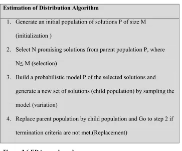
Estimation of Distribution Algorithm
1. Generate an initial population of solutions P of size M (initialization )
2. Select N promising solutions from parent population P, where N≤ M (selection)
3. Build a probabilistic model P of the selected solutions and
generate a new set of solutions (child population) by sampling the model (variation)
problems (where the objective function is modeled as a black box) the probabilistic model can reveal important unknown information about the structure of the problems (Pelikan, et al., 2001). The probabilistic models learned during the execution of the algorithm can also be considered as models of the function to be optimized and therefore might be used for predicting the values of the function when the function is unknown. The main difference between different EDAs is due to the class of probabilistic models they use, although the different selection and replacement strategies used in them can also have significant effects in their efficiency. Choosing the best EDA for a specific problem can be difficult when the structure of the problem is unknown and it might be useful to try different probabilistic models and selection and replacement methods to find the best combination of them for a given problem (Santana, et al., 2008). In the next section we discuss several probabilistic models usually used in EDAs.
3.2.1 Model Building in EDAs
building-model grows exponentially with the size of the building blocks. Therefore a trade-off between the efficiency and accuracy of the method need to be found. The EDAs usually are classified based on the complexity of the probabilistic models used in them. In some models the variables are considered independent or only pair-wise dependencies are considered. However there are EDAs with more complex models which are able to model problems with very complex structure with overlapping multivariate building blocks. In Figure 3.7 different kinds of dependencies among the variables are presented.
(a) no dependency (b) pairwise dependencies (c) multiple depenencies
Figure 3.7 Different kinds of dependencies among variables of a problem.
3.2 .2 Notations
In this section, we adopted the notion used in (Larrañaga & Lozano, 2002). Let Xibe a random variable, and xi be one of its possible values. We use (Xi xi)(or simply
) (xi
) to present the generalized probability density function (gpdf) over the point xi.
Now let X {X1,X2,...,Xn} be a vector of n random variables, and x{x1,x2,...,xn} be a vector of values taken by each variables of the vectorX , (X x)(or simply
) | (xi xj
Let XS be a sub-vector of X and xS be a possible set of values taken byXS, then )
(XS xS
p (or simplyp(xS)) is the marginal distribution of the setXS. Note that univariate marginal distribution is a simple case of marginal distribution, where sub-vector consists of a single variable.
) ( ) , ( ) | ( B B A B A x p x x p x x p
Here, p(xA,xB)is the joint probability distribution (jpd) of the subsets XA xA and B
B x
X .
The factorization of the jpd p(x), then follows
) ( ) | ( )... ,..., | ( ) ,..., | ( )
(x p x1 x2 xn p x2 x3 xn p xn 1 xn p xn
p
The notations represent each search point/individual in a population by a fixed-length vector X (X1,X2,...,Xn) where Xi (i0,...,n) is a random variable for a problem
with n variables. Usually Xi is a binary variable but it can also gets its value from a finite discrete set or even takes a real value. Let x(x1,x2,...,xn) be an instantiation of the vector X. Then P(Xi xi), or simplyP(Xi), is the univariate marginal distribution of the variable Xi and P(x x), orP(x), is the joint probability distribution function of x.
) |
(Xi xi Xj xj
3.2.3 Discrete EDAs
The discrete EDAs use fixed-length strings of finite cardinality to present solutions of a problem. These EDAs can be categorized in three groups based on the order of interaction between the variables: univariate, bivariate and multivariate.
Models with independent variables (univariate EDA)
Assuming that all the variables in a problem are independent it is possible to model them simply by considering a set of frequencies of all values of each variable in the selected set of individuals. In this case, all the variables are considered as univariate and the joint probability distribution is the product of marginal probabilities of the n variables.
) ( ),..., (
) ( ) ,..., ,
(X1 X2 Xn p X1 p X2 p Xn
p
Where p(Xi) is the probability of variableXi, and p(X1,X2,...,Xn) is the probability of
the candidate solution (X1,X2,...,Xn). The univariate model for n variables thus consists of n probability tables and each of these tables defines the probabilities of the different values of the corresponding variable. Since the probabilities of the different values of a variable must sum to 1, one of the probabilities maybe omitted for each variable.
Population Based Incremental Learning (PBIL) (Baluja & Caruana, 1995), (Baluja & Davies, 1997), Univariate Marginal Distribution Algorithm (UMDA) (Mühlenbein, 1998), and compact Genetic Algorithm (cGA) (Harik, et al., 1998) consider no interaction among variables.
(IUMDA) (Mühlenbein, 1998), use a probability vector (p1,p2,...,pn)as the model for generating the new solution. pi denotes the probability of having the value 1 for the variable i. The initial value for each pi is 0.5. The algorithm updates the probability
vector based on the best solution of the selected promising solutions using ,
where (0,1) is the learning rate andxi is the value of ith variable.
cGA also models the population by a probability vector. However, the probability vector modification is performed in a way that a direct correspondence between this vector and the population represented by this vector exists. Like PBIL, each entry pi in the
probability vector is initialized to 0.5. cGA use a variant of binary tournament in which the worst of the two solutions is replaced by the best one to update the probability vector using a population of size N. Ifbi and wi represents the ith position of the best and the
worst of the two solutions then the probability vector update is as follows:
Unlike cGA and PBIL, UMDA selects a population of promising solutions similarly to traditional GAs. Then the frequencies of the values of each variable in the selected set are used to generate new solutions that replace the old ones and this process repeated until the termination criteria are met.
All of these algorithms that do not consider interdependencies of variables are not able to solve the problems with strong dependencies among their variables. However, they are
) ( i i
i
i p x p
p
N w b p
they are widely used in many applications especially in problems with large number of variables such as bioinformatics problems.
Models with pair wise dependencies
To encode the pair wise dependencies between the variables of a problem several probabilistic models have been used. They use a chain, a tree or a forest as a model for representing the interdependencies among variables (Pelikan & Muhlenbein, 1999), (De Bonet, et al., 1997) and (Baluja & Davies, 1997) .
One of the algorithms which have been proposed to model the pair-wise interaction between variables is Mutual Information-Maximizing Input Clustering (MIMIC) algorithm (De Bonet, et al., 1997). The graphical model used in MIMIC is a chain structure that maximizes the mutual information of the neighboring variables. To specify this model an ordering of variables, the probability of the first position and the conditional probability of other variables, given their preceding variable in the chain should be specified. It leads to the following joint probability distribution for a given order i1,i2,...,in.
) ( ) | ( )... | ( ) | ( ) ( 1 3 2 2
1 i i i i i n
i x P x x P x x P x
x P x P n n .