self-tracing lazy functional programs.
White Rose Research Online URL for this paper:
http://eprints.whiterose.ac.uk/118203/
Proceedings Paper:
Chitil, Olaf, Faddegon, Maarten and Runciman, Colin orcid.org/0000-0002-0151-3233
(2016) A Lightweight Hat: : simple type-preserving instrumentation for self-tracing lazy
functional programs. In: Proceedings of 28th Symposium on Implementation and
Application of Functional Languages. ASSOC COMPUTING MACHINERY .
[email protected]
https://eprints.whiterose.ac.uk/
Reuse
Items deposited in White Rose Research Online are protected by copyright, with all rights reserved unless
indicated otherwise. They may be downloaded and/or printed for private study, or other acts as permitted by
national copyright laws. The publisher or other rights holders may allow further reproduction and re-use of
the full text version. This is indicated by the licence information on the White Rose Research Online record
for the item.
Takedown
If you consider content in White Rose Research Online to be in breach of UK law, please notify us by
Self-Tracing Lazy Functional Programs
Olaf Chitil
University of KentUnited Kingdom [email protected]
Maarten Faddegon
University of KentUnited Kingdom [email protected]
Colin Runciman
University of YorkUnited Kingdom [email protected]
ABSTRACT
Existing methods for generating a detailed trace of a computation of a lazy functional program are complex. These complications limit the use of tracing in practice. However, such a detailed trace is desirable for understanding and debugging a lazy functional program. Here we present a lightweight method that instruments a program to generate such a trace, namely the augmented redex trail introduced by the Haskell tracer Hat. The new method is a major step towards an omniscient debugger for real-world Haskell programs.
CCS CONCEPTS
•Theory of computation→Operational semantics; •Software and its engineering→Functionality;
KEYWORDS
omniscient debugger, Haskell, Hat, augmented redex trail, lazy evaluation
ACM Reference format:
Olaf Chitil, Maarten Faddegon, and Colin Runciman. 2016. A Lightweight Hat: Simple Type-Preserving Instrumentation for Self-Tracing Lazy Func-tional Programs. InProceedings of Implementation and Application of Func-tional Languages, Leuven, Belgium, August 31-September 2, 2016 (IFL 2016), 14 pages.
DOI: http://dx.doi.org/10.1145/3064899.3064904
1
INTRODUCTION
A detailed trace of a computation is the basis for any so-called omni-scient debugger for a programming language (Zeller 2009). A trace substantially supports the processes of understanding and debug-ging a program. Today’s computers provide gigabytes of volatile and non-volatile memory. Therefore storing a detailed trace of a substantial part of a computation poses no practical problem. The Big Data challenge for computer science is to define a trace struc-ture, generate it and finally make good use of it. The Haskell tracer Hat defines the augmented redex trail (ART) as a trace structure
Permission to make digital or hard copies of all or part of this work for personal or classroom use is granted without fee provided that copies are not made or distributed for profit or commercial advantage and that copies bear this notice and the full citation on the first page. Copyrights for components of this work owned by others than the author(s) must be honored. Abstracting with credit is permitted. To copy otherwise, or republish, to post on servers or to redistribute to lists, requires prior specific permission and/or a fee. Request permissions from [email protected].
IFL 2016, Leuven, Belgium
© 2016 Copyright held by the owner/author(s). Publication rights licensed to ACM. 978-1-4503-4767-9/16/08. . . $15.00
DOI: http://dx.doi.org/10.1145/3064899.3064904
type Recogniser = [Char] -> Maybe [Char]
lit :: Char -> Recogniser lit x [] = Nothing
lit x (y:ys) = if x==y then Just ys else Nothing
(<|>) :: Recogniser -> Recogniser -> Recogniser (rl <|> rr) xs = rl xs `mplus` rr xs
mplus :: Maybe a -> Maybe a -> Maybe a mplus Nothing mr = mr
mplus ml _ = ml
binaryDigit :: Recogniser
binaryDigit = lit '0' <|> lit '1'
main = print (binaryDigit [])
Figure 1: A simple recogniser for words in an LL(1) grammar.
and comprises tools for generating and using it (Section 9). This paper is about a better method for generating the ART.
Consider the Haskell program in Figure 1. A recogniser deter-mines whether a given word is within a given LL(1) grammar. If a prefix of the given word is in the grammar, then a recogniser returnsJust xswithxsbeing the remainder of the input word; otherwise the recogniser returnsNothing. Only the combinators necessary for defining the recogniser of a binary digit, which is0 or1, are given. Computation starts with evaluatingmain, which applies the recogniser to the empty list. The result isNothing.
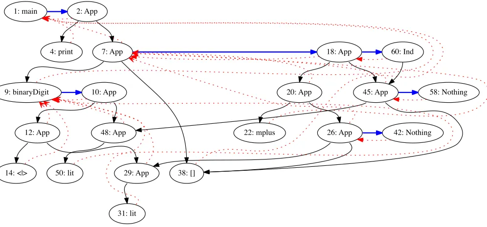
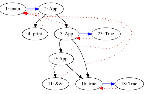
Figure 2 shows the ART for our example. An ART is basically the graph produced by a naive implementation, a simple graph rewriting machine, except that a reduction step does not overwrite a redex by a reduct, but instead connects the redex node with a reduction edge to the reduct node. The nodes of an ART are labelled with function and constructor identifiers or are application nodes Appor indirection nodesInd. For easy referencing we identify every node by a number. There are three sorts of edges:
• Abold reduction edgeleads horizontally from the root of a redex to the root of its reduct. Starting for example at node1, the redexmainreduces to node2, an application ofprint.
1: main 2: App
4: print 7: App
9: binaryDigit
18: App
38: [] 10: App
12: App 48: App
14: <|> 29: App
20: App 45: App 60: Ind
22: mplus 26: App 42: Nothing
31: lit
58: Nothing
[image:3.612.60.558.97.329.2]50: lit
Figure 2: Visual representation of the ART for the program of Figure 1.
• Every node except for the start node1: mainis part of a reduct. Adotted parent edgeleads from every node to the root of its redex. For example, the parent of38: []is 1: main.
The relative order of node identifiers is determined by the lazy evaluation strategy, but the edge structure of an ART is independent of the evaluation strategy. An ART can also represent an eager computation; then every application node always has two outgoing component edges.
An ART contains detailed information for debugging or under-standing how a program works. In general, the ART is far too large and complex to be displayed in its entirety. Hence Hat provides various viewing tools for the ART. Each viewer enables the pro-grammer to interactively explore a computation in a different way, seeing limited information at a time.
Hat transforms a Haskell program into a self-tracing Haskell program. When the latter program is executed, it has the same observable behaviour as the original but in addition generates an ART in a file. To generate all the edges connecting the nodes, Hat’s transformation is rather complex and changes all data types and types of all expressions in a program (Section 2.2).
In this paper we present a much simpler method for obtaining the very same ART for a Haskell program. A new program transforma-tion changes only functransforma-tion bodies and leaves all types in a program unchanged. The transformation applies semantic identity functions, which produce side-effects using the functionunsafePerformIO, to subexpressions. When the value of a subexpression is demanded, then the effect is produced, but otherwise the computation pro-ceeds like in the original program, preserving the lazy evaluation
order. The side-effects record a sequence of events. Through a sin-gle traversal of this sequence from beginning to end we can later reconstruct the ART.
Our method was inspired by the Haskell object observation debugger Hood (Gill 2001). The method is related to our earlier work on algorithmic debugging (Faddegon and Chitil 2015, 2016).
The paper makes the following contributions:
• Type- and semantics-preserving tracing combinators for instrumenting code such that during a computation an informative sequence of events is produced (Section 3). • A simple program transformation that introduces the
trac-ing combinators into a program (Section 4).
• An efficient translation of a sequence of events into an ART (Section 5).
• A prototype implementation for a small subset of Haskell (Section 6).
2
OUTLINE: PROBLEM AND SOLUTION IDEA
The ART was designed as a universal trace for lazy functional programs that contains the information to enable multiple different views of a computation (see Section 9). Sharing within the graph minimises the size of an ART, benefiting both generation time and storage space. Because of the size of an ART — it commonly has millions of nodes — and to decouple trace generation from multiple separate viewing tools, Hat generates the ART in a file.
2.1
The ART Data Structure
type ART = Map NodeId TNode type NodeId = Int
noId = -1
type Name = String type Arity = Int data TNode =
TApp {tred::NodeId,tparent::NodeId, tleft::NodeId,tright::NodeId}
| TVar {tred::NodeId,tparent::NodeId,tname::Name} | TCon {tparent::NodeId,tname::Name,tarity::Arity} | TInd {tparent::NodeId,tind::NodeId}
Figure 3: The ART Data structure.
17→TVar {tred=2, tparent=0, tname="main"} 27→TApp {tred=-1, tparent=1, tleft=4, tright=7} 47→TVar {tred=-1, tparent=1, tname="print"} 77→TApp {tred=18, tparent=1, tleft=9, tright=38} 97→TVar {tred=10, tparent=1, tname="binaryDigit"} 107→TApp {tred=-1, tparent=9, tleft=12, tright=48} 127→TApp {tred=-1, tparent=9, tleft=14, tright=29} 147→TVar {tred=-1, tparent=9, tname="<|>"} 187→TApp {tred=60, tparent=7, tleft=20, tright=45} 207→TApp {tred=-1, tparent=7, tleft=22, tright=26} 227→TVar {tred=-1, tparent=7, tname="mplus"} 267→TApp {tred=42, tparent=7, tleft=29, tright=38} 297→TApp {tred=-1, tparent=9, tleft=31, tright=-1} 317→TVar {tred=-1, tparent=9, tname="lit"} 387→TCon {tparent=1, tname="[]", tarity=0} 427→TCon {tparent=26, tname="Nothing", tarity=0} 457→TApp {tred=58, tparent=7, tleft=48, tright=38} 487→TApp {tred=-1, tparent=9, tleft=50, tright=-1} 507→TVar {tred=-1, tparent=9, tname="lit"} 587→TCon {tparent=45, tname="Nothing", tarity=0} 607→TInd {tparent=18, tind=45}
Figure 4: ART of Figure 2 using types of Figure 3.
An ART is a finite map from node identifiers, we use natural numbers, to trace nodesTNode. There are four different sorts of nodes: application, variable, data constructor and indirection. Every node points to its parent node, that is, the root of the redex whose reduction caused its creation. Both a variable and a constructor node have a name; a constructor also an arity. Both an application and a variable can be the root of a redex and hence they both have a reduction pointer. If there is no reduction, then the reduction pointer isnoId. Finally, both applications and indirections can have components. An application can have two components, left and right. At creation time of an application node these components are still unknown and hence arenoId. In contrast, for an indirection its componenttindis always well-defined. Indirection nodes are needed to ensure that from every reduct its redex can be reached via a parent pointer (Sparud and Runciman 1997a): When an applied function is a projection, an indirection node is added to the ART to represent the result. The parent pointer of the indirection is different from the parent pointer of its component.
Figure 4 shows the ART of our example program using the data types of Figure 3.
2.2
Hat’s Program Transformation
To generate an ART, the Haskell tracer Hat transforms a Haskell program into another Haskell program that, when executed, has the same observable behaviour as the original program but in addition writes an ART describing the computation into a file. File writing is mostly sequential, but because the ART is a graph with cycles, some forward pointers in the ART file have to be updated.
To generate all the graph edges of the ART, the transformation inserts in numerous places in the program a pointer of typeRefExp. Hence the types of all expressions, including function identifiers, change. Every expression of typeTis replaced by an expression of typeR T, where
data R a = R a RefExp
that is, every subexpression is paired with a pointer. Data types change accordingly, for example the definition of the tree type
data Tree a = Empty | Node (Tree a) a (Tree a)
becomes
data Tree a = Empty | Node (R (Tree a)) a (R (Tree a))
Every function type is replaced by the new function type newtype Fun a b = Fun (RefExp -> R a -> R b)
It is substantial work and difficult to implement Hat’s program transformation correctly. Another drawback is that the additional pointers in data structures and function parameters increase the space and time requirements of the program.
2.3
The Idea
During program execution we generate a sequence of events. This sequence could be held in memory or be written sequentially to file. Every new event is added to the end of the current sequence; earlier events are never changed. After the execution has terminated, a single traversal of the sequence from beginning to end translates the event sequence into an ART, which contains both backward and forward pointers.1
In the next sections we assume that a program is just a sequence of top-level function definitions. In Section 7 we discuss further language constructs such as local definitions and constants.
2.3.1 “Identity” Functions with Side-Effects.We can instrument any subexpressionMof a program such that an event is recorded, either just before evaluation ofMor just after evaluation ofM. We just replaceMbyinstPre "begin"M, respectivelyinstPost "end"M, where
instPre :: String -> a -> a
instPre event exp = unsafePerformIO $ do sendEvent event
return exp
instPost :: String -> a -> a
instPost event exp = unsafePerformIO $ do
1We assume that a forward pointer in the ART can be updated in constant time.
exp `seq` sendEvent event return exp
HeresendEvent :: String -> IO aadds the given string as an event to the end of our global sequence of events. The function unsafePerformIO :: IO a -> aturns the event recording into a side-effect, such thatinstPre "begin"andinstPost "end"are polymorphic functions that do not change the type of their argu-ments. For the combinatorinstPostit is important that Haskell provides the parametrically polymorphic functionseq :: a -> b -> bthat forces evaluation to weak-head normal form of its first argument before returning its second argument. Therefore instPrefirst sends the event and then evaluates its argument and postPreevaluates in the opposite order.
2.3.2 Event References Record Expression Nesting. For each func-tion symbol, data constructor and applicafunc-tion we will generate an event. To be able to reconstruct whole nested expressions, events have to be able to refer to each other. Each event in our sequence of events can be identified by a unique event identifier; for simplic-ity we choose as event identifier the position of the event in the sequence, starting with 0. A later event in the sequence can refer to an earlier one by including the event identifier of the earlier one in the later event. Thus we can record an expression having two subexpressions by ensuring that the events for the two subexpres-sions refer to the event of the whole expression. For example, our transformation can replacee1e2byappe1e2, where
app :: (a -> b) -> a -> b app f x = unsafePerformIO $ do
appId <- sendEvent "apply"
return ((instPre ("left" ++ show appId) f) (instPre ("right" ++ show appId) x))
Here it does not matter whether we useinstPreorinstPost. We also note that eventually we should define a new data type for events instead of encoding them as strings.
We ensure that for every subexpression there is an event with a reference to the event of the surrounding expression. Because we add later events at the end of the sequence and never update earlier events, subexpressions have to refer up to events representing larger expressions, but never vice versa. When translating the event sequence in one linear traversal into an ART we have to invert all references to obtain component edges.
2.3.3 Delimit Chains of Reduction.Whenever evaluation of an expression is started, it will be rewritten in a sequence of steps until its value is reached; in terms of ART structure there is a chain of redexes with reduction edges until finally there is a non-redex.2 Our ART of Figure 2 shows five such chains:
1 −−◮ 2
7 −−◮ 18 −−◮ 60 9 −−◮ 10 45 −−◮ 58 26 −−◮ 42
We can instrument any subexpressionMof a program such that an event marking the start is recorded before evaluation of
2We will discuss exceptions, including runtime errors and abortion of a computation
by the programmer in Section 7.4.
myId :: Bool -> Bool myId True = True myId False = False
myNot :: Bool -> Bool myNot True = myId False myNot False = myId True
z :: Bool
z = myNot (myNot True)
Figure 5: A program with expression nesting.
myId :: Bool -> Bool
myId True = instPre "True" True myId False = instPre "False" False
myNot :: Bool -> Bool
myNot True = instPre "apply myId" (myId False) myNot False = instPre "apply myId" (myId True)
z :: Bool
z = ev (instPre "apply myNot" (myNot
[image:5.612.398.472.385.493.2](ev (instPre "apply myNot" (myNot True))) ))
Figure 6: Program with some tracing combinators.
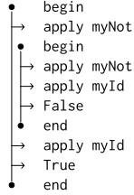
• begin
→ apply myNot • begin
→ apply myNot → apply myId → False
• end
→ apply myId
→ True
• end
Figure 7: Sequence of events generated by evaluation ofz.
the subexpression starts, and another event marking the end is recorded after a value was reached. We just replaceMbyevM, where
ev :: a -> a
ev = instPre "begin" . instPost "end"
App
xs App
rr App
rl <|>
L
L
L
R
R
[image:6.612.104.242.91.189.2]R
Figure 8: Left side of the equation of<|>in Figure 1 as a tree.
constructorTrue. That reduction chain is interrupted by another reduction chain that shows that an application ofmyNotreduced to an application ofmyId, which reduces to the data constructor False.
2.3.4 λ-bound Variables.One additional idea is required to han-dle parameter variables such asxandrlin the example in Figure 1. As Figure 2 demonstrates, an ART contains nodes for variables such aslit,binaryDigitand<|>, but not for parameter variables.3We call the recorded variables let-bound and the unrecorded parameter variablesλ-bound.4For example, the program equation
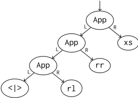
(rl <|> rr) xs = rl xs ’mplus’ rr xs
uses theλ-bound variablesrl,rrandxs. The program execution that yields the ART shown in Figure 2 uses the equation exactly once. Rewriting the equation without infix notation and annotating subexpressions with the corresponding node identifiers of the ART shows more clearly how the equation is used:
((((<|>)14 rl)12 rr)10 xs)7 = ((mplus22 (rl xs)26)20 (rr xs)45)18
The instrumented right-hand sides of the equations formainand
binaryDigityield the ART nodes14,12, etc. that form the left-hand side of the equation for<|>. The instrumented right-hand side of the equation for<|>yields the ART nodes22,26,20, etc. for the right-hand side of the equation. However, additionally that instrumented code has to connect the component edges of theApp
nodes26and45correctly.
We can identify everyλ-bound variable of an equation by a list of left or right branches that indicate their location in a syntax tree of the left-hand side, starting at the root node. The left-hand side of the defining equation of<|>has the syntax tree shown in Figure 8. The tree yields for eachλ-bound variable the following list of branches:
xs: [R]
rr: [L,R]
rl: [L,L,R]
3Originally this decision was made because the ART was inspired by term rewriting. A
term rewriting sequence (computation) contains function identifiers but all parameter variables have been instantiated by substitution. A later justification of this design decision is that function identifiers are essential for understanding a computation, because in contrast to parameter variables they traditionally have meaningful names. As we want to generate an ART, we follow that decision, although recording also parameter variable identifiers would be trivial to implement.
4The naming stems from how a full Haskell program with local definitions inwhere
blocks and class instances would be translated into a coreλ-calculus with a let-binding.
So each event generated for aλ-bound variable contains such a list. The list enables us to add a component edge: the parent of theλ-bound variable is the root node of the left-hand side in the ART and from there we can follow left and right as the branch list specifies to find the root node of the expression bound to the variable. So to add the component edge in the ART, a small part of the already constructed ART needs to be traversed.
2.3.5 Summary.We instrument every subexpression on the right-hand side of an equation. Thus during program execution we record variable and constructor identifiers, but also expression constructs such as applications. These events yield the nodes of the ART.
• The marker eventsbeginandenterdelimit a chain and enable us to construct the reduction edges of the ART. • The nesting of chains reflects the evaluation order, not the
nesting of expressions in the program. So to construct the component edges of the ART, we add an event reference to the surrounding expression to eachEnterevent. The event for aλ-bound variable has a branch list that enables construction of the component edge.
• Finally the parent edges are actually fully determined by the reduction and component edges: the parent of a node in the middle of a chain is the preceding node of the chain (inverse of a reduction pointer); basically the parent of any other node is the same as the parent of the node that they are a component of (inverse of a component pointer).
3
EVENTS AND TRACING COMBINATORS
In the preceding section we discussed our ideas using strings as events and we used simplified tracing combinators. Now we com-bine these ideas to obtain a working tracing system.
Figure 9 gives the definition of events and related types. Every event in an event sequence has a uniqueEventId, which is its position in the sequence.
The subsequence from anEnterevent to its corresponding
Valueevent, without any nested subsequences, describes a chain of reductions. Thus we can later construct reduction edges. AnEnter
event has anEventIdand aBranch, to specify which component of which node it is. This information enables us later to construct component edges.5A constructor event has the name and arity of the constructor, and an event for a let-bound variable has the name of the variable. The event for aλ-bound variable has a list of branches as discussed in the preceding section. Finally, there is the application eventApp.
Figure 10 defines the tracing combinators that we use to generate the event sequence. We assume thatsendEventis a function that takes an event and adds it to the end of the global event sequence; it also returns the uniqueEventIdof that event. The function
runHinitialises the global event sequence, evaluates the given IO-expression, transforms the event sequence into an ART as we will discuss in Section 4 and finally writes the ART to a file with the given name.
5A component edge of an ART always points to the start of a chain. Considering that
type EventId = Int data Branch = L | R type Name = String
data Event =
[image:7.612.351.480.84.687.2]Enter EventId Branch | Value
| Con Name Arity | Var Name | LamVar [Branch] | App
Figure 9: Events recorded in a sequence.
sendEvent :: Event -> IO EventId
runH :: FilePath -> IO a -> IO ()
eval :: EventId -> Branch -> a -> a
eval parent branch x = unsafePerformIO $ do sendEvent (Enter parent branch)
x `seq` sendEvent Value return x
con :: Name -> Arity -> a -> a
con name arity x = unsafePerformIO $ do sendEvent (Con name arity)
return x
var :: Name -> a -> a
var name var = unsafePerformIO $ do sendEvent (Var name)
return var
lamVar :: [Branch] -> a -> a
lamVar pos var = unsafePerformIO $ do var `seq` sendEvent (LamVar pos) return var
app :: (a -> b) -> a -> b app f x = unsafePerformIO $ do
eventId <- sendEvent App
return ((eval eventId L f) (eval eventId R x))
Figure 10: Tracing combinators.
The combinatorevalmarks the beginning and end of a chain of reductions as discussed in Section 2.3.3; it just takes anEventIdand Branchas parameters, to include them in theEnterevent. Com-binatorsconandvargenerate constructor and let-bound variable events. The combinatorlamVargenerates the event for aλ-bound variable. The definition first forces the evaluation of the variable via seq, so that the chain of computation for the variable is recorded in the event sequence before theLamVarevent is added. Finally the
• 0: Enter 0 L
→ 1: Var "main"
→ 2: App
• 3: Enter 2 L
→ 4: Var "print"
• 5: Value
• 6: Enter 2 R
→ 7: App
• 8: Enter 7 L
→ 9: Var "binaryDigit"
→ 10: App
• 11: Enter 10 L
→ 12: App
• 13: Enter 12 L → 14: Var "<|>" • 15: Value • 16: Value • 17: Value
→ 18: App
• 19: Enter 18 L
→ 20: App
• 21: Enter 20 L → 22: Var "mplus" • 23: Value • 24: Value • 25: Enter 20 R
→ 26: App
• 27: Enter 26 L • 28: Enter 12 R
→ 29: App • 30: Enter 29 L
→31: Var "lit" • 32: Value • 33: Value
→ 34: LamVar [L,L,R] • 35: Value
• 36: Enter 26 R • 37: Enter 7 R
→ 38: Con "[]" 0 • 39: Value → 40: LamVar [R] • 41: Value
→ 42: Con "Nothing" 0 • 43: Value
• 44: Enter 18 R
→ 45: App
• 46: Enter 45 L • 47: Enter 10 R
→ 48: App • 49: Enter 48 L
→50: Var "lit" • 51: Value • 52: Value → 53: LamVar [L,R] • 54: Value • 55: Enter 45 R
→ 56: LamVar [R] • 57: Value
→ 58: Con "Nothing" 0 • 59: Value
→ 60: LamVar [R]
• 61: Value
• 62: Value
combinatorapprecords an application event. It wraps the combina-torevalaround both components of the application. This collabo-ration of the two combinators ensures that the component structure of expressions is recorded in the trace. The combinatorevalis used only in the definition ofappand for starting the computation of a complete program in the definition ofrunH. The combinatorapp is the only combinator that uses the unique identifier returned by sendEvent.
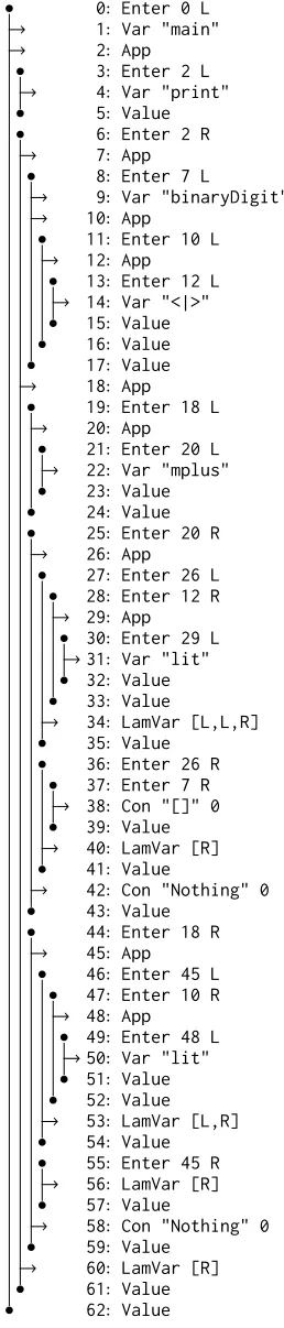
Figure 11 shows the complete event sequence for our program from the Introduction. The markings on the left emphasise the chains of reductions just as in Figure 7. The whole sequence is bracketed by anEnter 0 Land aValueevent that were generated byrunH. The additional information of anEnterevent determines for a chain to which component of which application it belongs. EveryAppevent is followed directly by anEnterevent for its left component, the applied function. AnEnterevent for its right component, the argument of the function, may appear later in the event sequence, but will only appear if it is demanded.
4
PROGRAM TRANSFORMATION
A transformation that inserts the tracing combinators instruments a program for tracing. Figure 12 shows the result of transforming our introductory program of Figure 1. A module import for the tracing libraryHatLightthat defines the tracing combinators is added. The standard libraryPreludeis hidden and instead a trac-ing version of it,HatPrelude, is imported. All type definitions and type signatures remain unchanged, just like the left-hand sides of equations that define functions. However, all expressions are trans-formed by inserting tracing combinators. That transformation is straightforward, except that for each use of aλ-bound variable a list of branches is needed, which is obtained from the left-hand side of the equation as described in the previous section. The combinators apphniare variants ofappthat apply a function tonarguments. The functionmainusesrunHand starts by recording its own vari-able identifier in the event sequence. Executing this program yields the event sequence shown in Figure 11.
5
TRANSLATION FROM EVENT SEQUENCE
TO ART
When we generate an event sequence, we never update any event; we only join new events at the end. Thus an event sequence has backwards references, namely theEventIdof eachEnterevent, but no forward references. We translate such an event sequence into an ART which also has forward references, namely the component and reduction pointers. Translation traverses the event sequence once from beginning to end. From each event a new ART node is created, except forEnterandValueevents. For simplicity we use theEventIdof an event as theNodeIdof the corresponding ART node. Hence there are no ART nodes with theEventIds ofEnter orValueevents. The generation of the ART is mostly a sequential writing processes: If the ART is stored in a sequential data structure such as a file, then new nodes can be joined at the end; however, a few updates and also reading operations of the existing partial ART are needed.
Figure 13 defines the translation as a Haskell functionmkArt. During the traversal the translation functiongokeeps track of a
import HatLight
import qualified Prelude import HatPrelude
type Recogniser = [Char] -> Maybe [Char]
lit :: Char -> Recogniser
lit x [] = con "Nothing" 0 Nothing lit x (y:ys) =
app3 (var "if" ifThenElse) (app2 (var "==" (==))
(lamVar [L,R] x) (lamVar [R,L,R] y)) (app (con "Just" 1 Just) (lamVar [R,R] ys)) (con "Nothing" 0 Nothing)
(<|>) :: Recogniser -> Recogniser -> Recogniser (<|>) rl rr xs =
app2 (var "mplus" mplus)
(app (lamVar [L,L,R] rl) (lamVar [R] xs)) (app (lamVar [L,R] rr) (lamVar [R] xs))
mplus :: Maybe a -> Maybe a -> Maybe a mplus Nothing mr = lamVar [R] mr mplus ml _ = lamVar [L,R] ml
binaryDigit :: Recogniser binaryDigit =
app2 (var "<|>" (<|>))
(app (var "lit" lit) (con "'0'" 0 '0')) (app (var "lit" lit) (con "'1'" 0 '1'))
main =
runH "Recogniser" Prelude.$ var "main" Prelude.$ app (var "print" print)
(app (var "binaryDigit" binaryDigit) (con "[]" 0 []))
Figure 12: Transformed Example Program.
stack ofChains and theNodeId=EventIdof the event currently
being processed. The functionwriteConnectadds one node to the ART data structure and modifies it in other places; that is, if the newly written node is the beginning of a chain, then the node that it is an argument of is updated (writeArg); otherwise it is a later entry in a chain and the reduction pointer of the preceding node is updated (updateReduction). Hence a component pointer always points to the first node of a reduction chain.
data Chain = Context NodeId Branch | Last NodeId
mkArt :: [Event] -> ART
mkArt es = go es [] 0 Map.empty
go :: [Event] -> [Chain] -> NodeId -> ART -> ART go (Enter a b : es) cs id art =
go es (Context a b : cs) (id+1) art go (Value : es) (c:cs) id art =
go es cs (id+1) art
go (Con name arity : es) cs id art = writeAndGo es cs id
(\p -> TCon p name arity) art go (App : es) cs id art =
writeAndGo es cs id
(\p -> TApp noId p noId noId) art go (Var name : es) cs id art =
writeAndGo es cs id
(\p -> TVar noId p name) art
go (LamVar d : es) (Context a b : cs) id art = go es (Last n : cs) (id+1) (writeArg a b n art) where
n = directionLookup (getParent a art) d art go (LamVar d : es) cs id art =
writeAndGo es cs id
(\p -> TInd p (directionLookup p d art)) art go [] [] _ art = art
writeAndGo :: [Event] -> [Chain] -> NodeId -> (NodeId -> TNode) -> ART -> ART writeAndGo es (c:cs) id newNode =
go es (Last id : cs) (id+1) . writeConnect c id newNode
writeConnect :: Chain -> NodeId ->
(NodeId -> TNode) -> ART -> ART writeConnect (Context a b) id newNode art =
writeArg a b id .
Map.insert id (newNode (getParent a art)) $ art writeConnect (Last l) id newNode art =
updateReduction l id .
Map.insert id (newNode l) $ art
Figure 13: Translation of an event sequence into an ART.
Contexton the stack, translation of aValueevent removes a chain from the stack.
The translation ofCon,Varand evenAppevents is relatively simple. Each gives rise to the construction of a corresponding ART node.
The translation of aLamVarevent is more complex. Translation uses the functiondirectionLookup, which given the node that rep-resents the root of the left-hand side for thisλ-bound variable plus the list of branches and the current partial ART, returns the node that is the root of the value of the variable. We have to distinguish two cases:
• If we are at the beginning of a chain, then theλ-variable is a component, not the right-hand side of an equation. We get the parent node of the context node; that is the root of the left-hand side of the equation in the ART. From that nodedirectionLookupobtains the beginning of the chain of theλ-bound variable. The argument specified by theContextis updated with the node beginning that chain. That node is used for updating the argument specified by theContext.
For example, theλ-bound variablexsof the equation for<|>in Figure 1 has the branch list[R]. Hence the right argument of node26is the node38in Figures 2 and 4. • If we are in the middle of a chain, then theλ-variable is
the right-hand side of an equation. That equation defines a projection. From that last nodedirectionLookupobtains the beginning of the chain of theλ-bound variable. That node is the component of the new indirection node that is added to the ART, connected by reduction pointer from the last node.
For example, the right-hand side of the first equation ofmplusin Figure 1 is just theλ-bound variablemr, which has the branch list[R]. Therefore the reduction pointer of node18points to an indirection node60whose component is node45in Figures 2 and 4.
6
A PROTOTYPE: HATLIGHT
HatLight is our prototype implementation of the new method for creating an ART. HatLight is mainly a Haskell library that defines the tracing combinators and the translation from event sequences to an ART. Both event sequence and ART are data structures in memory, not in files. HatLight outputs the event sequence and ART, but also writes the ART into a file using the DOT graph description language.6Thus the ART can be visualised with a tool such as GraphViz.7HatLight also includes a tracing standard library, which includes some frequently used functions and types. Currently HatLight consists of approximately 570 lines of Haskell code.
All the transformed programs, event sequences, ART data and visualisations of the ART in this paper have been obtained with HatLight. The definitions of the combinators and the translation are excerpts of HatLight.
To gain an insight into the overhead of tracing, we modified our prototype to write the event sequence into a file. The event sequence contains all information needed to construct an ART and it is of similar size. We measured the runtime of the original and traced versions of two programs, each with two different parameters. The programnfibdetermines by simple, exponential recursion the Fibonacci number of the parameter. The programpermsoutputs all permutations of the list of numbers from 1 to the parameter. It uses the definitions given in Section 9.4 of Hutton (2016); all list functions, includingmap,(++)andconcatare traced. The table in Figure 14 gives the measurements obtained on a MacBook Air with flash storage, after compilation with the Glasgow Haskell compiler8 version 7.8.3 with flag-O2.
6https://en.wikipedia.org/wiki/DOT_(graph_description_language) 7https://www.graphviz.org
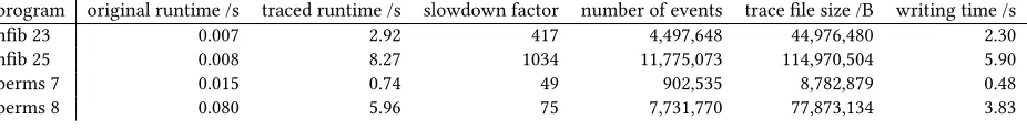
program original runtime /s traced runtime /s slowdown factor number of events trace file size /B writing time /s
nfib 23 0.007 2.92 417 4,497,648 44,976,480 2.30
nfib 25 0.008 8.27 1034 11,775,073 114,970,504 5.90
perms 7 0.015 0.74 49 902,535 8,782,879 0.48
[image:10.612.78.541.86.145.2]perms 8 0.080 5.96 75 7,731,770 77,873,134 3.83
Figure 14: Tracing measurements for two example programs.
The slowdown factor of runtime is substantial. The table also shows that the computations produce huge trace files, each of which contains many events. Therefore we wrote a Haskell program that just writes the same number of lines; each line is a constant string of length 9, so that the file size is similar to the corresponding event sequence file. The last column in the table gives the runtimes of this program. Thus we see that more than half of the runtime of a traced program is needed just for writing the event sequence file. So to reduce the slowdown factor in the future, we will have to speed up file writing. Our prototype uses the simple but inefficient line
hPutStrLn handle (show event)
to write an event into the file.
Nonetheless, the runtime overhead and the file sizes clearly demonstrate that we should not trace every reduction of a program. In Section 8 we will discuss how we can trace only part of a program.
7
COVERING THE COMPLETE LANGUAGE
Since 2002 Hat works for all of Haskell 98 plus a few common exten-sions such as multi-parameter classes and functional dependencies. Hence its definition of the ART covers all of Haskell. However, we still have to ensure that our new method for generating an ART works for all of Haskell.
7.1
Types and Classes
Haskell has a complex system of types and classes. Because our transformation changes expressions without changing their types, we do not transform type or class definitions, only the definitions of bodies of methods in class instances. Hence our method is agnostic of the type and class system and its implementation is not affected by any extensions of that system.
7.2
Local Definitions
Consider the following function definition that makes use of a locally defined function. The functionsnocappends an element to the end of a list.
snoc :: a -> [a] -> [a] snoc x xs = go xs
where go [] = [x]
go (y:ys) = y : go ys
We can transform the right-hand side of each defining equation as before, but we face one problem: The variablexis used in the body of the definition of the local functiongo, but it isλ-bound on the left-hand side of the enclosing definition of the top-level functionsnoc. Hat generates an ART for this program, but it was
noticed that presenting applications of a local function without the values of its free variables can yield to confusing views. For example,hat-observecould produce an output such as
go [] = [0] go [] = [42]
However, Hat’s ART contains more information than the ART data structure given in Figure 3. Every variable node has a Boolean flag that indicates whether this is a local variable that may have free variables. Every variable node stores the beginning and end of its definition in the source code. Thus it is easy to determine whether one variable is defined locally within the definition of another variable. Although the chain of parents (parent, grandparent, grand-grandparent, etc.) of a node is information about the dynamics of a computation, for a local variable the chain of parents includes the redex roots of all enclosing variables. Thus the ART has the information to determine for any local variable the redex roots of all its enclosing variables. Hencehat-observecan produce an output like
(snoc 0 []).go [] = [0] (snoc 42 []).go [] = [42]
We can extend HatLight to also record for every let-bound vari-able a Boolean flag and information about the beginning and end of its definition in the source. Furthermore, HatLight needs to include in the event for aλ-bound variable a counter of how many levels of enclosing redexes to go up before following the list of branches as described in Section 2.3.4;9Thus HatLight could generate the correct ART also for programs with local definitions as above.
7.3
Constants
Although by definition Haskell is only a non-strict language, all implementations provide a lazy semantics and thus ensure that every constant is computed at most once with its value being shared by all use occurrences. We call a let-bound variable in a program a constant, if it appears alone on the left-hand side of its defining equation, that is, it is not a function identifier with parameters on the left-hand side.10In our introductory examplebinaryDigitand mainare constants and they are the only constants. Because each of these constants is used only once, our tracing method works fine. However, if a constant is used twice or more, then the tracing method fails. Consider
true :: Bool true = True
9This counter corresponds to the de Bruijn index ofλ-calculus.
10There is a difference between the termconstantand the established termconstant
1: main 2: App
4: print 7: App
9: App 19: true
21: True
[image:11.612.52.298.95.249.2]11: && 15: true 16: True
Figure 15: An ART that is incomplete because of a constant.
1: main 2: App
4: print 7: App
9: App
16: true 25: True
11: && 18: True
Figure 16: An ART that shares the constanttruecorrectly.
main = print (true && true)
With our method we obtain the incomplete ART shown in Figure 15 The node15: truereduces to the result16: True, but there is no reduction edge for node19: true. The reason for the problem is simple: the constantboolis only evaluated once and the resulting valueTrueis stored and not recomputed when the value oftrue is demanded again; however, our tracing works by side-effects that only happen when computation happens. This effect may not only lead to missing information in an ART, but we may obtain an invalid event sequence that cannot be translated into an ART at all. That happens for example for the following program:
pair :: (Int,Int) pair = (6,7)
fst (x,_) = x snd (_,x) = x
main = print (fst pair * snd pair)
The first occurrence ofpairyields a reduction chain in the event sequence, but the second occurrence does not. However, the body of the functionsndis aλ-bound variable with branch list[R,R]. Fol-lowing this direction in the partially constructed ART fails, because there is no second pair constructor in the ART.
Hat handles constants (Chitil et al. 2003). The computation of a constant is shared in its ART. The ART has a special node for the use occurrence of a constant. That node is similar to an indirection; its component pointer points at the single shared value of the constant. There is no single parent for a constant, because the constant can be used by many redexes of the computation. In early versions of Hat the parent pointer of a constant does not point to any of its parents; in later versions of Hat a constant has a list of parent pointers, one for each parent redex. It is unclear whether the additional time and space overhead for storing this list is worthwhile for the views.
We recently enhanced our new method for generating an ART to handle constants. Because a constant is computed only once, its computation is recorded only once in the event sequence and thus the ART. We added a new event and new combinator for each use of a constant. Thus we can connect several uses of a constant to the single chain for the constant. Figure 16 shows the resulting ART for the first example of this section. In our current version a constant has no parents. This enhancement also works for recursively defined constants, but it is still experimental, because it may not work well in combination with untraced code, which we discuss in Section 8.
7.4
Exceptions
A computation of a program may explicitly raise an exception. Any runtime error and also the abortion of a computation by the programmer raises an exception. We can handle these by adding an exception handler in the combinatoreval. When an exception is raised all reduction chains that are still open can be terminated with an exception value and the eventValue.
7.5
Desugaring
Haskell has many language features that can be desugared into a small subset of the language. For example, a list comprehension can be desugared into the use of a few list combinators. However, for the end user it is desirable that a view of the ART shows an expression as it is in the program. That will require extending the ART data structure and extending every view accordingly.
Desugaring is a temporary solution to obtain a tracing system for Haskell quickly, but in the long term every language construct will need to be supported directly.
7.6
Challenges
[image:11.612.53.293.303.459.2]By definition Haskell is a sequential language, but its most popu-lar compiler, the Glasgow Haskell compiler, provides it with several different application interfaces for concurrent programming. Our lightweight tracing method generates a sequence of events; the order of these events is essential for reconstructing the ART. Hence our method works only for tracing a sequential computation, at best a single thread of a concurrent computation. The most simple extension to handle many concurrent threads would assume to have at runtime access to an identifier of the current thread and add this identifier to every event. Thus for every thread an event se-quence could be determined and an ART-like trace be reconstructed. In practice, much further research will be needed to find a good way of presenting a concurrent computation to the user, probably specific to the particular concurrency application interface that the program uses.
8
UNTRACED CODE
Our new method works well for transforming and then tracing the computation of a complete program. However, in general pro-grammers do not want to trace the computation of all code of a program. When a program uses a library, the programmer usually does not want to see the details of library-function computations. Additionally, tracing creates a time and space overhead that the programmer wants to limit to the parts of the program that they are interested in.
Hat also transforms untraced code, using a slightly different transformation and different combinators. That way untraced code has the same transformed types as traced code and both can eas-ily be combined. Hat’s method is pragmatic but not perfect: the untraced code still writes some superfluous information into the ART file while missing out some essential parts. Because our new method for generating an ART leaves the types of all expressions unchanged, combining transformed and untransformed code is not hindered by changes in types.
It is highly desirable to combine transformed and untransformed code. Untransformed code will always be more efficient and it may use some language features that the program transformation does not (yet) support. Also, transformed code still has to use some untransformed primitive functions, for example for arithmetic and input/output.
Combining traced and untraced code requires some thought. The computation of a function in untraced code is not traced, but that function returns a value to the traced world. Hence that value needs to be recorded in the trace. Both the Hat and the HatLight program transformations can easily handle a call to an untraced first-order function by wrapping it in a combinator that records the result value in the trace when it is returned from the function.
In a higher-order programming language, that value may be a function or a data structure that contains functions. The ART represents a functional value as a function identifier or a partial application of a function identifier. It is unclear how any wrapper could record that function identifier in the ART. Worse, if that function identifier is defined in untraced code, in particular if it is a local function of some black-box library, it should not appear inside the ART. So the definition of the ART does not fit with the concept of black-box untraced code.
We see the solution to the problem in representing a functional value that is returned from untraced code not intensionally, but extensionally, that is, as a finite map from arguments to results. For example for the program
main = print (map (+ 1) [1,2,3])
the value of(+ 1), and thus also the argument for the function map, can be represented as
{1 7→ 2, 2 7→ 3, 3 7→ 4}
The algorithmic debuggerhoed-pureuses this representation of functional values and it is also based on first generating a sequence of events which afterwards is translated into its computation tree (see Section 9.3). Hence merging the method ofhoed-pureinto HatLight is a feasible future goal.
9
RELATED WORK
9.1
ART and Hat
The Haskell tracer Hat11produces an ART for a Haskell program. The design of the structure of an ART started with the redex trail trace developed by Sparud and Runciman (1997a,b). That redex trail only allowed trace exploration as later implemented inhat-trail and described in Section 9.1. A comparison of three different trac-ing systems for Haskell lead to the conclusion that different views of a computation are useful (Chitil et al. 2001). A small addition to the redex trail structure, namely reduction pointers, yields an augmented redex trail (ART) that can support all three views. Wal-lace et al. (2001) implemented this addition and the three views . Claessen et al. (2003) give the most extended examples of what Hat does from the user’s point of view. Later Chitil (2005) and Silva and Chitil (2006) explored further views and uses of the ART. Chitil et al. (2003) define Hat’s program transformation for generating an ART and later Chitil and Luo (2007) defined the ART structure formally and proved basic properties.
Multiple Views.To appreciate the structure of the ART, we briefly review some of the views of an ART that Hat provides.
The viewing toolhat-observeis inspired by Hood (see Sec-tion 9.3). For a given funcSec-tion identifier it lists all the arguments that the function was applied to during a computation plus its results. For example, for the function identifierlitit shows
lit _ [] = Nothing
removing duplicates, and for the function identifiermplusit shows mplus Nothing Nothing = Nothing
An observation can be obtained from a single linear traversal of the ART. Whenhat-observeis started, it first creates an index of every identifier occurring in the ART to speed up every later search. Component edges enable reconstruction of expressions and reduction edges point to the result value of a redex.
The viewing toolhat-trailallows exploring the history of an expression backwards: it tells that the argumentNothingof printwas created by the reduction ofmplus Nothing Nothing. The secondNothingof that redex was created by the reduction of lit _ []. The first application of that redex was created by the reduction ofbinaryDigit. FinallybinaryDigitwas created by the reduction ofmain. In every step the programmer can select any
1: main = print Nothing
7: (lit _ <|> lit _) [] = Nothing
9: binaryDigit = lit _ <|> lit _
26: lit _ [] = Nothing 45: lit _ [] = Nothing
[image:13.612.61.554.83.166.2]18: mplus Nothing Nothing = Nothing
Figure 17: Evaluation dependence tree (EDT) obtained from the ART shown in Figure 2.
subexpression of a given expression and ask for its parent. Below a selected subexpression is underlined and its parent is given in the subsequent line:
print Nothing
<- mplus Nothing Nothing <- lit _ []
<- binaryDigit <- main
Thushat-trailenables exploring a computation backwards; de-bugging goes from a noticed failure backwards to the program defect that caused it. Parent edges are essential forhat-trail’s functionality;hat-trailreconstructs expressions from component edges.
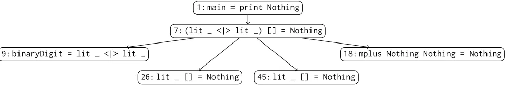
The viewing toolhat-detectis an algorithmic debugger for semi-automatically locating a defect in a program. At the heart of algorithmic debugging is a computation tree, a structured repre-sentation of a computation. Figure 17 shows the computation tree, an evaluation dependence tree, constructed byhat-detectfor our example. Every node is a computation statement: a redex plus its result value (we considerprint Nothingas a value of typeIO ()). Here we include the ART node identifier of the redex in each tree node to emphasise the relationship. The tree gives insight into the computation, but because our program shows no failure, we cannot do any debugging. The toolhat-detectconstructs the evaluation dependence tree on the fly from the ART, using all three sorts of edges.
Most debuggers used in practice, especially for imperative pro-grams, are stepping debuggers. A stepping debugger is a very spe-cial instance of an algorithmic debugger; the stepping debugger only allows a linear, forward traversal of the computation tree. This relation between stepping debugger and computation tree is central to the work of Braßel et al. (2007), which we discuss later. The ART could be used as basis for a stepping debugger similar to the one of Braßel et al. (2007).
Many other uses of an ART have been discussed and/or imple-mented, for example, a virtual stack trace and dynamic program slicing.
A Structural Differences.The ART structure as shown in Figure 2 and generated by our new method differs from Hat’s ART in one point: A component pointer isnoId, when the component was never demanded during the computation. In contrast, Hat’s ART always has a valid component pointer to the root of an (unevaluated) expression. Recording such an unevaluated expression would be possible in principle, but substantially complicate our method. The
additional information about unevaluated expressions seems of little use. To prevent information overload, displayed expressions should avoid any unnecessary information, and Hat’s viewing tools already offer showing such unevaluated expressions just as _.
9.2
Other Algorithmic Debuggers for Lazy
Functional Languages
Besideshat-detect, several algorithmic debuggers (Shapiro 1983) for Haskell have been developed. Nilsson and Sparud (1997) define the evaluation dependence tree (EDT) as a suitable computation tree for algorithmic debugging of lazy functional programs. Nilsson’s algorithmic debugger Freja generates an EDT (Nilsson 1998, 2001). Freja does not generate a more general trace like the ART. Freja is a complete compiler for a subset of Haskell and compiler and runtime system together enable the generation of the EDT. Therefore debug-ging with Freja has only modest runtime overheads, but a complex tracing architecture integrated with a compiler makes supporting a large and evolving programming language such as Haskell very hard. In contrast our lightweight method permits us better to ex-plore the design space of tracing and will hopefully enable us to build the first omniscient debugger that will be used for real-world Haskell programs. Freja already handles many language features discussed in Section 7. In particular, Freja records the names of all variables, includingλ-bound variables, and for each locally de-fined variable it records the set of its free variables together with their values. Thus Freja can provide inspiration for an alternative, possibly more friendly user interface to some language features. Freja requires all higher-order functions to be traced, even though the workings of trusted higher-order functions is not recorded; in contrast we outlined in Section 8 how we plan to use untraced higher-order functions.
Pope (2005, 2006) built the algorithmic debugger Buddha for Haskell. Generation of the computation tree is based on program transformation, which, however, is still integrated with an existing compiler, the Glasgow Haskell compiler. Buddha can represent functional values as finite maps and Pope stated that a computation tree with functional values as finite maps has to have a structure that is different from the EDT. Subsequently Chitil and Davie (2008) defined the new computation tree structure formally by relating it to the ART, named it the function dependence tree (FDT), and proved its soundness for algorithmic debugging.
9.3
Hood and Hoed
programs, which he implemented in his Haskell debugging library Hood (Gill 2001). A programmer using Hood annotates their pro-gram with theobservecombinator. At runtime these annotations generate a sequence of events. Finally, when computation termi-nates, the Hood library reconstructs observed values from the se-quence of events. These values can be values of data types, that is, applications of data constructors and primitive values such as 42and’a’, or functional values. A functional value is represented extensionally, that is, as a finite map from arguments to results, as we discussed in Section 8. To sum up, Hood does not generate any trace structure from its sequence of events, but a set of values.
We identified and generalised Hood’s use of “identity” functions with side-effects and its use of event references to record expres-sion nesting. Hood’sEnterevents inspired our novel method of delimiting chains of reductions in the event sequence. Hood does not record such chains; it does not need them for observing only values.
Faddegon and Chitil (2015) combined Hood’s instrumentation with the cost centre stacks of the profiling system of the Glasgow Haskell compiler to obtain a computation tree for algorithmic de-bugging of Haskell programs. The implementationhoed-stack
uses Hood’s event sequence to obtain computation statements as nodes of the computation tree and the cost centre stacks are used to connect these nodes to a tree. The computation tree is a function dependence tree, not an evaluation dependence tree (cf. Section 9.2). Subsequently Faddegon and Chitil (2016) discovered that cost centre stacks are not needed, but that the very same sequence of events that Hood generates already contains sufficient information to connect the nodes of computation statements to a tree. The central insight is that events come in pairs, anEnterevent is later followed by an event describing the weak-head normal form of a value. From the nesting structure of these event pairs the structure of the computation tree can be obtained. Because of higher-order functions, the relationship between nesting of event pairs and the computation tree structure is quite complex. The implementation of this algorithmic debugger is calledhoed-pure.
Here, in this paper, we follow Hood in instrumenting a program with combinators that generate a sequence of events. However, Hood traces only values and except for function identifiers so does Hoed. To obtain the richer information needed for an ART, we use a richer set of events. For example, we have events for both let-andλ-bound variables. Instead of the event pairs of Hood we have chains of events, starting with anEnterand ending with aValue
event, but with an unbound number of events in between. Hood’s and Hoed’s program annotations are far more lightweight than the instrumentation introduced by our program transformation. Hoed requires only one annotation in the definition of each function of interest. It’sobservecombinator recursively traverses a data struc-ture while recording it in the sequence of events. In contrast, we annotate every subexpression with a combinator. Thus we record a value when it is constructed by the program (the data constructor is instrumented), whereas Hood and Hoed record a value when that value passes through theobservecombinator which otherwise behaves like the identity function.
Hood and Hoed have the great advantage that they require an-notating only functions of interest; most of a program may be left
unchanged. The connection of computation tree nodes based on nested event pairs works even when an arbitrary number of un-traced function calls are performed in between. In contrast, our method for constructing an ART is based on transforming the com-plete program. This whole-program tracing is the premise for being able to transform the event sequence into the ART, a single con-nected graph. As we discussed in Section 8, extending our method to work with untransformed modules will probably require combining it with the method ofhoed-pure.
Finally our method for constructing an ART has the advantage that it preserves sharing of expressions in the heap of the instru-mented program, whereas theobservecombinator loses sharing. Hence for Hood and Hoed the execution of an annotated program can require more space and the event sequence contains much duplication, compared to the ART.
9.4
Other Debuggers for Lazy Functional
Languages
Perera et al. (2012) define another tracing model for lazy functional programs that is based on program slicing. They prove several desirable properties for their approach. It would be interesting to establish whether the ART meets similar properties, which the work of Silva and Chitil (2006) suggests.
Marlow et al. (2007) describe a different approach to debugging Haskell programs. They describe how a traditional stepping debug-ger can work and be implemented for a lazy functional language.
Braßel et al. (2007) present a debugging approach for Haskell that views a computation in a combination of a traditionally stepping debugger and an algorithmic debugger. For eager evaluation these two views are closely related. The central idea is that a small trace states which reduction steps an eager evaluator should skip to perform exactly the same computations as a lazy evaluator. This trace is generated by an initial lazy computation of the program. The viewing tool then uses an eager evaluator of Haskell together with the small trace to provide a view of eager evaluation that “magically” skips unnecessary steps. This approach fits well with our observation that the ART structure is independent of the order of evaluation. The main obstacle in practice is that for a lazy language there is hardly ever an eager evaluator available but it must be implemented from scratch.
10
CONCLUSIONS
We have presented a new method for generating a detailed trace of a lazy functional computation. We have shown that the simple idea of instrumenting a high-level program such that it generates events at well-defined points of the computation can yield detailed information about how a computation works; this technique, first introduced by Gill (2001), clearly has many potential application areas. We have described and justified every step of the new method. Our implementation HatLight establishes that the method works.
We could complete HatLight to write the ART into a file in the same format as used by Hat, such that all of Hat’s viewing tools could be used. However, our aim in the near future is to use HatLight as an experimental platform for modifications and extensions as discussed in Sections 7 and 8. For that purpose HatLight needs to stay small and allow for useful variations of the ART that are incompatible with Hat. The difference discussed in Section 9.1 is already such a variation.
With different combinators our method should also work for strict functional programming languages. However, because these languages are generally not pure, recording of side-effects in the ART will be important. Hat currently supports basic input-output effects in its tracing and ART, but further work in this area will be required.
ACKNOWLEDGMENTS
We thank the reviewers, in particular Henrik Nilsson, for their valuable comments and helpful suggestions.
REFERENCES
Bernd Braßel, Michael Hanus, Sebastian Fischer, Frank Huch, and Germán Vidal. 2007. Lazy call-by-value evaluation. InICFP ’07: Proceedings of the 2007 ACM SIGPLAN International Conference on Functional Programming. 265–276.
Olaf Chitil. 2005. Source-based trace exploration. InImplementation and Application of Functional Languages, 16th International Workshop, IFL 2004 (LNCS 3474), Clemens Grelck, Frank Huch, Greg J. Michaelson, and Phil Trinder (Eds.). Springer, 126–141. Olaf Chitil and Thomas Davie. 2008. Comprehending Finite Maps for Algorithmic Debugging of Higher-Order Functional Programs. In10th International ACM SIG-PLAN Symposium on Principles and Practice of Declarative Programming, PPDP 2008. ACM, 205–216.
Olaf Chitil and Yong Luo. 2007. Structure and Properties of Traces for Functional Programs. InProceedings of the 3rd International Workshop on Term Graph Rewriting, Termgraph 2006 (ENTCS 176(1)), Ian Mackie (Ed.). 39–63.
Olaf Chitil, Colin Runciman, and Malcolm Wallace. 2001. Freja, Hat and Hood — A Com-parative Evaluation of Three Systems for Tracing and Debugging Lazy Functional Programs. InProceedings of the 12th International Workshop on Implementation of Functional Languages (IFL 2000) (LNCS 2011), Markus Mohnen and Pieter Koopman (Eds.). Springer, Aachen, Germany, 176–193.
Olaf Chitil, Colin Runciman, and Malcolm Wallace. 2003. Transforming Haskell for Tracing. InProceedings of the 14th International Workshop on Implementation of Functional Languages (IFL 2002) (LNCS 2670). 165–181.
Koen Claessen, Colin Runciman, Olaf Chitil, John Hughes, and Malcolm Wallace. 2003. Testing and Tracing Lazy Functional Programs using QuickCheck and Hat. In4th
Summer School in Advanced Functional Programming (LNCS 2638). 59–99. Maarten Faddegon and Olaf Chitil. 2015. Algorithmic Debugging of Real-world Haskell
Programs: Deriving Dependencies from the Cost Centre Stack. InProceedings of the 36th ACM SIGPLAN Conference on Programming Language Design and Imple-mentation. ACM, 33–42.
Maarten Faddegon and Olaf Chitil. 2016. Lightweight Computation Tree Tracing for Lazy Functional Languages. InProceedings of the 37th ACM SIGPLAN Conference on Programming Language Design and Implementation.
Andy Gill. 2001. Debugging Haskell by Observing Intermediate Data Structures.
Electronic Notes in Theoretical Computer Science41, 1 (2001). 2000 ACM SIGPLAN Haskell Workshop.
Graham Hutton. 2016.Programming in Haskell. Cambridge University Press. Simon Marlow, José Iborra, Bernard Pope, and Andy Gill. 2007. A lightweight
interac-tive debugger for Haskell. InHaskell ’07: Proceedings of the ACM SIGPLAN workshop on Haskell. ACM, New York, NY, USA, 13–24.
Henrik Nilsson. 1998.Declarative Debugging for Lazy Functional Languages. Ph.D. Dissertation. Linköping, Sweden.
Henrik Nilsson. 2001. How to Look Busy While Being As Lazy As Ever: The Imple-mentation of a Lazy Functional Debugger.J. Funct. Program.11, 6 (Nov. 2001), 629–671.
Henrik Nilsson and Jan Sparud. 1997. The Evaluation Dependence Tree as a Basis for Lazy Functional Debugging.Automated Software Engineering: An International Journal4, 2 (April 1997), 121–150.
Roly Perera, Umut A. Acar, James Cheney, and Paul Blain Levy. 2012. Functional Programs That Explain Their Work. InProceedings of the 17th ACM SIGPLAN International Conference on Functional Programming (ICFP ’12). ACM, New York, NY, USA, 365–376.
Bernie Pope. 2005. Declarative Debugging with Buddha. InAdvanced Functional Programming, 5th International School, AFP 2004 (LNCS 3622). Springer Verlag, 273–308.
Bernie Pope. 2006.A Declarative Debugger for Haskell. Ph.D. Dissertation. The Univer-sity of Melbourne, Australia.
E. Y. Shapiro. 1983.Algorithmic Program Debugging. MIT Press.
Josep Silva and Olaf Chitil. 2006. Combining Algorithmic Debugging and Program Slicing. InProceedings of the 8th ACM SIGPLAN International Conference on Principles and Practice of Declarative Programming (PPDP ’06). ACM, New York, NY, USA, 157–166.
Jan Sparud and Colin Runciman. 1997a. Complete and partial redex trails of functional computations. InSelected papers from 9th Intl. Workshop on the Implementation of Functional Languages (IFL’97)(St. Andrews, Scotland). LNCS 1467, 160–177. Jan Sparud and Colin Runciman. 1997b. Tracing lazy functional computations using
re-dex trails. InProc. 9th Intl. Symposium on Programming Languages, Implementations, Logics and Programs (PLILP’97)(Southampton). LNCS 1292, 291–308.
Malcolm Wallace, Olaf Chitil, Thorsten Brehm, and Colin Runciman. 2001. Multiple-View Tracing for Haskell: a New Hat. InProceedings of the 2001 ACM SIGPLAN Haskell Workshop.