A cautionary note on the use of Ornstein Uhlenbeck models in macroevolutionary studies

A cautionary note on the use of Ornstein Uhlenbeck

models in macroevolutionary studies

NATALIE COOPER

, GAVIN H. THOMAS

, CHRIS VENDITTI

, ANDREW MEADE

and ROB P. FRECKLETON

1

School of Natural Sciences, Trinity College Dublin, Dublin 2, Ireland 2

Trinity Centre for Biodiversity Research, Trinity College Dublin, Dublin 2, Ireland 3

Department of Life Sciences, Natural History Museum, Cromwell Road, London, SW7 5BD, UK 4

Department of Animal and Plant Sciences, University of Sheffield, Sheffield, S10 2TN, UK 5

School of Biological Sciences, University of Reading, Reading, Berkshire, RG6 6BX, UK

Received 22 May 2015; revised 13 August 2015; accepted for publication 15 September 2015

Phylogenetic comparative methods are increasingly used to give new insights into the dynamics of trait evolution in deep time. For continuous traits the core of these methods is a suite of models that attempt to capture evolutionary patterns by extending the Brownian constant variance model. However, the properties of these models are often poorly understood, which can lead to the misinterpretation of results. Here we focus on one of these models – the Ornstein Uhlenbeck (OU) model. We show that the OU model is frequently incorrectly favoured over simpler models when using Likelihood ratio tests, and that many studies fitting this model use datasets that are small and prone to this problem. We also show that very small amounts of error in datasets can have profound effects on the inferences derived from OU models. Our results suggest that simulating fitted models and comparing with empirical results is critical when fitting OU and other extensions of the Brownian model. We conclude by making recommendations for best practice in fitting OU models in phylogenetic comparative analyses, and for interpreting the parameters of the OU model. © 2015 The Authors. Biological Journal of the Linnean Society published by John Wiley & Sons Ltd on behalf of Linnean Society of London, Biological Journal of the Linnean Society, 2016,118, 64–77.

KEYWORDS: comparative methods – macroevolutionary models – OU – phylogeny – stabilizing selection.

INTRODUCTION

Phylogenetic comparative methods (PCMs) are pow-erful tools for identifying patterns in the evolution of species traits, and for potentially inferring the evolu-tionary processes that underlie them (e.g. Freckle-ton, 2009; Nunn, 2011; O’Meara, 2012; Pennell & Harmon, 2013). These approaches have been used, for example, to infer potential rates of species responses to climate change (Quintero & Wiens, 2013), test the role of ecological niche as a driver of morphological evolution (Pienaar et al., 2013) and test for constraints in adaptive radiations (Blackburn et al., 2013).

The majority of PCMs use an explicit evolutionary model to characterize trait evolution (Freckletonet al. 2011). Most model-based methods for characterizing trait evolution are based on the Brownian constant variance model (for exceptions see Price, 1997; Harvey & Rambaut, 2000; Freckleton & Harvey, 2006). The Brownian model, first applied in a phylogenetic con-text by Cavalli-Sforza & Edwards (1967) and to across-species data by Felsenstein (1973), is a simple model of trait evolution in which trait variance accrues as a linear function of time, and makes the prediction that traits of closely related species are more similar than those of distantly related ones. The Brownian model has been modified in various ways to account for a suite of ecological and evolutionary pro-cesses (e.g. Grafen, 1989; Hansen, 1997; Pagel, 1997, 1999). Most of these involve a transformation of the tree and thereby fitting a model with one or more *Corresponding author. E-mail: [email protected]

†_{These authors contributed equally to this work.}

extra parameters. These modified Brownian models tend to fit better and often have links to process-based interpretations.

One of the most commonly used Brownian-like models is the Ornstein Uhlenbeck (OU) model. The OU model was introduced to population genetics by Lande (1976) to model stabilizing selection in which the trait is drawn towards a fitness optimum on an adaptive landscape. The process operating in compar-ative data is analogous to but distinct from stabilizing selection. The phylogenetic OU model is a modifica-tion of the Brownian model with an addimodifica-tional param-eterathat measures the strength of return towards a theoretical optimum (Hansen, 1997) that is shared across a clade or subset of species. Although widely used, the properties of the OU model, and other direct extensions of the Brownian model, are poorly under-stood leading to the potential for inappropriate use and misinterpretation of results.

In this paper we present an introduction to the OU model, its general properties and some issues with its use in ecology, evolution and palaeontology. We use simulations to demonstrate the inherent bias in estimating the core parameter of the OU model,a, that describes the strength of pull towards a central value (typically referred to as the trait or selective optima). We discuss the intricacies of interpreting OU models biologically, and provide advice for appro-priate use of OU models in phylogenetic comparative analyses. We also show that very small amounts of intraspecific trait variation (including measurement error) can profoundly affect the performance of mod-els. These findings will be applicable to other models of evolution, but we focus on the OU model because of its widespread use and because of the ambiguity in the link between pattern and process when inter-preting estimates of the_aparameter. We are not the first to describe some of these problems (e.g. Ives & Garland, 2010; Boettiger, Coop & Ralph, 2012; Han-sen & Bartoszek, 2012; Ho & Ane, 2013, 2014). How-ever, widespread use of the model is clear evidence that many are unaware of the potential problems. We use a simulation approach to summarize the problems and to generate practical recommendations of how to deal with them.

USES OF THE OUMODEL

The popularity of the OU model has grown exten-sively in recent years (Fig. 1); even just between 2012 and 2014 over 2500 ecology, evolution and palaeontology papers containing the phrase ‘Ornstein Uhlenbeck’ were published (Google Scholar search 15 March 2015; see Supporting Information). This may partly be because these models are now easy to apply via packages in R (e.g. ouch, GEIGER and OUwie;

Butler & King, 2004; Harmon et al., 2008; Beaulieu & O’Meara, 2012). Additionally, although the OU model is pattern-based, it has several attractive bio-logical interpretations. For example, fit to an OU model is used as evidence for processes such as phy-logenetic niche conservatism, convergent evolution and stabilizing selection (e.g. Wiens et al., 2010; Christinet al., 2013; Ingram & Mahler, 2013).

It is important to note, however, that although the OU model is frequently described and interpreted as a model of ‘stabilizing selection’, this is inaccurate and misleading. As formulated by Hansen (1997), a trait has a primary optimum that is the mean of individual species optima for that trait. Under this formulation, _a can be considered as the strength of the pull towards a central trait value (the primary optimum; Hansen, 2012). However, this is not an estimate of stabilizing selection in the population genetics sense, where it is a measure of selection within a population towards a fitness optimum on an adaptive landscape (Lande, 1976). This is a qualita-tively different process to trait evolution among spe-cies which is more akin to a trait tracking movement of the adaptive optima itself.

The OU model is most commonly used to model the evolution of a single continuous character (Table 1; Supporting Information). Usually several models of evolution (Brownian motion, OU, Early Burst, etc.; Harmonet al., 2010; Cooper & Purvis, 2010; Cardillo, 2015; Slater, 2015) are fit to the same continuous 2006 2008 2010 2012 2014 0.0

0.1 0.2 0.3 0.4 0.5 0.6 0.7

Year published

OU publications (% of total papers)

Ecology Evolution Palaeontology

Figure 1. The number of ecology, evolutionary biology

character and model selection is then used to deter-mine which model best fits the data. OU models can be fit with one optimal trait value, or multiple differ-ent optima (Butler & King, 2004; Beaulieu et al., 2012). The latter represents evolution under multiple selective regimes, and may be more biologically real-istic for many datasets. OU models with various numbers of optima are often included in the pool of evolutionary models being compared (e.g. Christin et al., 2013; Table 1). OU models are also commonly used to model phylogenetically structured residual error in evolutionary correlations (Revell, 2010; often colloquially referred to as ‘controlling for phylogeny’; Table 1; Supporting Information).

As an extension to modelling single traits, phyloge-netic generalized least squares (PGLS) models incor-porate information about the relationships among species into the error term of a generalized least squares model. This error term generally consists of a variance–covariance matrix of the phylogeny, but various transformations are used (e.g. Pagel’s k; Pagel, 1997) to improve the fit of the model to the data. The a parameter from an OU model can also be used to transform the tree and the variance– co-variance matrix. This is rarely interpreted as corre-sponding to any kind of process; instead it improves the fit of the PGLS models (e.g. Blankers, Adams & Wiens, 2012). However, it is not clear that it was originally intended that the OU model would merely be used in such a context. Finally, the OU model is also used to reconstruct ancestral states (Martins, 1999) and to detect clade-wide convergent evolution (Ingram & Mahler, 2013; Uyeda & Harmon, 2014).

Most papers use the OU model to model the evolu-tion of a continuous character (Table 1; Supporting

Information), so we focus on this use of the OU model in our simulations below. The principles here also apply to a range of other macroevolutionary models that can be fit to continuous data and com-pared using model testing procedures (e.g. _j, _k, _d, ACDC, Early Burst; Pagel, 1997, 1999; Blomberg, Garland & Ives, 2003; Harmon et al., 2008). Note that we focus on OU models with a single stationary optimum trait value because these are more com-monly used (Table 1; Supporting Information) and easier to simulate. For discussions on the perfor-mance of multiple optima OU models we refer the reader to Beaulieu & O’Meara (2012).

OUMODEL OUTLINE

According to the Brownian model (Cavalli-Sforza & Edwards, 1967; Felsenstein, 1973), a trait X evolves at random at a rater:

dXðtÞ ¼rdWðtÞ ð1Þ

whereW(t) is drawn at random from a normal distri-bution with mean 0 and variance r2. The model assumes that there is no overall drift in the direction of evolution (hence the expectation of W(t) is zero) and that the rate of evolution is constant. Because the direction of change in trait values at each step is random, Brownian motion is often described as a ‘random walk’. The model assumes the correlation structure among trait values is proportional to the extent of shared ancestry for pairs of species. This means that close relatives will be more similar in their trait values than more distant relatives. It also means that variance in the trait will increase (lin-early) in proportion to time. The model has two parameters, the Brownian rate parameter, _r2_{, and}

the state of the root at time zero,X(0).

The OU model (Hansen, 1997; Butler & King, 2004) is a random walk in which trait values revert back towards some ‘optimal’ value, _l(also called _h), with an attraction strength proportional to the parametera. The model has the following form:

dXðtÞ ¼ aðXðtÞ lÞ þrdWðtÞ ð2Þ

Note that this model has two parameters in addi-tion to those of the Brownian model: a and l. a is the strength of evolutionary force that returns traits back towards the long-term mean, l, if they evolve away from it. _ais sometimes referred to as the ‘rub-ber band’ parameter because of the way it pulls traits back towards l. The parameter l is a long-term mean, and it is assumed that species traits evolve around this value. For more details see the Appendix.

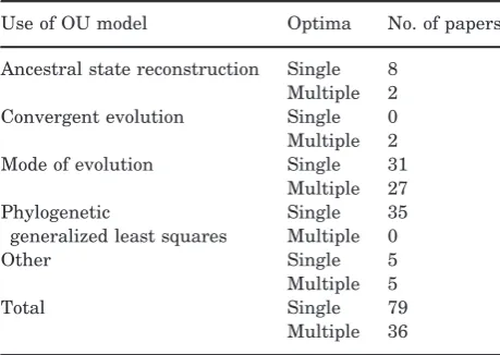
Table 1. The most common uses of Ornstein Uhlenbeck

models in ecology, evolutionary biology and palaeontology papers published between 2005 and 2013; see Supporting Information for details

Use of OU model Optima No. of papers

Ancestral state reconstruction Single 8 Multiple 2 Convergent evolution Single 0 Multiple 2 Mode of evolution Single 31

Multiple 27 Phylogenetic

generalized least squares

Single 35 Multiple 0

Other Single 5

Multiple 5

Total Single 79

In many implementations of the OU model (e.g. GEIGER; Harmon et al., 2008), lis the same as the state of the root at time zero,X(0). This is referred to as a ‘single stationary peak’ or SSP model (sensu Harmon et al., 2010). Some implementations also allow users to estimateX(0) (e.g. OUwie; Beaulieu & O’Meara, 2012). WhereX(0)6¼lthis is referred to as a single peak OU process. However, estimating X(0) can sometimes lead to nonsensical values of _l, i.e. far outside the range of values for the trait, so results should be interpreted with caution. X(0) can also be defined a priori, but this is only appropriate when fossil data, or other independent evidence, allow confident estimates of the root state.

When_ais close to zero, evolution is approximately Brownian (but note that in the special case of a sin-gle peak OU model with X(0)6¼l, when l is zero, evolution approximates Brownian motion with a trend; Hansen, 1997; Bensonet al., 2014), then as a gets larger the non-Brownian behaviour of the model starts to become apparent. Eventually, when _a is really large, all imprint of history is lost and the trait evolution is essentially a rapid burst at the pre-sent. Note that a scales with tree height (i.e. the maximum distance from the root of the tree to the tips); taller trees will have lower _a values, all else being equal, because there is more time for traits to return to the optimum value, and thus the strength of the pull towards the optimum, a, can be smaller. Thus,avalues need to be interpreted relative to tree height. Generally the simplest solution is to rescale tree heights to 1 (e.g. Ives & Garland, 2010; see sim-ulations below). Ives & Garland (2010) suggest inter-preting log (a) after rescaling trees to a height of 1, rather than rawa. They equate–log (a)=4 as a very low, almost Brownian, value and –log (_a)=4 as a very high value. Others (e.g. Hansen & Bartoszek, 2012; Slater, 2015) prefer to use the phylogenetic half-life:t1

2 (see ‘Recommendations for interpretinga’ below).

PERFORMANCE OF THE OU MODEL

To explore some issues with the OU model in more detail, we ran a number of simulations designed to mirror the use of OU models in the literature.

SIMULATING PHYLOGENIES AND DATA

We simulated phylogenies with 25, 50, 100, 150, 200, 500, or 1000 tips under pure birth, constant-rate Birth–Death (extinction fractions of 0.25, 0.5 and 0.75) or temporally varying speciation rate (specia-tion rate modelled as time from the root raised to the power 0.2, 0.5, 2 and 5) models. We simulated 1000

phylogenies for each combination of tips and models resulting in 56 000 simulated phylogenies in total. Trees were simulated using the R package TESS (Hohna, 2013). We then simulated the evolution of a single trait under a Brownian motion model on each phylogeny using the R package MOTMOT (Thomas & Freckleton, 2011). All our simulated trees and data are available on GitHub: https://github.com/ nhcooper123/OhYou.

PERFORMANCE OF

a

To determine whether a is biased under conditions where it should be zero, and whether Likelihood ratio tests are appropriate for use with the OU model, we estimated_afor each of our simulated phy-logenies and data, and compared the fit of a Brown-ian model with that of an OU model using a Likelihood ratio test with 1 degree of freedom with the transformPhylo.ML function in MOTMOT (Tho-mas & Freckleton, 2011; https://github.com/ ghthomas/motmot). This mirrors the common situa-tion where researchers fit Brownian and OU models and then use Likelihood ratio tests to select the ‘best’ model. We then estimated the rejection rate of the null (Brownian) model for each set of simulations. We refer to this measure as the Type I error rate for the OU model.

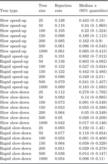
We find that Type I error rates are unacceptably high when tree size is small (Tables 2, 3), i.e. the OU model is often favoured, even though the Brownian model was used to generate the data. For some tree shapes, particularly where speciation rates acceler-ate towards the present, Type I error remains>0.05 even for trees with 1000 tips (Table 3). This shows that, in general, analyses based on small datasets are prone to biases that decrease only slowly as the size of the dataset increases. Unfortunately, OU models are often fitted to phylogenies with fewer than 100 taxa (mean=166.9743.86, median=58; Fig. 3; see Supporting Information). We provide rec-ommendations related to these findings below.

reference to the increasingly commonly used phylo-genetic half-life.

EFFECTS OF MEASUREMENT ERROR ONOUMODEL PERFORMANCE

Measurement error can strongly affect the results of comparative analyses (Silvestro et al., 2015), and appears to influence whether OU is the favoured model across a range of datasets (see Pennell et al., 2015). Therefore, we also investigated whether add-ing error to our simulated data influenced estimates of_a.

We used the same procedure as above to simulate trait data under a Brownian motion model with known error. Specifically, we simulated trees under

a Yule model with 25, 50, 100, 150, 200, 500 or 1000 tips and added branch length of (1) 1%, (2) 5% or (3) 10% of the tree height to the tips of the simulated trees. We then simulated data under a Brownian model on each tree. All our simulated trees and data are available on GitHub: https://github.com/nhcoop-er123/OhYou.

We compared the fit of a Brownian model with that of an OU model using Likelihood ratio tests as described above, using the original trees without the addition of extra branch length to the tip edges. Our expectation is that the OU model should fit the data better than the Brownian model because the _a parameter should account for much of the error. In this case, rejection of the Brownian model does not represent Type I error because it would be quite cor-rect to reject the Brownian model. However, the

Table 2. Rejection rate andaestimates for data simu-lated under a constant-rate Brownian model on a range of constant-rate birth death trees

Tree type Tree size Rejection rate

Mediana

(95% quantiles)

d/b=0 25 0.095 0.165 (0–1.498) d/b₌0 50 0.074 0.077 (0_–0.589) d/b=0 100 0.078 0.045 (0–0.343) d/b=0 150 0.057 0.034 (0–0.249) d/b=0 200 0.055 0.021 (0–0.199) d/b=0 500 0.045 0.012 (0–0.115) d/b₌0 1000 0.039 0.006 (0_–0.075) d/b=0.25 25 0.093 0.136 (0–0.968) d/b₌0.25 50 0.092 0.069 (0_–0.478) d/b=0.25 100 0.065 0.04 (0–0.267) d/b=0.25 150 0.065 0.031 (0–0.213) d/b=0.25 200 0.054 0.025 (0–0.166) d/b=0.25 500 0.047 0.01 (0–0.095) d/b=0.25 1000 0.044 0.005 (0–0.06) d/b=0.5 25 0.102 0.104 (0–0.851) d/b₌0.5 50 0.09 0.057 (0_–0.394) d/b=0.5 100 0.075 0.039 (0–0.219) d/b₌0.5 150 0.056 0.022 (0_–0.154) d/b=0.5 200 0.066 0.017 (0–0.138) d/b=0.5 500 0.047 0.009 (0–0.07) d/b=0.5 1000 0.045 0.004 (0–0.047) d/b=0.75 25 0.111 0.068 (0–0.572) d/b₌0.75 50 0.099 0.044 (0_–0.28) d/b=0.75 100 0.081 0.022 (0–0.146) d/b₌0.75 150 0.086 0.019 (0_–0.108) d/b=0.75 200 0.069 0.012 (0–0.088) d/b₌0.75 500 0.05 0.006 (0_–0.047) d/b=0.75 1000 0.045 0.003 (0–0.03)

Tree type refers to the extinction fraction for the birth– death trees. The rejection rate is the proportion of Orn-stein Uhlenbeck models favoured relative to a Brownian motion model.

Table 3. Rejection rate andaestimates for data simu-lated under a constant-rate Brownian model on trees sim-ulated under time-variable speciation rates

Tree type

Tree size

Rejection rate

Mediana

(95% quantiles)

Slow speed-up 25 0.126 0.443 (0–3.18) Slow speed-up 50 0.118 0.34 (0_–1.963) Slow speed-up 100 0.105 0.22 (0–1.324) Slow speed-up 150 0.098 0.189 (0–1.113) Slow speed-up 200 0.085 0.162 (0–0.9) Slow speed-up 500 0.061 0.096 (0–0.545) Slow speed-up 1000 0.061 0.065 (0_–0.415) Rapid speed-up 25 0.191 0.882 (0–7.012) Rapid speed-up 50 0.136 0.603 (0_–4.082) Rapid speed-up 100 0.122 0.527 (0–3.024) Rapid speed-up 150 0.122 0.442 (0–2.485) Rapid speed-up 200 0.086 0.349 (0–2.01) Rapid speed-up 500 0.079 0.241 (0–1.437) Rapid speed-up 1000 0.069 0.183 (0–1.083) Slow slow-down 25 0.112 0.278 (0–1.792) Slow slow-down 50 0.082 0.14 (0_–0.985) Slow slow-down 100 0.073 0.091 (0–0.549) Slow slow-down 150 0.053 0.055 (0_–0.388) Slow slow-down 200 0.064 0.05 (0–0.349) Slow slow-down 500 0.05 0.028 (0–0.209) Slow slow-down 1000 0.042 0.017 (0–0.146) Rapid slow-down 25 0.093 0.192 (0–1.45) Rapid slow-down 50 0.077 0.118 (0_–0.854) Rapid slow-down 100 0.058 0.061 (0–0.408) Rapid slow-down 150 0.064 0.038 (0_–0.329) Rapid slow-down 200 0.051 0.029 (0–0.278) Rapid slow-down 500 0.036 0.014 (0_–0.147) Rapid slow-down 1000 0.054 0.006 (0–0.11)

reason for the better fit would be entirely unrelated to any macroevolutionary process.

Table 4 shows the proportion of data sets in which the OU model is favoured over the Brownian model for data simulated under Brownian motion with error. The expectation is that the OU model should fit better because the branch length transformation partially captures the non-Brownian component (the error). There are two points worth noting. First, the frequency with which the OU model is favoured increases with tree size. With as little as 5% error, the OU model becomes extremely difficult to reject, even for trees with just 100 species. This is impor-tant for the interpretation of the OU model; we can-not conclude anything about the evolutionary process from a single optimum OU model unless error is ade-quately accounted for. Second, for moderate amounts of error (5–10%), estimates of a are consistently>1. Large values of a are similarly difficult to interpret because they are indicative that the signal of the past has been overwritten.

LIMITATIONS OF THE OU MODEL

Although it is possible to create and implement new models for comparative data that encompass a range of processes, we have to be aware that such models are statistically complex and may behave in unex-pected ways. Transformations of the variance– covari-ance matrix in the Brownian model (e.g. k; Pagel, 1997) are an attractive and computationally simple way to modify the basic model to include evolution-ary processes. But, as first pointed out by Grafen (1989), the statistical consequences of these modifica-tions can include biases and problems with interpre-tation. The results of our simulations illustrate that such problems can occur under conditions that clo-sely match the size and type of datasets that are commonly used (Fig. 3, Supporting Information, Table S1).

In the case of the OU model, there are several lim-itations worth highlighting:

1. Type I error rates are high when sample size is low. The results of the simulations indicate that, in general, analyses based on small datasets are prone to biases that decrease only slowly as the size of the dataset increases.

2. Likelihood ratio tests are untrustworthy. All Like-lihood ratio tests assume that the LikeLike-lihood ratio statistic is asymptotically (i.e. as sample sizes become large) _v2_{-distributed. In the OU}

model _ais bounded (i.e. it cannot be any smaller than zero) and has a non-linear effect on the expected variances, so the assumptions of the Likelihood ratio test are not likely to be upheld

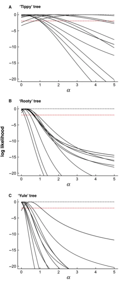
Figure 2. Examples of profile likelihoods for selected

for small samples. Our simulations indicate that Likelihood ratio tests should not be relied upon for analyses with small sample sizes, and that for robust inference and testing, alternatives, such as simulation and Monte Carlo Markov chains (MCMC), should be considered [see Recommenda-tions and potential soluRecommenda-tions (1) and (2) below]. Note that these issues will also apply when using the Akaike information criterion (AIC) to com-pare models, as this is essentially the same as performing a Likelihood ratio test. AIC also presents other difficulties when used for com-plex models such as those used in phylogenetic

comparative analyses, so we recommend avoiding them for these reasons.

3. Measurement error increases Type I error rates. Our results show that a simple Brownian process can be mistaken for an OU process when a small amount of error is added to the data. The effects of measurement error become more severe with increasing tree size. These limitations mean that when evidence for the OU model is found, the results should be interpreted with caution, partic-ularly where there is likely to be intraspecific variation or measurement error in the data.

RECOMMENDATIONS AND POTENTIAL SOLUTIONS

We have highlighted several issues with the OU model above. These can be broadly divided into two classes: (1) fitting the model and (2) interpreting model parameters. These issues can be at least par-tially addressed with additional or alternative ana-lytical approaches. Below we make recommendations for best practice in fitting the model and approaches to interpret model parameters. We highlight areas of future research that may be important in alleviating outstanding issues.

RECOMMENDATIONS FOR MODEL FITTING

1. Simulate under the null model. OU models should not be applied to small trees. Our simula-tions indicate that trees with > 200 tips are nec-essary to obtain acceptable Type I error rates. However, we are cautious about recommending a minimum tree size because the performance of the OU model may vary among datasets for

rea-Table 4. Rejection rate andaestimates for data simulated under a constant rate Brownian model with 0, 1, 5 or 10% measurement error (m.e.)

Tree size

Rejection rate Median_a(95% quantiles)

0% 1% 5% 10% 0% 1% 5% 10%

25 0.095 0.157 0.318 0.478 0.165 (0–1.498) 0.234 (0–1.507) 0.372 (0–5.51) 0.574 (0–20) 50 0.074 0.203 0.542 0.756 0.077 (0_–0.589) 0.163 (0_–0.789) 0.372 (0_–2.2) 0.538 (0.062_–14.381) 100 0.078 0.251 0.807 0.957 0.045 (0–0.343) 0.135 (0–0.503) 0.357 (0.06–1.236) 0.54 (0.153–4.094) 150 0.057 0.387 0.947 0.997 0.034 (0_–0.249) 0.14 (0_–0.445) 0.37 (0.121_–1.104) 0.566 (0.224_–7.381) 200 0.055 0.487 0.982 1 0.021 (0–0.199) 0.136 (0–0.411) 0.385 (0.142–1.089) 0.544 (0.257–2.98) 500 0.045 0.848 1 1 0.012 (0–0.115) 0.152 (0.035–0.344) 0.394 (0.219–0.919) 0.58 (0.319–3.729) 1000 0.039 0.995 1 1 0.006 (0–0.075) 0.168 (0.079–0.335) 0.417 (0.259–0.844) 0.596 (0.361–2.328)

The rejection rate is the proportion of Ornstein Uhlenbeck models favoured relative to a Brownian motion model.

Number of taxa

Number of papers

0 200 400 600 800

0 5 10 15 20 25 30

Figure 3. The number of taxa in phylogenies used to fit

sons other than tree size. We note also that large trees are particularly susceptible to issues arising from unaccounted measurement error in the data. Instead, we suggest using simulations to assess the model fit. Simulating data under the Brownian model will generate null distributions (e.g. Boettigeret al., 2012) and allow straightfor-ward assessment of model fit, for example by gen-erating appropriate critical values for Likelihood ratio tests. Boettiger et al.(2012) discuss this at length and other papers use similar approaches (e.g. Martins & Garland, 1991; Freckleton, Har-vey & Pagel, 2002).

2 Consider Bayesian approaches. An alternative but less explored approach is to use Bayesian meth-ods. Bayesian model fitting has not been widely available for OU model fitting until recently but is now possible in R packages including diversitree (FitzJohn, 2012) and GEIGER (the Single Station-ary Peak model in fitContinuousMCMC; Harmon et al., 2008) and stand-alone software including BayesTraits (Pagel & Meade, 2013).

We explored Bayesian methods as a possible rem-edy to the limitations of fitting OU models in a Likeli-hood framework. We repeated our simulations in a Bayesian framework implemented in BayesTraits (Pagel & Meade, 2013). We determined the fit to an OU model using Bayes factors estimated from a step-ping stone sampling procedure (Xieet al., 2010). The marginal likelihoods of the models were calculated using a stepping stone sampler in which 50 stones were drawn from a beta distribution witha=0.4 and b=1. Each stone was sampled for 20 000 iterations (with the first 5000 iterations discarded). We use stepping stone sampling as it has been shown to esti-mate the marginal likelihood better than the har-monic mean (Baele et al., 2012). We treated Bayes factors>2 as evidence favouring the OU model (Kass & Raftery, 1995). We ran the MCMCs for 19106 iterations, disregarding the first 19104_{as burn-in.}

Following burn-in the chains were sampled every 1000 iterations to ensure independence of each con-secutive sample. Multiple independent chains were run for each analysis to ensure convergence was reached. An important challenge for Bayesian approaches is selection of appropriate priors. We used three alternative sets of priors ona: (1) an exponen-tial distribution with mean=1, (2) an exponential distribution with mean=10 and (3) a uniform distri-bution bounded at 0 and 20. For all analyses we used a uniform100 to 100 prior for_land uniform 0–100 prior forr2.

Table 5 shows the results from the exponential prior with mean=10. This is a broad, liberal prior, but our results are similar regardless of priors. The

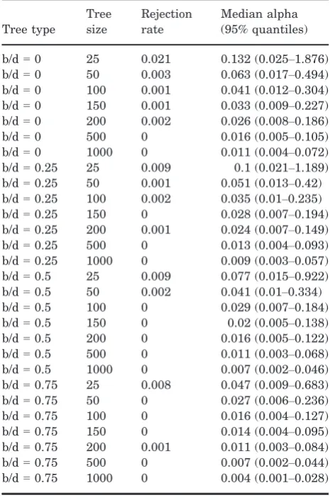
Bayesian approach results in highly conservative rejection rates regardless of tree shape in the absence of measurement error. While this is encouraging from the perspective of falsely rejecting the Brownian null model, it is also indicative of potentially low statistical power, although testing would be required to confirm this. The Bayesian approach also appears to more readily handle low levels of measurement error (Table 6). With 1% mea-surement error the Bayesian approach retains acceptable rejection rates (<0.05) for trees of up to 150 tips. However, more error or larger trees result in the frequent rejection of the Brownian model. As noted above, this is not an issue of Type I error and it is entirely correct that the Brownian model is

Table 5. Rejection rate andaestimates for data simu-lated under a constant-rate Brownian model on a range of constant-rate birth death trees using Bayesian methods

Tree type

Tree size

Rejection rate

Median alpha (95% quantiles)

b/d=0 25 0.021 0.132 (0.025–1.876) b/d₌0 50 0.003 0.063 (0.017_–0.494) b/d=0 100 0.001 0.041 (0.012–0.304) b/d=0 150 0.001 0.033 (0.009–0.227) b/d=0 200 0.002 0.026 (0.008–0.186) b/d=0 500 0 0.016 (0.005–0.105) b/d₌0 1000 0 0.011 (0.004_–0.072) b/d=0.25 25 0.009 0.1 (0.021–1.189) b/d₌0.25 50 0.001 0.051 (0.013_–0.42) b/d=0.25 100 0.002 0.035 (0.01–0.235) b/d=0.25 150 0 0.028 (0.007–0.194) b/d=0.25 200 0.001 0.024 (0.007–0.149) b/d=0.25 500 0 0.013 (0.004–0.093) b/d=0.25 1000 0 0.009 (0.003–0.057) b/d=0.5 25 0.009 0.077 (0.015–0.922) b/d₌0.5 50 0.002 0.041 (0.01_–0.334) b/d=0.5 100 0 0.029 (0.007–0.184) b/d₌0.5 150 0 0.02 (0.005_–0.138) b/d=0.5 200 0 0.016 (0.005–0.122) b/d=0.5 500 0 0.011 (0.003–0.068) b/d=0.5 1000 0 0.007 (0.002–0.046) b/d=0.75 25 0.008 0.047 (0.009–0.683) b/d₌0.75 50 0 0.027 (0.006_–0.236) b/d=0.75 100 0 0.016 (0.004–0.127) b/d₌0.75 150 0 0.014 (0.004_–0.095) b/d=0.75 200 0.001 0.011 (0.003–0.084) b/d₌0.75 500 0 0.007 (0.002_–0.044) b/d=0.75 1000 0 0.004 (0.001–0.028)

rejected. In such cases emphasis should shift to how thea parameter is interpreted. Bayesian analysis is a promising approach for OU model fitting. However, further testing of the Bayesian approach to simu-lated data sets under a wide range of values ofa is necessary to fully characterize performance.

RECOMMENDATIONS FOR INTERPRETING

a

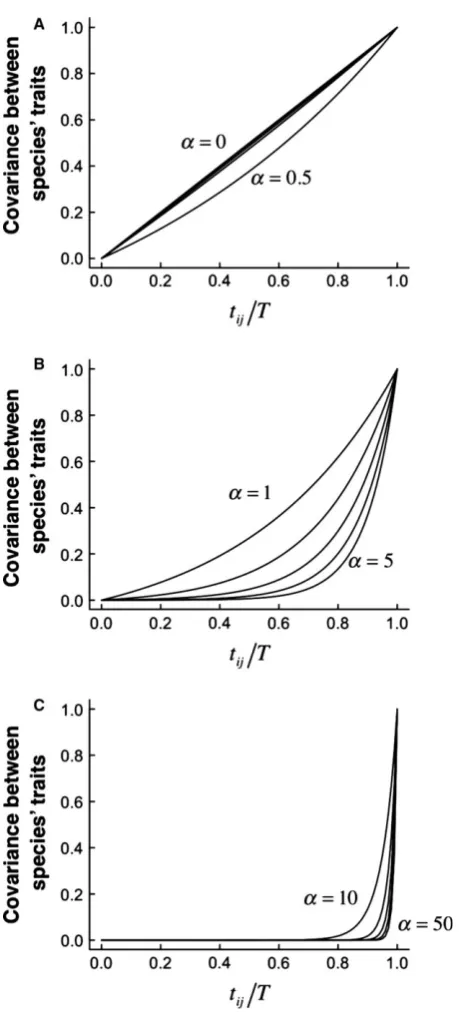
(1) Consider plausible alternative hypotheses. Because the OU model was proposed with evo-lutionary processes in mind, alternative and arguably more parsimonious explanations for favouring OU models and interpreting non-zero a are often overlooked. The effects of measure-ment error in particular suggest that a must always be interpreted with caution. Many issues of misinterpretation can be solved by carefully inspecting the _a parameter when an OU model is favoured. Often, when Likelihood ratio tests suggest the OU model should be favoured over the Brownian model, estimates of _a are actually very small and biologically indistinguishable from Brownian (e.g. examples in Harmon et al., 2010). In these circum-stances, it is likely that measurement error, intraspecific variation or phylogenetic uncer-tainty are generating noise that is more effec-tively modelled by the extra parameters in the OU model than by the Brownian model alone. Thus, this does not reflect any kind of OU pro-cess underlying the data. The similarity between Brownian and OU models with small a is demonstrated in Fig. 4. At the other extreme, as values of _a become larger, the effects of changing a on model predictions are increasingly small and large values of a are indistinguishable from white-noise.

One good strategy for data exploration would be to simulate data under Brownian and the favoured OU model to generate distributions of parameters under known values. These can then be compared with results for your dataset (see Slater, 2014; Slater & Pennell, 2014; for a related approach). This is impor-tant because we have shown that the shape of a phy-logeny has consequences for parameter biases and hypothesis tests. Any given tree will therefore gener-ate unique parameter estimgener-ates. Generating data under the favoured OU model will allow an assess-ment of whether it is possible to retrieve known val-ues, or whether there is evidence of bias.

(2) Calculate the phylogenetic half-life. Thea param-eter ranges from zero to infinity (although in practice an upper bound is often set; for example, in GEIGER this is_a=150; Harmonet al., 2008), thus recognizing ‘small’ or ‘large’ values may not be intuitive.acan sometimes be interpreted more easily by using it to estimate the ‘phylogenetic half-life’ (t1

2) of a trait, i.e. the time it takes for a species entering a new niche to evolve halfway toward its new expected optimum (Hansen, 1997), as follows:

t1 2¼

lnð2Þ a

If t1

2 is short relative to the branch lengths of the phylogeny, evolution towards the optimum trait value is fast, residual phylogenetic correlations are weak and there is little influence of the past on trait values (Hansen, 1997). t1

2 equal to the height of the phylogeny is a moderate value (Hansen & Bartoszek, 2012). We would not advise interpreting t1

2 as liter-ally being ‘the time it takes for a species entering a new niche to evolve halfway toward its new expected optimum’ (Hansen, 1997). However, ift1

2 is extremely

Table 6. Rejection rate andaestimates for data simulated under a constant rate Brownian model with 0, 1, 5, or 10% measurement error (m.e.) using Bayesian methods

Tree size

Rejection rate Median_a(95% quantiles)

0% 1% 5% 10% 0% 1% 5% 10%

25 0.021 0.031 0.109 0.191 0.132 (0.025–1.876) 0.158 (0.03–2.076) 0.286 (0.034–3.726) 0.509 (0.049–5.848) 50 0.003 0.018 0.158 0.332 0.063 (0.017_–0.494) 0.107 (0.019_–0.723) 0.315 (0.034_–2.245) 0.481 (0.057_–5.679) 100 0.001 0.033 0.364 0.708 0.041 (0.012–0.304) 0.11 (0.016–0.485) 0.333 (0.044–1.202) 0.521 (0.135–3.183) 150 0.001 0.045 0.637 0.906 0.033 (0.009_–0.227) 0.123 (0.016_–0.424) 0.357 (0.108_–1.074) 0.553 (0.208_–4.977) 200 0.002 0.097 0.819 0.978 0.026 (0.008–0.186) 0.126 (0.015–0.399) 0.372 (0.134–1.098) 0.538 (0.243–2.845) 500 0 0.426 1 1 0.016 (0.005–0.105) 0.147 (0.032–0.34) 0.391 (0.214–0.923) 0.575 (0.311–3.36) 1000 0 0.86 1 1 0.011 (0.004–0.072) 0.165 (0.077–0.335) 0.414 (0.256–0.85) 0.592 (0.359–2.278)

large relative to tree height, it suggests that if an OU process is acting, it is extremely weak (e.g. for a clade that is 50 Myr old, a t1

2 of 100 Myr suggests a species will not approach the optimum within the temporal range of the clade), and thus should not be interpreted as evidence of any kind of process. As a further note of caution, it is important to recognize that biases in the estimation ofawould lead to simi-lar biases int1

2.

(3) If possible, include ancillary data. If data on fos-sils are available then these could be incorpo-rated into the analysis (Slater, Harmon & Alfaro, 2012). Indeed, if fossil taxa can be reli-ably placed in the phylogeny then they may improve model accuracy and a strong case can be made that fossils should be included. On the other hand, if there is substantial uncertainty in fossil placement then they should be treated cau-tiously. Placement of fossil taxa is implemented in GEIGER (Harmon et al., 2008) and Bayes-Traits (Pagel & Meade, 2013). A caution here is that the OU model for non-ultrametric trees has to be carefully parameterized because for non-ultrametric trees the co-variances depend on both the shared distances between species and the distance of a node to the nearest tip (see eqn A6). This creates potential problems in parameterization and in interpretation because the variance–covariance matrix is no longer tree-like; for example, related species can effectively become more similar to one another than to themselves –an inherently non tree-like pattern (Slater, 2014). Some current implementations of the OU model are based on transforming the tree directly, rather than transforming the vari-ance–covariance matrix (e.g. MOTMOT; Thomas & Freckleton, 2011). These implementations should not be used with fossil data.

CONCLUSIONS AND OUTSTANDING ISSUES

A recurring theme from our simulations is that inter-pretation of OU models is not straightforward. More focus is needed on the interpretation ofarather than simply model fit. Even when the OU model is favoured,amay be so small as to be indistinguishable from Brownian motion in any biological sense. It would clearly be very useful to have estimates of mea-surement error for all species traits, although the inclusion of species-specific variances has to be done carefully (e.g. Grafen, 1989). Several approaches for accounting for error have been proposed and warrant wider implementation for OU models and other

models of trait evolution (e.g. Lynch, 1991; Martins & Hansen, 1997; Ives, Midford & Garland, 2007; Hansen & Bartoszek, 2012; Rohlfs, Harrigan & Nielsen, 2014), but it is outside our scope to explore these here.

Indeed, the problems that we report are not limited to OU models. Any model of trait evolution that attempts to account for non-Brownian components of trait variation is susceptible to being misled by mea-surement error, and in some scenarios meamea-surement error can also incorrectly favour Brownian motion over the true model, e.g. if the true model is Early Burst. The fundamental problem is that rejection of the Brownian model in favour of another model does not necessarily say anything about process. This prob-lem can be alleviated to some extent if model compar-isons are set in a firm hypothesis-testing framework in which alternative hypotheses make clear predic-tions of emerging patterns that can be unambiguously associated with particular models (e.g. Cooper, Freck-leton & Jetz, 2011), although this does not appear to be possible for comparisons of the single stationary peak OU model with noisy Brownian processes. We should therefore not use any statistical model without thinking carefully about the limits in terms of both data and interpretation.

EPILOGUE: THE CHALLENGES OF OPEN AND REPRODUCIBLE SCIENCE

At the symposium that generated this special issue, one of us (N.C.) gave a talk on Open Science and reproducibility. We have therefore tried to make this paper as open and reproducible as possible. All simu-lated phylogenies, data and R code are available on GitHub: https://github.com/nhcooper123/OhYou. How-ever, although our R code is provided, it is disorga-nized and thus difficult to use. We also do not provide an automated way of reproducing the data collection for our literature review. Nor do we use tools such as Travis CI (travis-ci.org), Docker (www.docker.com) or packrat (Ushey et al., 2015) to increase the repro-ducibility of our analyses. Additionally, we use Bayes-Traits to run our Bayesian analyses. BayesBayes-Traits is free to download as a binary executable for various platforms but it is not Open Source. This means that while BayesTraits analyses are reproducible, the soft-ware has limitations with respect to long-term devel-opment of the code. We included this epilogue to highlight that fully reproducible and Open Science is challenging, but we are trying to improve. With a little effort most people should be able to produce something vaguely reproducible, and to provide their data and code, moving us all slightly closer to truly reproducible and Open Science.

ACKNOWLEDGEMENTS

Thanks to Rich FitzJohn, Mark Pagel and Matt Pen-nell for fruitful discussions about OU models, and four anonymous reviewers and Graham Slater for helpful comments on previous versions of the manu-script. N.C. was supported by The European Com-mission CORDIS Seventh Framework Program (FP7) Marie Curie CIG grant, proposal number: 321696. G.H.T. was supported by a Royal Society University Research Fellowship, grant number: UF120016. C.V. was supported by a Leverhulme Trust Research Pro-ject Grant RPG-2013-185. A.M. was supported by BBSRC grant BB/K004344/1 and the computing time was funded by European Research Council Grant no. 268744, ‘MotherTongue’.

This paper was a contribution to a Linnean Society symposium on “Radiation and Extinction: Investigat-ing Clade Dynamics in Deep Time” held on Novem-ber 10–11, 2014 at the Linnean Society of London and Imperial College London and organised by Anjali Goswami, Philip D. Mannion, and Michael J. Benton, the proceedings of which have been collated as a Special Issue of the Journal.

REFERENCES

Baele G, Lemey P, Bedford T, Rambaut A, Suchard MA,

Alekseyenko AV. 2012.Improving the accuracy of

demo-graphic and molecular clock model comparison while accom-modating phylogenetic uncertainty.Molecular Biology and Evolution29:2157_–2167.

Beaulieu JM, O’Meara B, 2012. OUwie: analysis of

evolutionary rates in an OU framework. R package version 1.

Beaulieu JM, Jhwueng DC, Boettiger C, O’Meara BC.

2012. Modeling stabilizing selection: expanding the

Orn-stein–Uhlenbeck model of adaptive evolution.Evolution66: 2369_–2383.

Benson RB, Frigot RA, Goswami A, Andres B, Butler

RJ. 2014.Competition and constraint drove Cope’s rule in

the evolution of giant flying reptiles. Nature Communica-tions5:3567.

Blackburn DC, Siler CD, Diesmos AC, McGuire JA,

Cannatella DC, Brown RM. 2013.An adaptive radiation

of frogs in a Southeast Asian island archipelago.Evolution 67:2631–2646.

Blankers T, Adams D, Wiens J. 2012.Ecological radiation

with limited morphological diversification in salamanders. Journal of Evolutionary Biology25:634_–646.

Blomberg S, Garland T, Ives AR. 2003.Testing for

phylo-genetic signal in comparative data: behavioral traits are more labile.Evolution57:717_–745.

Boettiger C, Coop G, Ralph P. 2012. Is your phylogeny

Butler MA, King A. 2004.Phylogenetic comparative analy-sis: a modelling approach for adaptive evolution.The Amer-ican Naturalist164:683–695.

Cardillo M. 2015.Geographic range shifts do not erase the

historic signal of speciation in mammals. The American Naturalist185:343_–353.

Cavalli-Sforza LL, Edwards AWF. 1967. Phylogenetic

analysis. Models and estimation procedures. American Journal of Human Genetics19:233_–257.

Christin PA, Osborne CP, Chatelet DS, Columbus JT, Besnard G, Hodkinson TR, Garrison LM, Vorontsova

MS, Edwards EJ. 2013.Anatomical enablers and the

evo-lution of C4 photosynthesis in grasses. Proceedings of the National Academy of Sciences USA110:1381–1386.

Cooper N, Purvis A. 2010.Body size evolution in mammals:

complexity in tempo and mode. The American Naturalist

175:727–738.

Cooper N, Freckleton RP, Jetz W. 2011.Phylogenetic

con-servatism of environmental niches in mammals. Proceed-ings of the Royal Society of London Series B: Biological Sciences278:2384–2391.

Felsenstein J. 1973.Maximum-likelihood estimation of

evo-lutionary trees from continuous characters.American Jour-nal of Human Genetics25:471–492.

FitzJohn RG. 2012. diversitree: comparative phylogenetic

analyses of diversification in R. Methods in Ecology and Evolution3:1084_–1092.

Freckleton R. 2009.The seven deadly sins of comparative

analysis.Journal of Evolutionary Biology22:1367_–1375.

Freckleton RP, Harvey PH. 2006.Detecting non-Brownian

trait evolution in adaptive radiations. PLoS Biology 4: e373.

Freckleton R, Cooper N, Jetz W. 2011.Comparative

meth-ods as a statistical fix: the dangers of ignoring an evolution-ary model.The American Naturalist178:E10–E17.

Freckleton R, Harvey P, Pagel M. 2002. Phylogenetic

analysis and comparative data: a test and review of evi-dence.The American Naturalist160:712–726.

Grafen A. 1989. The phylogenetic regression. Philosophical

Transactions of the Royal Society of London Series B: Bio-logical Sciences326:119_–157.

Hansen TF. 1997.Stabilizing selection and the comparative

analysis of adaptation.Evolution51:1341_–1351.

Hansen TF, 2012.Adaptive landscapes and

macroevolution-ary dynamics. In: Svensson EI, Calsbeek R, eds.The adap-tive landscape in evolutionary biology. Oxford: Oxford University Press, 205–226.

Hansen TF, Bartoszek K. 2012.Interpreting the

evolution-ary regression: the interplay between observational and bio-logical errors in phylogenetic comparative studies. Systematic Biology61:413–425.

Harmon LJ, Weir JT, Brock CD, Glor RE, Challenger

W. 2008. GEIGER: investigating evolutionary radiations.

Bioinformatics24:129_–131.

Harmon L, Losos J, Davies TJ, Gillespie R, Gittleman J, Jennings BW, Kozak K, McPeek M, Moreno RF,

Near T. 2010.Early bursts of body size and shape

evolu-tion are rare in comparative data.Evolution64:2385–2396.

Harvey PH, Rambaut A. 2000. Comparative analyses for

adaptive radiations.Philosophical Transactions of the Royal Society of London Series B: Biological Sciences355:1599– 1605.

Ho LST, Ane C. 2013.Asymptotic theory with hierarchical

autocorrelation: Ornstein_–Uhlenbeck tree models. The Annals of Statistics41:957_–981.

Ho LST, Ane C. 2014.Intrinsic inference difficulties for trait

evolution with Ornstein_–Uhlenbeck models. Methods in Ecology and Evolution5:1133–1146.

Hohna S. 2013.Fast simulation of reconstructed phylogenies

under global time-dependent birth–death processes. Bioin-formatics29:1367_–1374.

Ingram T, Mahler DL. 2013.SURFACE: detecting

conver-gent evolution from comparative data by fitting Ornstein– Uhlenbeck models with stepwise Akaike Information Crite-rion.Methods in Ecology and Evolution4:416–425.

Ives AR, Garland T. 2010.Phylogenetic logistic regression

for binary dependent variables.Systematic Biology59:9–26.

Ives AR, Midford PE, Garland T. 2007. Within-species

variation and measurement error in phylogenetic compara-tive methods.Systematic Biology56:252_–270.

Kass RE, Raftery AE. 1995.Bayes factors. Journal of the

American Statistical Association90:773–795.

Lande R. 1976.Natural-selection and random genetic drift

in phenotypic evolution.Evolution30:314–334.

Lynch M. 1991. Methods for the analysis of comparative

data in evolutionary biology.Evolution45:1065–1080.

Martins EP. 1999.Estimation of ancestral states of

continu-ous characters: a computer simulation study. Systematic Biology48:642–650.

Martins EP, Garland T. 1991.Phylogenetic analyses of the

correlated evolution of continuous characters: a simulation study.Evolution45:534_–557.

Martins EP, Hansen TF. 1997.Phylogenies and the

com-parative method: a general approach to incorporating phy-logenetic information into the analysis of interspecific data. The American Naturalist149:646–667.

Nunn CL. 2011.The comparative approach in evolutionary

anthropology and biology. Chicago: University of Chicago Press.

O’Meara BC. 2012. Evolutionary inferences from

phyloge-nies: a review of methods.Annual Review of Ecology, Evo-lution and Systematics43:267–285.

Pagel M. 1997.Inferring evolutionary processes from

phylo-genies.Zoologica Scripta26:331–348.

Pagel M. 1999.Inferring the historical patterns of biological

evolution.Nature401:877_–884.

Pagel M, Meade A, 2013. BayesTraits v. 2.0. Reading:

University of Reading.

Pennell MW, Harmon LJ. 2013. An integrative view of

phylogenetic comparative methods: connections to popula-tion genetics, community ecology, and paleobiology.Annals of the New York Academy of Sciences1289:90_–105. Pennell MW, FitzJohn RG, Cornwell WK, Harmon LJ,

2015. Model adequacy and the macroevolution of

Pienaar J, Ilany A, Geffen E, Yom-Tov Y. 2013. Macroevolution of life-history traits in passerine birds: adaptation and phylogenetic inertia. Ecology Letters 16: 571_–576.

Price T. 1997. Correlated evolution and independent

con-trasts. Philosophical Transactions of the Royal Society of London Series B: Biological Sciences352:519_–529.

Quintero I, Wiens JJ. 2013. Rates of projected climate

change dramatically exceed past rates of climatic niche evo-lution among vertebrate species.Ecology Letters 16:1095– 1103.

Revell LJ. 2010. Phylogenetic signal and linear regression

on species data.Methods in Ecology and Evolution1: 319_– 329.

Rohlfs RV, Harrigan P, Nielsen R. 2014.Modeling gene

expression evolution with an extended Ornstein_–Uhlenbeck process accounting for within-species variation. Molecular Biology and Evolution31:201_–211.

Silvestro D, Kostikova A, Litsios G, Pearman PB,

Sala-min N. 2015.Measurement errors should always be

incor-porated in phylogenetic comparative analysis. Methods in Ecology and Evolution6:340_–346.

Slater GJ. 2014.Correction to ‘Phylogenetic evidence for a

shift in the mode of mammalian body size evolution at the Cretaceous_–Palaeogene boundary’, and a note on fitting macroevolutionary models to comparative paleontological data sets.Methods in Ecology and Evolution5:714_–718.

Slater GJ. 2015.Iterative adaptive radiations of fossil canids

show no evidence for diversity-dependent trait evolution.

Proceedings of the National Academy of Sciences USA112: 4897_–4902.

Slater GJ, Pennell MW. 2014. Robust regression and

posterior predictive simulation increase power to detect early bursts of trait evolution. Systematic Biology 63: 293_–308.

Slater GJ, Harmon LJ, Alfaro ME. 2012.Integrating

fos-sils with molecular phylogenies improves inference of trait evolution.Evolution66:3931_–3944.

Thomas GH, Freckleton RP. 2011. MOTMOT: models of

trait macroevolution on trees.Methods in Ecology and Evo-lution3:145–151.

Ushey K, McPherson J, Cheng J, Allaire J. 2015.

pack-rat: A dependency management system for projects and their R package dependencies. R package version: 3.

Uyeda JC, Harmon LJ. 2014.A novel Bayesian method for

inferring and interpreting the dynamics of adaptive land-scapes from phylogenetic comparative data. Systematic Biology63:902–918.

Wiens JJ, Ackerly DD, Allen AP, Anacker BL, Buckley LB, Cornell HV, Damschen EI, Davies TJ, Grytnes JA, Harrison SP, Hawkins BA, Holt RD, McCain CM,

Ste-phens PR. 2010.Niche conservatism as an emerging

prin-ciple in ecology and conservation biology. Ecology Letters 13:1310_–1324.

Xie W, Lewis PO, Fan Y, Kuo L, Chen MH. 2010.

Improv-ing marginal likelihood estimation for Bayesian phyloge-netic model selection.Systematic Biology60:150–160.

SUPPORTING INFORMATION

Additional Supporting Information may be found online in the supporting information tab for this article:

Table S1.Details of the papers used in our literature review.

APPENDIX

According to the Brownian model, a traitXevolves at random at a rater:

dXðtÞ ¼_rdWðtÞ ðA1Þ

whereW(t) is a white-noise function and is a random variate drawn from a normal distribution with mean 0 and variance r2. This model assumes that there is no overall drift in the direction of evolution [hence the expectation ofW(t) is zero] and that the rate of evolution is constant. The model has two parameters, _r and the state of the root at time zero,X(0). The Brownian model predicts after a timeTthe variance in trait value Xifor speciesiis:

varðXiÞ ¼r2T ðA2Þ

and the covariance in traits for speciesiandjis:

covðXi;XjÞ ¼r2tij ðA3Þ

variances accrue as a linear function of time.The OU model describes a mean-reverting process and has the following form, adding an extra term to the Brownian model:

dXðtÞ ¼ aðXðtÞ lÞ þrdWðtÞ ðA4Þ

The parameter l is a long-term mean, and it is assumed that species evolve around this value. r is the strength of evolutionary force that returns traits back towards the mean if they evolve away. This model has two parameters in addition to those of the Brownian model,aandl. The OU model predicts that after a time Tfor a speciesi, the variance in trait valueXiis:

varðXiÞ ¼r

2

2a1e

2aT _ðA5Þ

And for a pair of speciesiandj, the covariance in traits is:

covðXi;XjÞ ¼r

2

2_ae

2aðTtijÞð_1e2atijÞ ð_A6Þ

The variances and covariances predicted by eqns A5 and A6 are more complex than those predicted by the Brownian model. In the light of the results above, some properties of this model are worth highlighting:

(1) If a is small then evolution is approximately Brownian: if a is small then % 1 -e-2aT_{2aT, i.e. traits} accrue variance as if evolving according to a Brownian process.

(2) If speciesiandj diverged recently, evolution is approximately Brownian: if two species diverged recently, then T -tij0 and hence covðXi;XjÞ 1e2atij 2atij. Thus, recently diverged species provide little information relevant to estimating non-Brownian evolution according to an OU process.