This is a repository copy of From LATE to MTE : Alternative methods for the evaluation of policy interventions.
White Rose Research Online URL for this paper: http://eprints.whiterose.ac.uk/102312/
Version: Accepted Version Article:
Cornelissen, Thomas orcid.org/0000-0001-8259-5105, Dustmann, Christian, Raute, Anna et al. (1 more author) (2016) From LATE to MTE : Alternative methods for the evaluation of policy interventions. Labour Economics. pp. 47-60. ISSN 0927-5371
https://doi.org/10.1016/j.labeco.2016.06.004
[email protected] https://eprints.whiterose.ac.uk/ Reuse
Items deposited in White Rose Research Online are protected by copyright, with all rights reserved unless indicated otherwise. They may be downloaded and/or printed for private study, or other acts as permitted by national copyright laws. The publisher or other rights holders may allow further reproduction and re-use of the full text version. This is indicated by the licence information on the White Rose Research Online record for the item.
Takedown
If you consider content in White Rose Research Online to be in breach of UK law, please notify us by
1
F
ROM
LATE
TO
MTE:
A
LTERNATIVE
M
ETHODS FOR
THE
E
VALUATION OF
P
OLICY
I
NTERVENTIONS
1Thomas Cornelissen
Christian Dustmann
Anna Raute
Uta Schönberg
This version: June 2015
Abstract: This paper provides an introduction into the estimation of Marginal Treatment
Effects (MTE). Compared to the existing surveys on the subject, our paper is less technical and speaks to the applied economist with a solid basic understanding of econometric techniques who would like to use MTE estimation. Our framework of analysis is a generalized Roy model based on the potential outcomes framework, within which we define different treatment effects of interest, and review the well-known case of IV estimation with a discrete instrument resulting in a local average treatment effect (LATE). Turning to IV estimation with a continuous instrument we demonstrate that the 2SLS estimator may be viewed as a weighted average of LATEs, and discuss MTE estimation as an alternative and more informative way of exploiting a continuous instrument. We clarify the assumptions underlying the MTE framework, its relation to the correlated random coefficients model, and illustrate how the MTE estimation is implemented in practice.
JEL: C26, I26
Keywords: marginal treatment effects, instrumental variables, heterogeneous effects
1 Correspondence: Thomas Cornelissen, Department of Economics, University of York, Heslington, York
YO10 5DD, United Kingdom (email: [email protected]); Christian Dustmann, Department of Economics, University College London and CReAM, 30 Gordon Street, London WC1H 0AX, United Kingdom (email: [email protected]); Anna Raute, Department of Economics, University of Mannheim, L7, 3-5, 68161 Mannheim, Germany (email: [email protected]); Uta Schönberg, Department of Economics, University College London, CReAM and IAB, 30 Gordon Street, London WC1H 0AX, United Kingdom (email:
2
1 Introduction
Evaluating the causal effects of programs or policy interventions is a central task in empirical microeconomics. A common case is when the program under evaluation takes the form of a binary treatment, such as attending college or attending preschool. Responses to such treatments (and thus the treatment effect) will most likely differ across individuals. For example, more able individuals are likely to have lower costs of learning than low ability individuals and may therefore enjoy larger returns from college attendance. Children from disadvantaged backgrounds may benefit more from the exposure to a high quality child care program than children from advantaged backgrounds.
Even though treatment effects are likely to be heterogeneous, early standard econometric textbooks aimed at applied researchers did not pay much attention to heterogeneous treatment effects (see e.g. the textbooks by Johnston, 1963 or Maddala, 1992). Switching regression models, in which the effects of observed and unobserved characteristics are allowed to differ across states (where the state could be a treatment, and thus the treatment effect would depend on observed and unobserved characteristics) present early approaches of modelling treatment
effect heterogeneity and date back to the 1970’s (see Quandt, 1972; Heckman, 1976; and Lee,
1979). Rubin (1974) defines heterogeneous causal effects at the individual level in terms of
potential outcomes and discusses the average treatment effect (ATE) (or “average causal effect”) as an interesting parameter in order learn about the “typical” causal effect in a
3
problem of endogeneity caused by self-selection into treatment based on unobserved characteristics.
The “LATE revolution” in the 1990s changed the focus to identification of models when treatment effects are heterogeneous.2 The early papers in this literature by Imbens and Angrist (1994) and Angrist, Imbens and Rubin (1996) raised awareness about potential heterogeneity in returns and clarified the interpretation of IV estimates when treatment effects are heterogeneous. Heckman and Vytlacil (1998), Card (2001), and others proposed a control function approach based on the correlated random coefficient model as an alternative to conventional linear IV estimation which, under stronger assumptions than IV estimation, allows estimation of the ATE and yields some insight into the pattern of selection in the unobservables. The concept of the marginal treatment effect MTE was first introduced by Björklund and Moffitt (1987) in the context of a multivariate-normal switching regression model, in which they defined the “marginal gain” as the gain from treatment for individuals who are shifted into (or out of) treatment by a marginal change in the cost of treatment (i.e., the instrument). It was extended in a series of papers by Heckman and Vytlacil (1999, 2001b, 2005, 2007) who define the MTE as the gain from treatment for individuals shifted into (or out of) treatment by a marginal change in the propensity score (i.e., the predicted probability of treatment, which is a function of the instrument), develop non-parametric estimation methods, and clarify the connection of the switching regime self-selection model and of MTE with IV and LATE.
Since then the applied literature estimating MTE’s has been growing and now includes, in addition to many applications in the economics of education, applications as varied as the effect of foster care on child outcomes (Doyle, 2007), the effect of Disability Insurance receipt on labor supply (Maestas, Mullen, and Strand, 2013; French and Song, 2014) and the
2 In their 1994 Econometrica paper, Imbens and Angrist (1994) define the local average treatment effect
4
interaction of quantity and quality of children (Brinch, Mogstad, and Wiswall, 2015).3 Some recent surveys provide insightful discussions about MTE, see for example Blundell and Costa Dias (2009) who discuss MTE among a range of alternative policy evaluation approaches, French and Taber (2011) who discuss treatment effects and MTE and its relation to the Roy model, and the excellent, comprehensive, but technical treatments of MTE in Heckman and Vytlacil (2007) and Heckman, Urzúa and Vytlacil (2006), based on the earlier work by Heckman and Vytlacil (1999, 2001a, 2001b, 2005).
Drawing on these earlier papers, we provide here an introduction to the MTE framework, clarifying the discussion based on examples and developing it in a way that we believe is accessible to the applied economist. We commence by proposing a simple framework that allows for treatment heterogeneity, and define within this framework different treatment effects of interest such as the average treatment effect (ATE) the average treatment effect on the treated (ATT), and the average treatment effect on the untreated (ATU). We next discuss the well-known local average treatment effect (LATE) identified by IV with a binary instrument, before reviewing IV estimation with continuous instruments. We carefully describe how conventional ways of exploiting continuous instruments identify one overall IV effect that can be difficult to interpret and can hide interesting patterns of treatment effect heterogeneity. Based on the example of the correlated random coefficients model, we then discuss the control function approach as an alternative to conventional linear IV estimation. We explain that, under considerably stronger assumptions than conventional IV estimation, the control function estimator of that model identifies a more general effect than IV and reveals some information on the pattern of selection based on unobserved gains. After that, we turn to MTE estimation as a more informative way of exploiting a continuous instrument, which aims at identifying a
3 Applications in economics of education range from estimating the effects of child care attendance on child
5
continuum of treatment effects along the distribution of the individual unobserved characteristic that drives treatment decisions and allows the identification of a variety of treatment parameters such as ATE, ATT and ATU under potentially no stronger assumptions than IV estimation. We finally illustrate MTE estimation using two examples from the literature.
Our paper is less technical (and therefore also less rigorous) than the previous methodological contributions on MTE. It is written for the applied economist and introduces the method in a simple way, with a strong focus of relating MTE to more conventional IV estimation. The two applications we discuss illustrate to the applied researcher how MTE estimation can be implemented, and which additional insights hidden by IV estimation can be gained from MTE estimation.
2 Instrumental variables estimation with heterogeneous treatment effects
2.1 Framework of analysis and definition of treatment effects
Our general framework is a generalized Roy model based on the potential outcomes model and a latent variable discrete choice model for selection into treatment, as in Heckman and Vytlacil (1999) and most of the subsequent MTE literature.4 We assume that treatment is a binary variable denoted by . Let be an individual’s outcome under the hypothetical scenario that the individual is treated ( ), and the outcome under the hypothetical scenario that the individual is not treated ( ). For example, and could be an
individual’s wage in the two hypothetical scenarios that the individual attends college and does
not attend college, respectively. We model these potential outcomes as
Y X U (1)
Y X U (2)
4The potential outcome model, often also referred to as the “Rubin causal model” is a building block for the
6
where is the conditional mean of given in treatment state and captures
deviations from that mean implying that .5
Consider the following latent variable discrete choice model for selection into treatment, which forms the basis for the MTE approach:
(3)
if otherwise, (4)
where is the latent propensity to take the treatment. is interpretable as the net gain from treatment (because individuals take the treatment if ). The observed variables that affect the treatment decision include the same covariates as the outcome equations (1) and (2), and one or more variables excluded from the outcome equation. is an i.i.d. error term indicating unobserved heterogeneity in the propensity for treatment. Because the error term enters the selection equation with a negative sign, it embodies unobserved characteristics that make individuals less likely to receive treatment. One could thus label unobserved
“resistance” or “distaste” for treatment. The condition of taking the treatment can be
rewritten as . If we apply the c.d.f. of to this inequality, we get F F . Both sides of this inequality are now bounded within the
0/1-interval. The left-hand side represents the propensity score, the probability of being treated
based on the observed characteristics, and we refer to this term as F . The right-hand side, F , represents the quantiles of the distribution of the unobserved distaste for treatment , which we denote by U F . The treatment decision can thus be rewritten as
if U otherwise (5)
Individuals take the treatment if the propensity score exceeds the quantile of the distribution of at which the individual is located—that is, if the “encouragement” for treatment based on the observables and exceeds the unobserved distaste for treatment.
5
7
It should be noted that the two potential outcomes and are never jointly observed for the same individual. Instead, we observe the realized outcome which is equal to either or
depending on treatment status:
This is in essence the switching regression model of Quandt (1972) and Lee (1979). Substituting in for and shows that the potential outcome framework can be represented as the regression model
(6)
in which the coefficient on the treatment dummy varies across individuals and is equal to
This treatment effect has two components: The average gain of someone with given observed characteristics, , and an idiosyncratic individual-specific gain,
( ).
There are good reasons to expect treatment effect heterogeneity. Consider the example of college education. First, individuals can be heterogeneous in their untreated outcome ( ) reflecting differences in their experiences before entering college, such as the quality of their high-school education, family background, etc. If the main effect of college attendance is to equalize preexisting differences and to bring everyone to the same level, then would be more homogeneous than , and individuals with lower outcomes in the untreated state would have higher treatment effects. Alternatively, it could be that some individuals are more able to benefit from college attendance (maybe because their ability to learn is higher) so that they would have a higher even if was similar to that of other individuals. A higher for a given could also result from variation in the quality of the treatment, for example because colleges differ in the quality of their teaching and resources.
8
Consider for example the average treatment effect (ATE), the average treatment effect on the treated (ATT) and the average treatment effect on the untreated (ATU).6 Conditional on
they are defined as:
Conditional on , the ATE is the average treatment effect for an individual with given observed characteristics , while the ATT is the average treatment effect in the subgroup of the population that participates in the treatment conditional on Similarly, the ATU is the average treatment effect in the subgroup of the population that does not participate in the treatment conditional on . measures how individuals with observed characteristics would benefit on average from the treatment if everybody with these observed characteristics were participating in the treatment, or the expected effect if some individuals from the group of individuals with observed characteristics were randomly assigned to treatment. measures how those individuals with observed characteristics that are currently enrolled in the treatment benefit from it on average. on the other hand answers the question how those individuals with observed characteristics
who are currently not enrolled would benefit on average from treatment if they participated. By averaging these parameters over the appropriate distribution of , they can also be defined unconditionally:
(7) (8) (9)
6 For an extension of the framework including additional parameters on the cost and the surplus of the
9
In a linear specification for the conditional mean, that is, , the terms
, and would
simplify to , , and , respectively.
Sometimes we would like to know the aggregate effect of a specific policy change. This is given by the policy-relevant treatment effect (PRTE), see Heckman and Vytlacil (2001a, 2005) and Carneiro, Heckman, and Vytlacil (2011). Consider a policy change that affects the propensity score , but not potential outcomes ( or the unobservables of the selection process ). Such a policy will not change the underlying distribution of treatment effects, or preferences for treatment, but by changing the propensity score, the policy will change who selects into treatment based on the selection equation (5). Suppose is the treatment choice under the baseline policy, and is the treatment choice under the alternative policy. The PRTE conditional on is defined as (see Appendix A for details):
alternative policy baseline policy alternative policy baseline policy
and the corresponding unconditional effect is
(10)
The PRTE is the mean effect of going from a baseline policy to an alternative policy per net person shifted. It also corresponds to a weighted difference between the ATT under the alternative policy and the ATT under the baseline policy.7
7 If a policy only shifts additional people into treatment without shifting anyone out of the treatment, the
10
It is important to note that ATE, ATT, ATU and PRTE would be the same if there was no selection into treatment based on gains—one might imagine that individuals simply do not know their idiosyncratic returns to treatment or simply do not act on them. In reality it however seems likely that, depending on the context, individuals do select into treatment either directly based on gains, or based on characteristics that are related to gains. In consequence, the treatment parameters would in general differ. In the case of college attendance, for example, we would expect individuals who expect higher gains (e.g., higher future wages) from college attendance to be more likely to attend college. Such positive selection on gains is likely to occur based on both observed and unobserved characteristics. Positive selection on
‘unobserved gains’ implies that is positively related to conditional on , such that
and , and thus
. Positive selection on ‘observed gains’ implies that is positively related to , and thus ATT>ATE>ATU (provided that
).
When treatment effects are heterogeneous, it is of primary relevance to spell out which effect a given econometric method identifies. Next, we discuss which parameters linear instrumental variables estimation with a binary instrument and with a continuous instrument identify (Sections 2.2 and 2.3) and contrast these approaches with the control function estimator of the correlated random coefficient model (Section 2.4).
2.2 IV with a binary instrument and LATE
We first apply the IV estimator within subsamples stratified by , leading to covariate-specific IV estimates, similar to the covariate-specific treatment effects defined in section 2.1 above. We then derive one aggregate IV estimator representing an average across values of .
11
2.2.1 Covariate-Specific IV
Let be a binary instrumental variable. The IV estimator with binary instrument conditional on is equal to the Wald estimator
Wald (11)
In the sample of individuals with , this estimator divides the average difference in the outcome between individuals with the instrument switched on ( ) and individuals with the instrument switched off ( ) by the same difference in average treatment status.
The numerator is also commonly referred to as the ‘reduced form’ and the denominator as the
‘first stage’.
The assumptions under which this ratio estimates a causal effect are well understood and we state them only briefly here (see e.g. Angrist and Pischke, 2009 for a detailed discussion). Let denote the potential treatment state of individual i if and the potential treatment state of individual i if , so that observed treatment is equal to 8
The following assumptions are required for a causal interpretation of (11):
(i) Independence: | . This assumption first states that the instrument must be as good as randomly assigned conditional on . Random assignment ensures that the reduced-form effect of on has a causal interpretation (conditional on . The independence assumption further states that conditional on the instrument must affect potential outcomes only through its effect on the treatment probability —which is commonly referred to as the exclusion restriction.9 The exclusion restriction is necessary for the Wald estimator
8
Note that potential outcomes are indexed against the treatment state, whereas the potential treatment decision is indexed against the value of the instrument.
9 To make the distinction between random assignment and exclusion more explicit, Angrist and Pischke
12
to identify the causal effect of treatment on It should be noted that the exclusion restriction would be violated if treatment effects depended on the instrument.10 Within the Generalized Roy Model of equations (1)-(4), the independence assumption may be alternatively written as .
(ii) Existence of a first stage:
(iii) Monotonicity (or uniformity): or . This assumption means that all individuals who change their treatment status as a result of a change in the instrument either get all shifted into treatment, or get all shifted out of treatment.11 Here we assume that is coded in a way that provides an extra encouragement for treatment compared to , implying that monotonicity holds in the form of .
Under these assumptions the IV estimator in equation (11) above with a binary instrument applied in a subsample in which the covariates are fixed at identifies the covariate-specific Local Average Treatment Effect (LATE) defined by
LATE
(12)
then be written as | while the exclusion restriction may be written as
10 To see this, consider the following simple example. Suppose does not depend on the instrument, but
treatment effects vary with the instrument such that if and if . This
violates the exclusion restriction. It follows that and
. Substituting this into the Wald estimator yields . Because the treatment effect differs for the two values of the instrument, it cannot be factored out of the difference in the numerator and the result is a nonsensically weighted average of and , giving positive weight to and negative weight to . Similarly, when using group indicator dummies (say, regions, cohorts, region-year cells, etc.) as instruments, the exclusion restriction requires the treatment effects to be similar across groups (conditional on the control variables). Whether or not this is credible depends on any given application.
11 The IV monotonicity assumption is an assumption of a unidirectional effect of on across
13
The subpopulation for which holds true is called the group of compliers (Angrist et al., 1996). These are individuals whose potential treatment status changes in response to the extra encouragement for treatment as the instrument changes from 0 to 1. They are treated if the instrument is switched on ( ) and untreated if the instrument is switched off (
). For example, if the instrument is a dummy variable for a college being located nearby an
individual’s place of residence, then the LATE is the treatment effect averaged over the group
of individuals who attend college if living nearby a college, but who do not attend college if the college is far away. These might be people who are constrained in their resources to take up college far away from their place of residence, as argued by Card (2001), or who feel that their return from college would not warrant the cost of attending college in a faraway location. IV is not informative on the effect for the subgroup of always-takers (defined by ) and never-takers (defined by ), who decide in favour (or against) college attendance independently of the value of the instrument. In this example, always-takers could be individuals who estimate their returns as high enough in order to warrant college attendance even in a faraway location, and never-takers would not attend college even in a nearby location. The existence of defiers, defined by , who attend college in a faraway location but not in a nearby location is ruled out by the monotonicity assumption.
2.2.2 Aggregating covariate-specific LATEs into one IV effect
The covariate-specific LATEs can be aggregated into one IV effect by applying 2SLS with a fully saturated model in covariates in both the first and second stage and interactions between the instrument and the covariates in the first stage (the “saturate and weight” theorem by Angrist and Imbens, 1995). This produces a variance-weighted average of the covariate-specific LATEs and equals:
14
values.12 In practice, less saturated models seem to provide a good approximation to the underlying causal relation (see the discussion related to Theorem 4.5.1 in Angrist and Pischke, 2009).
There is an important difference between LATE defined in (12) and the other treatment parameters defined in the previous section. ATE, ATT, ATU and PRTE are parameters that answer economic policy questions and are defined independently of any instrument. LATE, on the other hand, is defined by the instrumental variable used (because compliers are defined in relation to the instrument) and therefore does not necessarily answer an economic policy question and does not necessarily represent a treatment parameter for an economically interesting group of the population, criticisms made for example in Heckman (1997), Deaton (2009), and Heckman and Urzúa (2010).
There are, however, special cases in which LATE coincides with economically interesting parameters. The first case is when the instrument is a policy change in which case LATE is equivalent to PRTE defined in equation (10) and thus a policy-relevant parameter (Heckman, LaLonde and Smith, 1999). An example is the paper by Oreopoulos (2006) who uses an increase of the compulsory school-leaving age as a binary instrument. LATE thus captures the effect for individuals induced to stay in school longer by the policy reform and is a PRTE. Interestingly, the case analyzed by Oreopoulos (2006) is at the same time an example for a second special case. Because the increase in the school-leaving age was fully enforced, there were no never-takers. Consequently all untreated are compliers (with the instrument switched off) and in such a case LATE is equal to ATU. An example for the opposite case is a recent paper by Chetty, Hendren and Katz (2016) who evaluate the long–run effects of the Moving To Opportunity (MTO) experiment, which offered randomly selected families housing vouchers to
12 The weights are equal to Var
Var where denotes the first stage fitted value
15
move from high-poverty housing projects to lower-poverty neighborhoods. The random assignment to the treatment group (offer of a voucher) was used as an instrument for the actual treatment decision (in this case the decision to relocate to a lower-poverty neighborhood). Because nobody in the control group had access to the treatment, there were no always-takers, implying that all treated are compliers (with the instrument switched on) and LATE identifies ATT. 13
2.3 IV with a continuous instrument
2.3.1 Pairwise Covariate-specific LATEs
If is a continuous instrument, then one can exploit any pair of values and of as a binary instrument calculating the covariate-specific IV estimator
Wald (13)
In order for each of these IV estimators to capture the average treatment effect for compliers with a change in the instrument from to , needs to fulfil the IV assumptions discussed in section 2.2 above. In particular, the monotonicity (or uniformity) assumption needs to hold between all pairs of values and of . Denoting by a binary indicator for the potential treatment status of individual i for instrument value , the monotonicity assumption requires that for any given pair of values and , either , or
(Imbens and Angrist, 1994). That is, all individuals whose treatment status is affected by a change of the instrument from to have to either all be shifted into treatment, or all be shifted out of treatment. A treatment choice model that ensures monotonicity to hold between all pairs of values of is the simple latent index choice model with a linearly separable error term defined in equations (3) and (4) above. Assuming that a move from to shifts
13 Using treatment assignment as an instrument for actual treatment is common in randomized trials when
16
individuals into treatment ( ), the associated
LATE is14
LATE (14)
In terms of the latent index choice model, the condition (which characterizes compliers in the case where a move from to increases the average treatment probability) is equivalent to U . That is, compliers are individuals with intermediate values
of the “distaste” for treatment, such that they do not choose treatment when faced with a
propensity score value of , but they choose treatment when faced with the higher value . The LATE exploiting pairs of values and (for the case in which a change from to increases average treatment probability) can thus also be written as:
U (15)
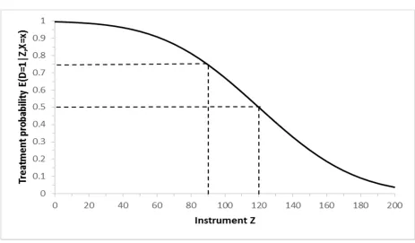
Figure 1, which is based on hypothetical data, helps to illustrate the group of compliers. Assuming a subsample with covariates fixed at , the figure depicts a continuous instrument on the horizontal axis varying between 0 and 200. The vertical axis measures the treatment probability, and the solid line displays , the treatment probability as a function of . For example, could be distance to college and college attendance. A reduction of the instrument from to raises the probability of treatment from .5 to .75. This shifts individuals with U into treatment, which are individuals who are between the 50th and 75th percentile of the distribution of . The associated LATE would thus be the treatment effect for this subgroup.
In practice, the possibility of computing all pairwise LATEs with a continuous instrument is obviously limited, as the number of observations in a given sample for every and pair is likely to be small. A useful way of exploiting a continuous instrument is therefore to partition it
14 Conversely, if a move from to shifts compliers out of treatment (
), then the associated LATE is . The only difference is that compliers are
17
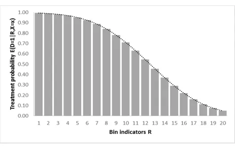
into discrete groups.15 Consider partitioning the range of in Figure 1 into equally sized bins identified by a bin identifier or grouping variable , which is a function of and assumes the integer values of 1 to 20 to indicate in which bin a given value of is situated. This is illustrated in Figure 2, where the horizontal axis is partitioned into 20 bins, and the bin height indicates the average treatment probability in each bin, . From any pair of two points and , and with corresponding data on the average outcome by bin,
conditional on , a Wald estimator of the form can be
constructed, each of which identifies LATE , a covariate-specific LATE for compliers with a move of the discretized instrument from r to r’.
2.3.2 Aggregating Pairwise (covariate-specific) LATEs into one Effect
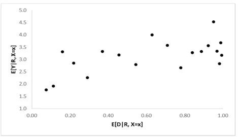
An efficient way of obtaining an overall IV estimate that aggregates the covariate-specific Wald estimates LATE across - pairs and across into one overall effect is provided by 2SLS, using group indicator dummies for the values of as instruments, fully saturating the first and second stage in the covariates, and interacting the instruments in the first stage with the covariates. As discussed in section 2.2.2 above, this provides a variance-weighted average of covariate-specific LATEs. To further see how 2SLS using group indicator dummies aggregates the pairwise LATEs across - pairs it is useful to abstract from covariates by assuming again a subsample with covariates fixed at . Figure 3 based on simulated data, which plots against helps to illustrate how the various Wald estimators are aggregated. The 2SLS estimator can be thought of as fitting a straight line through the points in Figure 3 using generalized least squares (GLS) estimation because grouped data have a known heteroscedasticity structure (Angrist, 1991). The resulting weights that each covariate-specific LATE receives are positive and sum to one. The weights are
15 It should be noted that simply using as a continuous instrument in a linear IV estimator requires
18
positively related to the strength of the first stage
and to group size (i.e., number of observation in each bin).16
Whereas it is fairly straightforward to describe for whom LATE with a single binary instrument is representative (the group of compliers with that instrument), this is no longer the case with a continuous instrument—since the overall IV effect is now representative for compliers with changes between all values of the instrument, with different weights attached to groups of compliers at different pairs of values. An aggregate IV estimate may also hide interesting information, such as which pairs of values of the instrument shift a particularly large group of individuals, or a group of individuals with particularly large treatment effects, into treatment.
2.4 Control Function Approach: The Correlated Random Coefficients Model
An alternative to conventional linear IV estimation is to use the instrument to construct a control function, and to include this into the regression alongside the endogenous variable (see Wooldridge (2015) for an overview of control function methods). A well-known model for which a control function estimator has been proposed is the correlated random coefficients model (Card, 2001; Heckman and Vytlacil, 1998; Heckman and Robb, 1985). As we explain below, the control function estimator for this model allows estimation of the ATE and yields some insight into the pattern of selection in the unobservables, albeit under stronger assumption than IV estimation. Consider the outcome equation (6) above in which we assume linearity in the regressors, and , and for a more compact notation rewrite the equation as:
(16)
16
A slope estimated by ordinary least squares is equal to a weighted average of all possible combinations of pairwise slopes between any two points, with a larger weight on slopes between points that are further apart on the
horizontal axis. This is because . In Figure 3, the
distance between two points on the horizontal axis is exactly equal to the first stage
19
with , , , , and where X denotes the
covariates centered around their sample means. This is a random coefficient model, in which the coefficient varies across individuals. Decomposing into its mean
and the deviation from the mean , equation (16) can be transformed into a constant coefficient model
(17) Here, the coefficient on is defined as the ATE. Because the covariates interacted with are centered around their mean, captures the ATE at means of , which in this linear specification is also equal to the unconditional ATE. Deviations from the ATE enter the error term . If there is selection based on gains, then and are positively
correlated, resulting in , and hence (17) is referred to as the correlated random coefficients model. Any instrument that affects will in this case also be correlated with the augmented error term . IV estimation of (17) will therefore yield a biased
estimate of (the ATE). This is not surprising because, as explained above, when treatment effects are heterogeneous IV estimation does not in general identify the ATE.
In addition to the standard assumptions of independence and existence of a first stage, assume that can be explained by the reduced-form equation
with (18)
and that both of the unobservables in that cause selection bias in (17) are linearly related to the reduced-form error :
(19) (20)
20
embodies the (rather strong) assumption that the unobserved part of the treatment effect depends linearly on the unobservables that affect the treatment.
As shown in Card (2001), under these assumptions, (17) can be estimated by OLS including and as two additional regressors (control functions), where is obtained as the predicted residual from (18) estimated by OLS.17 The estimate of is consistent for the ATE, and the sign of the coefficient on the control function is informative on the selection pattern (a positive sign implying selection based on gains). This control function approach, which can be implemented with either a binary or a continuous IV, thus yields parameters that are usually not identified by conventional IV. However, it relies on stronger assumptions than those needed for IV estimation, which does not require assumptions (18)-(20). Moreover, while it estimates ATE, it does not recover other treatment parameters, such as the ATT, ATU, or PRTE. Next, we introduce the concept of Marginal Treatment Effects (MTE) as a more informative way of exploiting a continuous instrument, which uncovers treatment effect heterogeneity more widely than the control function estimator and allows the identification of a variety of treatment parameters under potentially weaker assumptions.
3 Definition of Marginal Treatment Effects (MTE) and Relation to LATE
3.1 Definition
While LATE aggregates treatment effects over a certain range of the U distribution—see equation (15)—MTE is defined as the treatment effect at a particular value of U :
MTE U U (21)
It is thus the treatment effect for an individual with observed characteristics who are at the -th quantile of the distribution, implying these individuals are indifferent to receiving treatment when having a propensity score equal to .
17 Because of the two-step approach, standard errors need to be adjusted or bootstrapped (Wooldridge, 2015).
21
To better understand what MTEs are, abstract from covariates by assuming that we exploit a subsample with covariates fixed at . The MTE for U is the limit of LATE in equation (15) above for . The MTE at U is thus, roughly, the LATE identified from a small departure of the propensity score from value induced by the instrument.18
In formal notation, and as shown for example in Heckman, Urzúa, and Vytlacil (2006) and Carneiro et al. (2011), the MTE is identified by the derivative of the outcome with respect to the propensity score:
MTE = E (22)
Given that the Wald estimator in (13) is also a type of derivative of the outcome with respect to the treatment probability (it divides the instrument induced change in the outcome by the instrument induced change in the treatment), it may not be surprising that the MTE is identified by the derivative of the outcome with respect to the propensity score. In the following we provide some additional intuition why the derivative of the outcome with respect
to the “observed inducement into treatment” (the propensity score) yields the treatment effect
for individuals at a given point in the distribution of the unobserved resistance to treatment ( ). At a given propensity score , individuals with are treated, while individuals with are indifferent. Increasing from by a small amount shifts previously indifferent individuals into treatment, who thus have a marginal treatment effect of MTE( ). The associated increase in equals the share of shifted individuals times their treatment effect: dY= dp* MTE( ). Dividing the change in Y by the change in p (which is, roughly speaking, what a derivative does) thus gives the MTE: dY/dp= MTE( ). Therefore, the derivative of the outcome with respect to the propensity score yields the MTE at
.
18 The effect of a marginal change of the instrument as an interesting policy parameter was first introduced as
22
Figure 3 helps to interpret MTEs in an alternative way. Whereas 2SLS based on the discretized instrument fits a straight line through the grouped values in Figure 3 (the slope of
which is the aggregate IV effect), MTE can be thought of as using very fine ‘bins’ (all
available values of the propensity score) and allowing the slope of the curve to differ across values of . The local slope in a point then gives the MTE at U .
3.2 Relation to LATE and the importance of a continuous instrument
Identifying the MTE across the full range of between 0 and 1 requires a continuous instrument (at least if one wants to identify the MTE under minimal assumptions, as we discuss in section 4.2 below). The following example illustrates this. Suppose that treatment is college attendance, and that individuals continuously differ with respect to their unobserved resistance to college enrolment, . The instrument is distance to college and assume that it varies from living directly next to a college to living very far from a college. Suppose that, as depicted in Figure 1, when living right next to a college (distance of zero), all individuals attend college, even those with the highest resistance (conditional on X). In contrast, when living far away from a college, only individuals with the lowest resistance attend college (conditional on . Gradually decreasing the distance from living maximally away until living right next to a college will then gradually shift all types into college, starting from the low- types, gradually up to the high- types. Thus, everybody is a complier at some value of the continuous instrument. The wage gains associated with increases in the propensity score that result from the gradual shift in the instrument are informative on the treatment effects of each of the shifted types, and thus the marginal wage increase at a given point (the derivative with respect to ) identifies the MTE for each type.
23
between the 50th and 95th quantile of the distribution of the unobserved resistance to treatment). The associated LATE identifies thus the average over the MTE curve between
=0.5 and =0.95.
MTE is therefore defined as a continuum of treatment effects along the full distribution of U (the individual unobserved characteristic that drives treatment decisions). This has several
advantages. Firstly, rather than identifying one aggregate parameter which can mask important heterogeneity in treatment effects, the researcher is able to identify the whole (or at least a substantial part of the) range of individual treatment effects and thus characterize the extent of effect heterogeneity. Secondly, the MTE can be aggregated into economically interesting treatment effects such as the ATE, ATT, PRTE, as we show in Section 4.3. Thirdly, by relating the treatment effects to the decision of taking up the treatment measured by the participation probability, the researcher can infer the pattern of selection into treatment in a general manner along the entire unobserved resistance distribution. Estimation of the MTE is therefore more informative than both conventional IV estimator and the control function estimator of the correlated random coefficients model discussed in Sections 2.2 to 2.4 above. In the ideal case, in which the instrument varies strongly conditional on X (see Section 4.2), it requires assumptions that are no stronger than the assumptions for conventional IV estimation.
24
contrast, indicates reverse selection on gains in unobserved characteristics, while a flat MTE indicates no selection based on unobserved gains. In general, a non-monotonic shape of the MTE curve is also possible, which would imply a changing pattern of selection across the distribution of U . We provide examples of both a falling and a rising MTE curve in Section 5.
, and being residuals, their interpretation depends on the observables that are included in the regression. Changes in the variables included in X redefine the residuals and thus potentially change the MTE curve. Note however that if contains several instruments, then using them one at a time (conditioning on the respective other ones) identifies the same MTE curve (although it could identify different stretches of the MTE curve depending on the range of variation that the different instruments cause in the propensity score).
The analysis of the selection pattern in unobserved characteristics can be complemented by checking for selection on gains (or otherwise) in observed characteristics, simply by checking whether those characteristics that lead to a high in the outcome equations lead to a high in the selection equation (or otherwise).
Next, we discuss the estimation of MTEs, starting with the fully parametric normal model, which is the framework in which MTE was first introduced by Björklund and Moffitt (1987) and which relies on strong distributional assumptions.
4 Estimation of MTE
4.1 The fully parametric normal model
The parametric normal model assumes a joint normal distribution of the error terms , and V of the outcome and selection equations, V , with variance-covariance matrix in which the variance of V is normalized to 1. Moreover, suppose that potential outcomes and the selection equation are based on linear indices, that is for
25
switching regime normal selection model or Heckman selection model (Heckman, 1976). Equations (1)-(4) can be estimated either jointly by maximum likelihood or following a two-step control function procedure. The two-two-step procedure exploits the fact that the confounding endogenous variation in the error terms of the outcome equations is given by
(23)
(24)
where and denote the p.d.f and c.d.f. of the standard normal distribution, and and are the correlation coefficients between and V and and V, respectively. Based on an estimate for from a first-stage probit estimation of the selection equation one can construct estimates of the ratios in parentheses in equations (23) and (24). With these terms added as control functions, the outcome equations (1) and (2) can be estimated by OLS. The ATE conditional on X is then given by . The coefficients on the correction terms
provide estimates for the correlations and . In the normal selection model, the MTE has a parametric representation that follows directly from the joint normal distribution:19
MTE U
Not only is joint normality of V a strong assumption, it also puts strong restrictions on the shape of the MTE curve, which is simply equal to , the inverse of the standard normal c.d.f., multiplied by a constant , ruling out non-monotonic shapes of the MTE curve. If there is no selection based on unobserved gains. If , there is positive selection based on gains, and if there is reverse selection on gains. While Björklund and Moffitt (1987) first pointed out that the “marginal gain” is a relevant parameter which can be derived from the switching regime Heckman normal selection model,
19 The joint normal distribution has the property that V v v . Given that in this
26
the subsequent literature has further clarified the definition and interpretation of the MTE and, crucially, has shown how it can be derived under much weaker assumptions (essentially under the same assumptions as conventional IV estimation). We now first describe the ideal case under which the MTE can be estimated non-parametrically under minimal assumptions (which puts high demands on the data), and then the more realistic case of semi-parametric or parametric assumptions typically followed in practice (which are usually still weaker than those of the normal selection model).
4.2 Minimal assumptions and nonparametric estimation (the ideal case)
In addition to the assumptions required for a causal interpretation of the IV estimator discussed in Section 2.2, the estimation of MTE requires in the ideal case a continuous instrument Z that has enough variation conditional on to generate a propensity score P(Z) with full common support (i.e., that has support in the full unit interval for both treated and untreated individuals) conditional on . It should be noted that the “conditional on
” means within all unique combinations of the values of the ’s—a much stronger
requirement than the mere existence of a first stage. Suppose that contains two dummy variables (say, gender and race), then should have strong variation within each of the four cells defined by all possible combinations of the values for gender and race. Obviously, the more regressors are included in and the more values each regressor assumes, the stronger is this requirement.
The conventional estimation method to identify the MTE is the method of local instrumental variables (LIV – see Heckman and Vytlacil, 1999, 2001b, 2005), which estimates the MTE as the derivative of the outcome equation with respect to the propensity score, where the outcome has been modelled as a flexible function of the propensity score, thus exploiting the representation of the MTE given in equation (22) above.20
20
27
If a continuous instrument with a large range of variation within cells of is available, then the analysis can proceed in sub-samples defined by the values of , thus conditioning perfectly and non-parametrically on , and identifying a separate MTE curve for each value of . It should be noted that this allows identifying the MTE in a model with
outcome equations of the form . This “ideal” estimation approach thus does not
rely on the linear separability assumptions embodied in equations (1) and (2). Below we provide a sketch of this estimation method:
a. Split up the sample into the cells defined by and repeat the following steps separately within each of the subsamples.
b. Within each sample, estimate the probability of being treated (the propensity score) P(Z) as a function of the excluded instrument(s) . Ideally this might be done non-parametrically. Denote the predicted propensity score by .
c. Within each sample, model the outcome non-parametrically as a flexible function of (for example by local polynomial regression). Denote the predicted outcome from this flexible function as .
d. Within each sample, obtain MTE , as the derivative of with respect to , evaluated at point . Doing this for a grid of values for from 0 to 1 allows tracing out the MTE curve for the full unit interval.21
4.3 Strengthening assumptions for estimation in less ideal cases
The approach outlined in the previous section assumes the availability of an ideal continuous instrument with sufficient variation conditional on to generate a propensity score P(Z) with full common support conditional on . This is rarely available, and
21
28
additional assumptions need to be made. A first assumption is to not condition on X fully non-parametrically, but in a parametric linear way and model potential outcomes as
and and the selection equation as
.
A second assumption restricts the shape of the MTE curve to be independent of (common across all values of ), except for the intercept of the MTE curve which is allowed to vary with . Independence of the shape of the MTE curve across X is implied by the full independence assumption X , which is stronger than the conditional independence assumption necessary for a causal interpretation of IV and the estimation of MTE in the ideal case. Full independence not only implies that X is exogenous, but also that the way in which and depend on , and therefore the shape of the MTE curve, does not depend on X.22 Alternatively, rather than invoking full independence, one can, in addition to the conditional independence assumption, assume additive separability between an observed and an unobserved component in the expected potential outcomes conditional on U (Brinch et al., 2015):
U U
Both, the full independence and the linear separability assumption, imply that the marginal treatment effect defined in equation (21) is additively separable into an observed and an unobserved component:23
MTE U
U (25)
Exploiting linearity of the outcome in X and a constant shape of the MTE across X (except for a varying intercept) leads to the following outcome equation:
22 Full independence between (X, ) and U U U
D is for example invoked in Aakvik, Heckman, and
Vytlacil 2005; Carneiro et al., 2011; and Carneiro et al., 2015.
23
29
(26) where is a nonlinear function of the propensity score. The coefficients on the interaction terms of and identify and show how observed characteristics shift the treatment effect (and thus the intercept of the MTE curve). The fact that does not depend on X reflects the assumption that the slope of the MTE curve in does not depend on . Crucially, this allows identifying across all values of , instead of within all values of , and it therefore only requires unconditional full common support of the propensity score (across all values of ), an assumption which is in many applications more realistically obtainable than full common support conditional on . From equation (22), the MTE is then given by
MTE
As before, estimation of the outcome equation requires a pre-estimated propensity score from a first stage estimation in order to estimate the second stage outcome equation given in (26). Estimation of MTE then proceeds by making varying degrees of functional form assumptions on Heckman et al. (2006) propose a semi-parametric estimation method for (26). A more parametric approach is to model as a polynomial in which nevertheless allows for considerably more flexibility than the parametric normal model described in section 4.1.
We provide a brief sketch of the semi-parametric and parametric polynomial approaches in Appendix B. The semi-parametric, parametric polynomial, and the normal model are all implemented in Stata by the user-written margte command and an accompanying Stata Journal article is available (see Brave and Walstrum, 2014). Further documentation on estimation techniques is also available in the supplementary online material of Heckman et al. (2006).24
30
4.4 Aggregating the MTE into treatment parameters
An important advantage of MTE estimation is that the MTE equation (21) can be aggregated into weighted averages over X and U to generate aggregate treatment parameters, such as ATE, TT, TUT and PRTE, or the IV effect associated with a given instrument. Heckman and Vytlacil (2005, 2007) present weights that aggregate the MTE curve along the U -dimension, conditional on X x, which then recover aggregate treatment parameters
conditional on X x. One may want to further aggregate these conditional parameters over the appropriate distribution of X in order to obtain unconditional aggregate treatment parameters. While in theory U is continuous (and the MTE weights are therefore often presented in continuous form), an applied researcher will usually calculate the MTE along a grid of values of U and will therefore in practice face a discrete distribution of U . Here we present unconditional treatment effects computed from a discrete distribution of U . We present the IV weights under the assumptions that potential outcomes are linear in (i.e., and and that the MTE is linearly separable into its observed and unobserved part, as in equation (25), where the unobserved part is normalized to a mean of zero. These assumptions are in line with the applied MTE literature and the strengthened set of assumptions discussed in section 4.3 above. We denote the sample size by N, index individual observations by i, denote the propensity score by and define as the propensity score averaged over all individuals.
An equally weighted average of the MTE over the full distribution of X and U yields the unconditional average treatment effect (ATE) defined in equation (7):
observed component of MTE at sample means
U
equally weighted average over unobserved component of MTE
(27)
31
On the other hand, the treatment effect on the treated (TT) defined in equation (8) is an average of the MTE over individuals whose U is such that at their given values of and (and thus a given propensity score, ), they choose to take the treatment. It can be represented by
observed component of MTE at means of treated
U
weighted average over unobserved component of MTE giving more weight to low UD individuals
(28)
Note that the observed characteristics are weighted such that observations with a higher propensity score (and thus higher treatment probability) get a higher weight—which corresponds to using observed means of of the treated subpopulation, as implied by equation (8). In the unobserved component, the weight of a given value of u is related to the share of observations that have a propensity score higher than u . Thus, low-u individuals (with unobserved characteristics that make them more likely to be treated) get a higher weight, and the weight depends on the distribution of the propensity score (note that while U is by construction uniformly distributed, the distribution of is an empirical question).
Replacing in the observed component by and in the unobserved
component by yields the equivalent expression for the TUT defined by equation (9).
The TUT weights the observed part of the treatment effect more strongly for individuals with a low propensity score (and thus low probability of treatment)—which corresponds to using observed means of of the untreated subpopulation, as implied by equation (9). The TUT additionally weights the unobserved part more strongly for individuals at the higher end of the U distribution who have a stronger unobserved resistance to treatment.
32
U
(29)
Both, observed and unobserved characteristics are weighted proportionately to the policy-induced change in the probability of being treated for individuals with given characteristics. Individual observed characteristics are weighted proportionately to the change in the individual propensity score ( ), and each value u of the unobserved characteristic is weighted proportionately to the change in the probability of being treated at that value,
u .
Finally, it is possible to calculate IV weights, which recover the IV effect when using a specific instrumental variable. Denoting the IV weights using J as an instrument conditional on
X and U by IV , the IV effect can be expressed as
IV
observed component of MTE at means of individuals shifted by the instrument
IV U (30)
The weights on the observed characteristics are similar to the weights discussed in section 2.2.2 above and are proportionate to the contribution of individuals with to the IV first-stage covariance – see footnote 12 above. The weights on the unobserved part depend on the effect of on at different levels of , weighted by the distribution of . More detail on the estimation of these weights is provided in Appendix C.
33
5 Two examples from the applied literature
5.1 Example of MTE applied to returns to college education
Carneiro et al. (2011) analyze the marginal returns to college attendance for the United States, based on a sample of white males from the NLSY aged 28-34 in 1991. The binary treatment, , is defined as having ever been enrolled in college by 1991. Hence, =0 for high school dropouts and high school graduates and =1 for individuals with some college, college graduates as well as postgraduates. The outcome, , is the log wage in 1991. As instrumental variables ( in our above notation) that enter the selection equation but not the outcome equation, the authors draw on four instruments, some binary and some continuous, that have been used in previous studies on the returns to college attendance. These are on the one hand cost-shifters (i.e., the presence of a four-year college and average tuition fees in public four year colleges in the county of residence during adolescents), and on the other hand variables capturing local labor market opportunities at the time the education decision is taken (i.e., the local average earnings and the local unemployment rate).25 The instrumental variables, which each identify a different part of the MTE curve, are included simultaneously in order to get larger support in the propensity score. Carneiro et al. (2011) further control for individual’s socio-economic background and measures of permanent local labor market characteristics ( in our notation).
In their main specification, the authors invoke the assumption of full independence X Z , implying that the shape of the MTE curve does not vary with X and the
MTE can thus be identified over the unconditional (marginal) support of the propensity score (see Section 4.3).26 They then estimate the MTE using the semi-parametric estimation method outlined in Appendix B.1, which allows for a completely flexible shape of the MTE curve.
25
The number of IVs is further expanded by interacting these variables with an ability measure (Armed Forces Qualification Test - AFQT), mother’s years of schooling, and number of siblings.
26
34
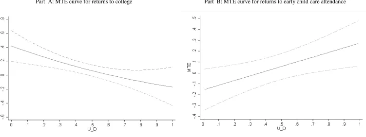
Part A of Figure 4 depicts the MTE curve U – see equation (25) above – evaluating at mean values in the sample. The figure reveals substantial heterogeneity in the returns to college: Whereas individuals with “low resistance” to college (i.e., very low U enjoy returns of 40%, individuals with “high resistance” to college (i.e., very high U lose from college by 20%. This large range of heterogeneity in the treatment effect due to unobserved characteristics would not be visible if looking only at aggregate treatment effects such as ATE. Since these returns refer to individuals with average X, heterogeneity in returns will be even greater when variation in X is taken into account. The downward sloping shape of the MTE curve highlights high gains for individuals likely to enroll in college (low U and lower gains, or even losses, for individuals less likely to enrol in college (high U . Thus, individuals positively select into college based on gains, and individuals seem to possess information about their idiosyncratic returns and are able to make informed choices about college attendance.
35
5.2 Example of MTE applied to returns to preschool education
Cornelissen et al. (2016) analyzes heterogeneous treatment effects of a universal child care (preschool) program aimed at 3- to 6-year-olds on children’s school readiness. They draw on
administrative data on children’s outcomes from school readiness examinations for the full
population of school entry aged children in one large region in Germany for the years
1994-2002. The authors exploit a reform during the 1990s that entitled every child in Germany to a heavily subsidized half-day child care placement from the third birthday to school entry. This reform was enacted in response to a severe shortage of child care slots which rationed in
particular children who wanted to enroll at the earliest possible age (at age 3).27 As a result, the reform greatly increased the share of children enrolling at the earliest possible age and thus
attending child care for at least 3 years from 41% to 67% on average over the program rollout
period. Correspondingly, the treatment, , is defined as attending child care for at least 3 years
and referred to as “early attendance”. Their main outcome variable, , is a measure of overall
school readiness (which determines whether the child is held back from school entry for
another year). As an instrument (denoted by in our notation above) the authors use the
supply of available child care slots at the municipality-year level measured by the child care
coverage rate, a continuous variable.28 The control variables ( in our above notation) include
municipality and examination cohort dummies in addition to individual characteristics such as ethnic minority status, and average socio-demographic characteristics and child-care quality indicators at municipality-year level.
Similar to the previous example, the authors also exploit the marginal support of the
propensity score (rather than the support conditional on in the ideal case), but based on the linear separability assumption described in Section 4.3 above, rather than the full independence
assumption invoked in Carneiro et al. (2011). Their preferred estimation method is the
27
Children who wanted to enter at an older age (who may already have waited on the waiting list for one year) were generally given priority.
28 Linear and squared terms of the instrument are included, and in the main specification both of these terms
36
parametric polynomial approach with a second order polynomial in the propensity score (see Appendix B.2). This model restricts the MTE curve to a straight line and thus appears equally restrictive as the normal section model (in that it rules out a non-monotonic shape). To rule out
concerns that this restrictive choice drives their results, the authors show that their main pattern of results is robust to estimating more flexible MTE curves by using higher-order polynomials
or implementing the semi-parametric estimation method.
Part B of Figure 4 depicts the resulting linear MTE curve, evaluated at mean values of X in the sample. In contrast to the previous example, the MTE curve now exhibits an upward
sloping shape, indicating a pattern of reverse selection on gains. Whereas children with low
resistance to prolonged child care attendance (low U do not gain, improvements in school readiness are substantial for children with a high resistance to prolonged child care attendance
(high U In consequence, the TUT—which indicates that early child care attendance would
boost school readiness of children currently not enrolled in child care by 17.3 percentage points—exceeds the ATE and TT, neither of which is statistically significant (see column (2)
of Table 1).29
As in Carneiro et al. (2011), the linear IV estimate turns out to be similar in magnitude to
ATE and masks important heterogeneity in returns. Moreover, the linear IV effect estimated by 2SLS is very similar to the effect obtained when applying the IV weights to the MTE curve, which can be considered a specification check for the functional form of the MTE curve.30
The authors confirm a pattern of reverse selection on gains also based on observed characteristics. For example, minority children are 12 percentage points less likely to attend
preschool, but their treatment effect is about 12 percentage points higher than for majority
29 Kline and Walters (2015) uncover a pattern of reverse selection on gains for Head Start attendance when
the nontreated state is home care. Aakvik et al. (2005) find reverse selection on gains in the context of a Vocational Rehabilitation training program.
30