Simultaneous determination of time-dependent coefficients and heat source

This is a repository copy of Simultaneous determination of time-dependent coefficients and heat source.

White Rose Research Online URL for this paper: http://eprints.whiterose.ac.uk/104369/

Version: Accepted Version

Article:

Hussein, MS and Lesnic, D (2016) Simultaneous determination of time-dependent coefficients and heat source. International Journal for Computational Methods in Engineering Science and Mechanics, 17 (5-6). pp. 401-411. ISSN 1550-2287 https://doi.org/10.1080/15502287.2016.1231241

(c) 2016, Taylor & Francis Group, LLC. This is an Accepted Manuscript of an article published by Taylor & Francis in the International Journal for Computational Methods in Engineering Science and Mechanics on 14th October 2016, available online:

https://doi.org/10.1080/15502287.2016.1231241

[email protected] https://eprints.whiterose.ac.uk/ Reuse

Unless indicated otherwise, fulltext items are protected by copyright with all rights reserved. The copyright exception in section 29 of the Copyright, Designs and Patents Act 1988 allows the making of a single copy solely for the purpose of non-commercial research or private study within the limits of fair dealing. The publisher or other rights-holder may allow further reproduction and re-use of this version - refer to the White Rose Research Online record for this item. Where records identify the publisher as the copyright holder, users can verify any specific terms of use on the publisher’s website.

Takedown

If you consider content in White Rose Research Online to be in breach of UK law, please notify us by

Simultaneous determination of time-dependent

coefficients and heat source

M.S. Hussein1,2 _{and D. Lesnic}1

1_{Department of Applied Mathematics, University of Leeds, Leeds LS2 9JT, UK}

2_{Department of Mathematics, College of Science, University of Baghdad, Baghdad, Iraq}

E-mails: [email protected] (M.S. Hussein), [email protected] (D. Lesnic).

Abstract

This paper presents a numerical solution to the inverse problems of simultaneous deter-mination of the time-dependent coefficients and the source term in the parabolic heat equation subject to overspecified conditions of integral type. The ill-posed problems are numerically discretised using the finite-difference method and the resulting system of nonlinear equations is solved numerically using the MATLAB toolbox routine lsqnonlin

applied to minimizing the nonlinear Tikhonov regularization functional subject to simple physical bounds on the variables. Numerical examples are presented to illustrate the ac-curacy and stability of the solution.

Keywords: Inverse problem; Coefficient identification; Heat equation; Finite-difference method; Tikhonov regularization; Nonlinear minimization.

1

Introduction

Determination of a single unknown time-dependent property such as the capacity, conduc-tivity or diffusivity from additional local or non-local measurements of the main dependent variable at the boundary or inside the space domain represents a classical example of a coefficient identification problem, as described for example in Chapter 13 of the excellent book of Cannon [4] on the one-dimensional heat equation. For more recent studies on the same inverse problems, see e.g. [9, 13] and the references therein.

The inverse formulation can be further extended to allow for an unknown free boundary to be determined as well, see e.g. [12]. Moreover, multiple time-dependent coefficient identifications have also been considered theoretically in the past, see e.g. [3, 11], and recently been solved numerically by the authors, [8]. In these studies, the unknowns were mainly coefficients multiplying the temperature and its partial derivatives, but more recent theoretical studies, [14, 15], allow for one of the time-dependent unknown to be in the free term heat source as well. And it is the purpose of this paper to numerically solve a couple of such related multiple coefficient identification problems.

2

Mathematical formulation

In this paper, we study a couple of coefficient identification problems related to the second-order parabolic partial differential equation

∂u

∂t(x, t) =a(x, t)

∂2_u

∂x2(x, t)−b(x, t)

∂u

∂x(x, t)−d(x, t)u(x, t) +f(t)g(x, t), (x, t)∈QT.

(1)

whereQT = [−ℓ, ℓ]×[0, T], with ℓ >0 andT > 0, represents the solution domain,a(x, t) is a given positive function involving physical quantities of the medium (−ℓ, ℓ) such as conductivity, capacity, storage, diffusivity,u(x, t) is the unknown dependent variable, e.g. the temperature in heat conduction, the pressure in porous media or the piezometric head in groundwater flow, f(t)g(x, t) with f(t) unknown and g(x, t) given function rep-resents a source (heat or hydraulic), and either one of the coefficientsb (representing an advection/convection coefficient) or d (representing a reaction or perfusion coefficient in bio-heat conduction) are unknown (though we shall further assume that, when unknown, the corresponding quantity b or d depends on time only). To be more explicit, let us particularize equation (1) to the following two cases, namely,

∂u

∂t(x, t) = a(x, t)

∂2_u

∂x2(x, t)−b(t)

∂u

∂x(x, t)−d(x, t)u(x, t) +f(t)g(x, t), (x, t)∈QT (2)

with unknown triplet (u(x, t), f(t), b(t)) and

∂u

∂t(x, t) =a(x, t)

∂2_u

∂x2(x, t)−b(x, t)

∂u

∂x(x, t)−d(t)u(x, t) +f(t)g(x, t), (x, t)∈QT. (3)

with unknown triplet (u(x, t), f(t), d(t)).

We emphasize that such particularizations are often necessary when seeking to es-tablish the uniqueness of the solution. Together with (2) or (3) we impose the initial condition

u(x,0) =ϕ(x), x∈[−ℓ, ℓ], (4)

and the homogenous Dirichlet boundary conditions

u(±ℓ, t) = 0, t∈[0, T]. (5)

As over-determination conditions we consider, [14],

∫ ℓ

−ℓ

ω(x)u(x, t)dx=φ(t), t∈[0, T], (6)

∫ ℓ

−ℓ

ω(x)ux(x, t)dx=ψ(t), t∈[0, T], (7)

of an object (or a process) at individual points and instead only the mean value of the state over the entire object can be specified, [1]. Remark also that if ω is differentiable then integration by parts in (7) and using (5) imply

∫ ℓ

−ℓ

ω′

(x)u(x, t)dx=−ψ(t), t∈[0, T], (8)

so (7) may be thought to have the same physical meaning as (6) previously described. About the input data we assume that they satisfy the following conditions:

(A) 0< a0 ≤a(x, t)≤a1, |ax(x, t)| ≤Ka∗, |axx(x, t)| ≤Ka∗∗, (x, t)∈QT.

(B) |g(x, t)| ≤Kg, (x, t)∈QT.

(C) ω ∈W3

∞([−ℓ, ℓ]),ω(±ℓ) =ω ′

(±ℓ) = 0, |ω′′

(x)| ≤K∗∗

ω ,x∈[−ℓ, ℓ],

∫ℓ

−ℓω(x)ϕ(x)dx=

φ(0), ∫ℓ

−ℓω(x)ϕ ′

(x)dx=ψ(0).

(D) ϕ ∈

◦

W1

2([−ℓ, ℓ]), |ϕ(x)| ≤M0,x∈[−ℓ, ℓ].

(E) φ(t), ψ(t)∈W1

∞([0, T]).

For the notation of the spaces of functions involved, see [16]. Then we have the following theorems of uniqueness of the solution for the inverse problems considered.

Theorem 1 (see [14]). Assume conditions (A)–(E) on the input data hold. Assume also

that0< ψ0 ≤ |ψ(t)|, t∈[0, T], |d(x, t)| ≤d1, (x, t)∈QT, and that

∫ ℓ

−ℓ

ω′

(x)g(x, t)dx

≥G0 >0, t∈[0, T]. (9)

In addition, let the inequality

2ℓ|G1(t)|Kω∗∗(M0+KgT R0)ed1T ≤ 1

2G0ψ0, t∈[0, T], (10)

hold for some R0 >0, where

G1(t) =

∫ ℓ

−ℓ

ω(x)g(x, t)dx, t∈[0, T]. (11)

Then there exists at most one solution

(u(x, t), f(t), b(t))∈(

W₂1,2(QT)∩C0,α(QT)

)

×L∞([0, T])×L∞([0, T]), (12) for someα ∈(0,1), of the inverse problem (2), (4)–(7) such that

∥f∥L∞([0,T]) ≤R0. (13)

In particular, if it happens that G1(t) ≡ 0 on [0, T] then (10) holds for any R0 >0 and

thus the uniqueness of solution holds without the restriction (13).

Theorem 2 (see [15]). Assume conditions (A)–(E) on the input data hold. Assume also that|b(x, t)| ≤Kb, |bx(x, t)| ≤Kb∗, (x, t)∈QT, and that

∆1(t) : =ψ(t)

∫ ℓ

−ℓ

ω(x)g(x, t)dx+φ(t)

∫ ℓ

−ℓ

ω′

(x)g(x, t)dx≥δ1 >0, t∈[0, T]. (14)

Then there exists at most one solution

(u(x, t), f(t), d(t))∈(

W₂1,2(QT)∩C0,α(QT)

)

3

Numerical Solution of the Direct Problem

In this section, we consider the direct (forward) initial value problem given by equations (1), (4) and (5) when the coefficientsb(x, t),d(x, t) and f(t) are given and the dependent variable u(x, t) is the solution to be determined. We use the finite-difference method (FDM) with Crank-Nicolson scheme, [18], which is unconditionally stable and second order accurate in space and time.

The discrete form of the direct problem is as follows. Taking the positive integer numbersM andN, the solution domainQT = [−ℓ, ℓ]×[0, T] is divided by aM×N mesh with spatial step size ∆x = 2ℓ/M in x-direction and the time step size ∆t =T /N. The solution at the node (i, j) is denoted by ui,j :=u(xi, tj), wherexi =−ℓ+i∆x, tj =j∆t,

ai,j := a(xi, tj), bi,j := b(xi, tj), fj := f(tj) =, di,j := d(xi, tj) and gi,j := g(xi, tj) for

i= 0, M and j = 0, N.

Considering the general form of partial differential equation

ut=G(x, t, u, ux, uxx), (16)

equation (16) can be approximated as

ui,j+1−ui,j

∆t =

1

2(Gi,j+Gi,j+1), i= 1, M , j = 0,(N −1), (17)

ui,0 =ϕ(xi), i= 0, M , (18)

u0,j = 0, uM,j = 0, j = 0, N , (19)

where

Gi,j =G

(

xi, tj,

ui+1,j−ui−1,j 2(∆x) ,

ui+1,j−2ui,j+ui−1,j (∆x)2

)

, i= 1,(M −1), j = 0, N . (20)

For our problem, equation (1) can be discretised in the form of (17) as

−Ai,j+1ui−1,j+1+ (1 +Bi,j+1)ui,j+1−Ci,j+1ui+1,j+1 =

Ai,jui−1,j+ (1−Bi,j)ui,j +Ci,jui+1,j+ ∆t

2 (fjgi,j +fj+1gi,j+1), (21)

fori= 1,(M−1), j = 0,(N −1), where

Ai,j =

(∆t)ai,j 2(∆x)2 +

bi,j(∆t)

4(∆x) , Bi,j =

(∆t)ai,j (∆x)2 +

∆t

2 di,j, Ci,j =

(∆t)ai,j 2(∆x)2 −

bi,j(∆t)

4(∆x) .

At each time step tj+1, for j = 0,(N−1), using the homogenous Dirichlet boundary conditions (19), the above difference equation can be reformulated as a (M−1)×(M−1) system of linear equations of the form,

Duj+1 = Euj+b, (22)

where

D=       

1 +B1,j+1 −C1,j+1 0 · · · 0 0 0

−A2,j+1 1 +B2,j+1 −C2,j+1 · · · 0 0 0

... ... ... . .. ... ... ...

0 0 0 · · · −AM−2,j+1 1 +BM−2,j+1 −CM−2,j+1

0 0 0 · · · 0 −AM−1,j+1 1 +BM−1,j+1

       , E =       

1−B1,j C1,j 0 · · · 0 0 0

A2,j 1−B2,j C2,j · · · 0 0 0

... ... ... ... ... ... ...

0 0 0 · · · AM−2,j 1−BM−2,j CM−2,j

0 0 0 · · · 0 AM−1,j 1−BM−1,j

       , and b=        ∆t

2 (fjg1,j +fj+1g1,j+1) ∆t

2 (fjg2,j +fj+1g2,j+1) ...

∆t

2 (fjgM−2,j +fj+1gM−2,j+1)

∆t

2 (fjgM−1,j +fj+1gM−1,j+1)

       .

The numerical solutions forφ(t) and ψ(t) are calculated using the trapezoidal rule for integrals in (6) and (7), namely,

φ(tj) =

∫ ℓ

−ℓ

ω(x)u(x, tj)dx= ∆x

(_M−1

∑

i=1

ui,jωi

)

, j = 0, N , (23)

ψ(tj) =

∫ ℓ

−ℓ

ω(x)ux(x, tj)dx=

∆x

2

(

ux0,jω0+uxM,jωM + 2

M−1

∑

i=1

uxi,jωi

)

, j = 0, N ,

(24)

whereωi :=ω(xi) for i= 0, M, and

ux0,j =

4u1,j −u2,j−3u0,j

2(∆x) , uxM,j =−

4uM−1,j−uM−2,j−3uM,j

2(∆x) ,

uxi,j =

ui+1,j−ui−1,j

2(∆x) , i= 1,(M −1), j = 0, N .

4

Numerical Solutions of the Inverse Problems

In this section, we aim to obtain accurate and stable simultaneous identifications for the temperature u(x, t), source f(t) and the coefficients b(t) or d(t) for the inverse prob-lems (2), (4)–(7) or (3)–(7), respectively. In the former case we minimize the nonlinear Tikhonov functional

F1(b, f) : =

∫ ℓ

−ℓ

ω(x)u(x, t)dx−φ(t)

2 + ∫ ℓ −ℓ

ω(x)ux(x, t)dx−ψ(t)

2

+β1

b(t)

2 +β2

f(t)

2

whilst in the latter case we minimize

F2(d, f) : =

∫ ℓ

−ℓ

ω(x)u(x, t)dx−φ(t)

2 + ∫ ℓ −ℓ

ω(x)ux(x, t)dx−ψ(t)

2

+β3

d(t)

2 +β2

f(t)

2

, (26)

where βi ≥0, i = 1,2,3, are regularization parameters which are introduced in order to stabilise the numerical solution and the norm is theL2_{[0, T] norm. The discretizations of} (25) and (26) are

F1(b, f) :=

N

∑

j=1

[∫ ℓ −ℓ

ω(x)u(x, tj)dx−φ(tj)

]2

+ N

∑

j=1

[∫ ℓ −ℓ

ω(x)ux(x, tj)dx−ψ(tj)

]2

+β1 N

∑

j=1

b2j +β2

N

∑

j=1

fj2, (27)

F2(d, f) :=

N

∑

j=1

[∫ ℓ −ℓ

ω(x)u(x, tj)dx−φ(tj)

]2

+ N

∑

j=1

[∫ ℓ −ℓ

ω(x)ux(x, tj)dx−ψ(tj)

]2

+β3 N

∑

j=1

d2_j +β2

N

∑

j=1

f_j2. (28)

respectively.

The unregularized case, i.e., βi = 0 for i = 1,2,3, yields the ordinary nonlinear least-squares method which is usually producing unstable solutions when noisy data are inverted.

The noisy data is numerically simulated as

φϵ1(tj) =φ(tj) +ϵ1j, ψϵ2(tj) =ψ(tj) +ϵ2j, j = 1, N , (29)

where ϵ1j and ϵ2j are random variables generated from a Gaussian normal distribution with mean zero and standard deviationσ1 and σ2, respectively, given by

σ1 =p× max

t∈[0,T]|φ(t)|, σ2 = p×tmax∈[0,T]|ψ(t)|, (30)

where p represents the percentage of noise. We use the MATLAB function normrnd to generate the random variablesϵ1 = (ϵ1j)_j=1,N and ϵ2 = (ϵ2j)_j=1,N as follows:

ϵ1 =normrnd(0, σ1, N), ϵ2 = normrnd(0, σ2, N). (31)

In the case of noisy data (6) and (7), we replace φ(tj) and ψ(tj) by φϵ1(tj) and ψϵ2(tj), respectively, in (27) and (28).

The minimization ofF1orF2subject to simple bounds on the variables is accomplished using the MATLAB optimization toolbox routinelsqnonlin, which does not require sup-plying (by the user) the gradient of the objective function, [17]. This routine attempts to find a minimum of a sum of squares, starting from an initial guess, subject to constraints and this generally is referred to as a constrained nonlinear optimization.

• Maximum number of iterations = 10×(number of variables).

• Maximum number of objective function evaluations = 105_{×(number of variables).}

• Solution tolerance = 10−10_.

• Object function tolerance = 10−10_.

5

Numerical Results and Discussion

In this section, we present numerical results for the recovery of the unknownsf(t),b(t) or

d(t), in the case of exact and noisy data (29). To measure the accuracy of the numerical solution we employ the root mean square error (rmse) defined by:

rmse(f) =

v u u t

1

N

N

∑

j=1

(fnumerical(tj)−fexact(tj))2, (32)

and similar expressions exist forb(t) and d(t).

Remark 1.

During the computation we need the values of f(0) and b(0) or d(0). One can easily derive these values from the governing equations (2) or (3) with the help of the initial and boundary conditions (4) and (5), as follows.

Apply (2) or (3) at x=±ℓ to obtain

ut(±ℓ, t) =a(±ℓ, t)uxx(±ℓ, t)−b(t)ux(±ℓ, t)−d(±ℓ, t)u(±ℓ, t) +f(t)g(±ℓ, t), (33)

or

ut(±ℓ, t) =a(±ℓ, t)uxx(±ℓ, t)−b(±ℓ, t)ux(±ℓ, t)−d(t)u(±ℓ, t) +f(t)g(±ℓ, t), (34)

respectively. Then apply (33) and (34) att= 0, and use the compatibility conditions for the initial data (4) and the boundary conditions (5) to result in

0 =a(±ℓ,0)ϕ′′

(±ℓ)−b(0)ϕ′

(±ℓ) +f(0)g(±ℓ,0), (35)

or

0 = a(±ℓ,0)ϕ′′

(±ℓ)−b(±ℓ,0)ϕ′

(±ℓ) +f(0)g(±ℓ,0), (36)

respectively. Solving the (2×2) linear system of equations (35) for b(0) and f(0) we obtain

b(0) = −g(−ℓ,0)a(ℓ,0)ϕ

′′

(ℓ) +g(ℓ,0)a(−ℓ,0)ϕ′′

(−ℓ)

−ϕ′_{(−ℓ)g(ℓ,0) +ϕ}′_{(ℓ)g(−ℓ,0)} , (37)

f(0) = ϕ

′

(−ℓ)a(ℓ,0)ϕ′′

(ℓ) +ϕ′

(ℓ)a(−ℓ,0)ϕ′′

(−ℓ)

−ϕ′_{(−ℓ)g(ℓ,0) +ϕ}′_{(ℓ)g(−ℓ,0)} , (38)

provided that the denominator −ϕ′

(−ℓ)g(ℓ,0) +ϕ′

(ℓ)g(−ℓ,0) ̸= 0. Also, from equation (36) an expression forf(0) can be obtained as

f(0) = −a(±ℓ,0)ϕ

′′

(±ℓ) +b(±ℓ,0)ϕ′

(±ℓ)

provided that the denominator g(±ℓ,0) ̸= 0. For d(0) we use a different method which uses the overdermination conditions (6) or (7), as follows. Multiplying equation (3) by

ω(x) and integrating with respect to x, using (6), we obtain

φ′

(t) =

∫ ℓ

−ℓ

ω(x)(a(x, t)uxx(x, t)−b(x, t)ux(x, t))dx−d(t)φ(t)

+f(t)

∫ ℓ

−ℓ

ω(x)g(x, t)dx. (40)

Settingt= 0 in (40) we obtain

d(0) = −φ

′

(0) +∫ℓ

−ℓω(x) (a(x,0)ϕ

′′

(x)−b(x,0)ϕ′

(x))dx+f(0)∫ℓ

−ℓω(x)g(x,0)dx

φ(0) , (41)

provided thatφ(0)̸= 0, wheref(0) is computed by expression (39). Alternatively, differ-entiating equation (3) with respect tox and multiplying it by ω(x) and then integrating it with respect to x, and using (7), we obtain

ψ′

(t) =

∫ ℓ

−ℓ

ω(x)[(a(x, t)uxx(x, t))x−(b(x, t)ux(x, t))x]dx−d(t)ψ(t)

+f(t)

∫ ℓ

−ℓ

ω(x)gx(x, t)dx. (42)

Settingt= 0 in (42) we obtain

d(0) = −ψ

′

(0) +∫ℓ

−ℓω(x) (a(x,0)ϕ

′′

(x)−b(x,0)ϕ′

(x))′

dx+f(0)∫ℓ

−ℓω(x)gx(x,0)dx

ψ(0) ,

(43)

provided that ψ(0)̸= 0, where f(0) is computed by expression (39).

5.1

Example 1

Consider first the inverse problem (2), (4)–(7), with unknown coefficients f(t) and b(t), and the following input data:

a(x, t) = 1, d(x, t) = 0, g(x, t) =−x3, (x, t)∈QT, (44)

ϕ(x) = x(ℓ2−x2), ω(x) = (x2−ℓ2)2, x∈[−ℓ, ℓ], (45)

φ(t) =

∫ ℓ

−ℓ

ω(x)u(x, t)dx= 0, t∈[0, T], (46)

ψ(t) =

∫ ℓ

−ℓ

ω(x)ux(x, t)dx=

64ℓ7_e−6t

105 , t∈[0, T]. (47)

One can easily observe that the conditions of Theorem 1 are satisfied by the above input data (in particular note that G1(t) =

∫ℓ

−ℓω(x)g(x, t)dx = − ∫ℓ

−ℓx

hence the inverse problem has at most one solution in the class of functions (12). In fact, it can easily be checked by direct substitution that the analytical solution is given by

b(t) = 0, f(t) =−6e

−6t ℓ2

ℓ2 , t∈[0, T], (48)

u(x, t) = e−ℓ62tx(ℓ2−x2), (x, t)∈Q

T. (49)

We take for simplicity, ℓ = T = 1 and employ the FDM described in Section 3 with

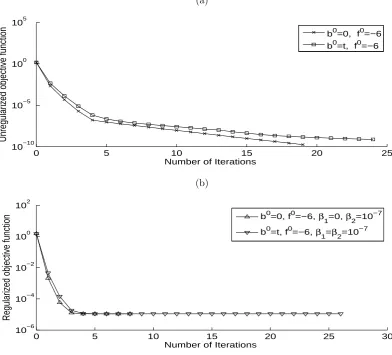
M=N=40 at each iteration of minimization procedure described in Section 4. Remark that from (37) and (38) we obtain b(0) = 0 and f(0) = −6 and therefore, appropriate candidates for the initial guesses of b and f are b0 _{= 0 and f}0 _{=−6. However, because} the exact solution for b(t) is actually the trivial zero function we also investigate another initial guess forb given by b0_{(t) = t.}

(a)

0 5 10 15 20 25

10−10 10−5 100 105

Number of Iterations

Unregularized objective function

b0=0, f0=−6 b0=t, f0=−6

(b)

0 5 10 15 20 25 30

10−6 10−4 10−2 100 102

Number of Iterations

Regularized objective function

b0=0, f0=−6, β

1=0, β2=10 −7

b0=t, f0=−6, β

1=β2=10 −7

Figure 1: The objective function (27), (a) without and (b) with regularization, and various initial guesses, for Example 1 with exact data.

(a)

0 0.1 0.2 0.3 0.4 0.5 0.6 0.7 0.8 0.9 1 −0.2

0 0.2 0.4 0.6 0.8

t

b(t)

(b)

0 0.1 0.2 0.3 0.4 0.5 0.6 0.7 0.8 0.9 1 −6

−4 −2 0 2

t

f(t)

(a)

0 0.1 0.2 0.3 0.4 0.5 0.6 0.7 0.8 0.9 1 −1

−0.5 0 0.5 1 1.5

2x 10

−3

t

b(t)

(b)

0 0.1 0.2 0.3 0.4 0.5 0.6 0.7 0.8 0.9 1 −6

−5 −4 −3 −2 −1 0

t

f(t)

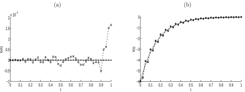
Figure 3: The exact (—) and numerical solutions with regularization and various initial guesses b0 = 0, β1 = 0, β2 = 10−7 (-× -) andb0 =t,β1 =β2 = 10−7 (- -) for: (a) b(t) and (b) f(t),

for Example 1 with exact data.

In the remaining of this subsection, for brevity, we only illustrate the results obtained with the initial guess b0 _{=t and f}0 _=−6.

Table 1: Number of iterations, number of function evaluations, value of the objective function (27) at final iteration, thermse values and the computational time with and without regular-ization and various initial guesses for Example 1 with exact data.

β1 =β2 = 0 b0 = 0, f0 =−6 b0 =t, f0 =−6

No. of iterations 19 24

No. of function evaluations 1660 2075

Value of objective function (27) at final iteration

1.7E-10 7.4E-10

rmse(b) 6.1E-6 0.1557

rmse(f) 0.4379 0.4536

Computational time 20 mins 24 mins

β2 = 10−7 b0 = 0, f0 =−6, β1 = 0 b0 =t, f0 =−6,β1 = 10−7

No. of iterations 8 9

No. of function evaluations 747 830

Value of objective function (27) at final iteration

1.0E-5 1.0E-5

rmse(b) 3.5E-6 4.0E-4

rmse(f) 0.1514 0.1516

Computational time 9 mins 10 mins

for both coefficients b(t) and f(t) (compare with the results for exact data in Figure 2). This is expected since the problem under investigation is ill-posed. Consequently, regularization should be applied to restore the stability of the solution in the components

b(t) and f(t).

100 101 102 103

10−15 10−10 10−5 100

Number of Iterations

Unregularized objective function

Figure 4: The objective function (27) without regularization for Example 1 with p= 1% noise data.

(a)

0 0.1 0.2 0.3 0.4 0.5 0.6 0.7 0.8 0.9 1 −0.2

0 0.2 0.4 0.6 0.8

t

b(t)

(b)

0 0.1 0.2 0.3 0.4 0.5 0.6 0.7 0.8 0.9 1 −40

−20 0 20 40

t

f(t)

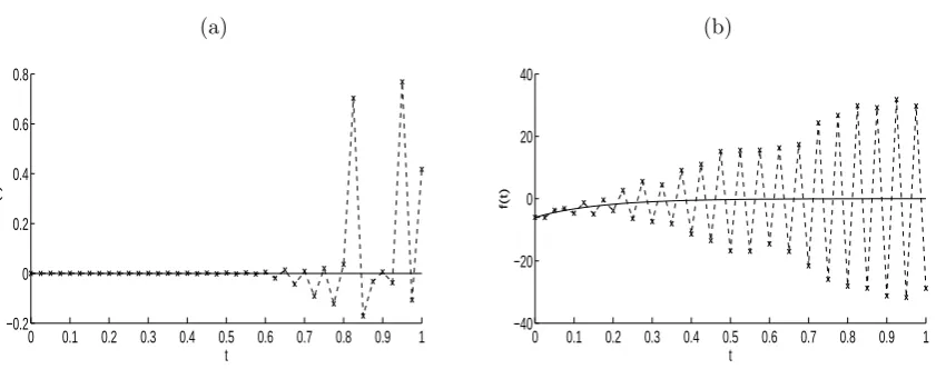
Figure 5: The exact (—) and numerical (- × -) solutions without regularization for: (a) b(t) and (b)f(t), for Example 1 withp= 1% noisy data.

0 1 2 3 4 5 6 7 8 10−3

10−2 10−1 100 101

Number of Iterations

Regularized objective function

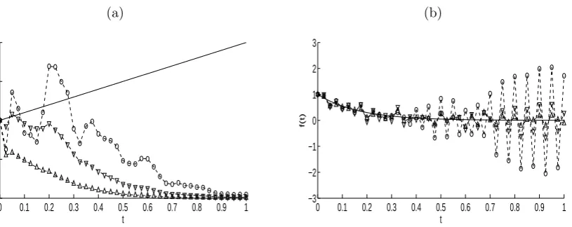
Figure 6: The objective function (27) with regularization parameters β1 = β2 = 10−5 (--),

β1 =β2 = 10−4 (-△-), β1 = β2 = 10−3 (-▽-) and β1 = 10−3, β2 = 10−4 (-◦-), for Example 1

withp= 1% noisy data.

(a)

0 0.1 0.2 0.3 0.4 0.5 0.6 0.7 0.8 0.9 1 −3

−2 −1 0 1 2 3x 10

−5

t

b(t)

(b)

0 0.1 0.2 0.3 0.4 0.5 0.6 0.7 0.8 0.9 1 −6

−4 −2 0 2

t

f(t)

Figure 7: The exact (—) and numerical solutions with regularization parametersβ₁ =β₂= 10−5

(--), β1 =β2= 10−4 (-△-), β1=β2 = 10−3 (-▽-) andβ1= 10−3,β2 = 10−4 (-◦-) for: (a)b(t)

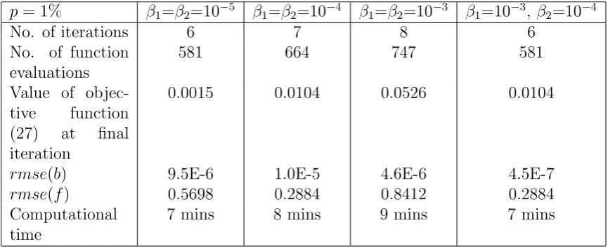
Table 2: Number of iterations, number of function evaluations, value of the objective function (27) at final iteration, the rmse values and the computational time, with regularization for Example 1 withp= 1% noisy data.

p= 1% β1=β2=10−5 β1=β2=10−4 β1=β2=10−3 β1=10−3, β2=10−4

No. of iterations 6 7 8 6

No. of function evaluations

581 664 747 581

Value of

objec-tive function

(27) at final

iteration

0.0015 0.0104 0.0526 0.0104

rmse(b) 9.5E-6 1.0E-5 4.6E-6 4.5E-7

rmse(f) 0.5698 0.2884 0.8412 0.2884

Computational time

7 mins 8 mins 9 mins 7 mins

5.2

Example 2

In this example, we consider solving the second inverse problem given by equations (3)–(7) with unknown coefficients f(t) and d(t)≥0, and the following input data:

b(x, t) = 1, g(x, t) = (5−t)x 3

ℓ2 −3x

2_{+ (1 +t)x+ℓ}2_{, (x, t)∈Q}

T, (50)

and a, ϕ, ω, φ, andψ given by equations (45)–(47).

One can easily check the the conditions of Theorem 2 are satisfied; in particular

∆1(t) =

∫ ℓ

−ℓ

g(x, t) (ω(x)ψ(t) +ω′

(x)φ(t))dx

= 4096e

−6t/ℓ2

ℓ14

11025 ≥

4096e−6T /ℓ2

ℓ14

11025 =:δ1 >0, t∈[0, T],

and therefore the inverse problem has at most one solution in the class of functions (15). In fact, it can easily be checked by direct substitution that the analytical solution is given by

d(t) = 1 +t

ℓ2 , f(t) = e

−6t

ℓ2, t ∈[0, T], (51)

and u(x, t) is given by (49).

As in Example 5.1, we takeℓ =T = 1 and employ the FDM with M=N=40. Remark that from (39) and (43) we obtain thatf(0)=1 andd(0)=1. So, we take the initial guesses

100 101 102 10−8

10−6 10−4 10−2

Number of Iterations

Unregularized objective function

p=0 p=1%

Figure 8: The objective function (28) without regularization, for Example 2 with exact data andp= 1% noisy data.

Figures 8 and 9 illustrate the convergence of the unregularized objective function (28) withβ2 =β3 = 0 and the corresponding recovered coefficientsd(t) and f(t), respectively, for exact datap= 0 and forp= 1% noisy data. First, from Figure 8 it can be seen that for exact data the unregularized objective function decreases rapidly in about 26 iterations to a low threshold ofO(10−8_{). However, for p= 1% noisy data, the number of iterations} necessary to achieve the required degree of convergence with respect to the tolerance chosen increases to 191, see also the second column of Table 3 where, in particular, one can observe the long computational time recorded to be in excess of 4 hours. In Figure 9, reasonable good retrievals for the unknown coefficients can be observed for exact data, but the instability clearly manifests for noisy data. In order to stabilise the solution for noisy data, as in Example 5.1, regularization needs to be included in the functional (28) which is minimized.

(a)

0 0.1 0.2 0.3 0.4 0.5 0.6 0.7 0.8 0.9 1 0

0.5 1 1.5 2 2.5

t

d(t)

(b)

0 0.1 0.2 0.3 0.4 0.5 0.6 0.7 0.8 0.9 1 −4

−2 0 2 4 6

t

f(t)

Figure 9: The exact (—) and numerical solutions without regularization for: (a) d(t) and (b)

0 5 10 15 20 25 30 35 40 45 50 10−4

10−3 10−2 10−1 100 101

Number of Iterations

Regularized objective function

Figure 10: The objective function (28) with regularization parameters β2 =β3 = 10−4 (-△-),

β2=β3 = 10−5 (-▽-) andβ2 =β3= 10−6 (-◦-), for Example 2 with p= 1% noisy data.

(a)

0 0.1 0.2 0.3 0.4 0.5 0.6 0.7 0.8 0.9 1 0

0.5 1 1.5 2

t

d(t)

(b)

0 0.1 0.2 0.3 0.4 0.5 0.6 0.7 0.8 0.9 1 −3

−2 −1 0 1 2 3

t

f(t)

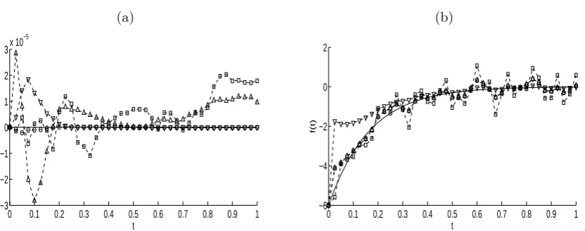
Figure 11: The exact (—) and numerical solutions with regularization parameters β2 =β3 =

10−4 _{(-△-), β}

2 = β3 = 10−5 (-▽-) and β2 = β3 = 10−6 (-◦-) for: (a) d(t) and (b) f(t), for

Example 2 withp= 1% noisy data.

Table 3: Number of iterations, number of function evaluations, value of the objective func-tion (28) at final iterafunc-tion, rmse values and the computational time, for various regularization parameters, for Example 2 withp= 1% noisy data.

p= 1% β2=β3=0 β2=β3=10−6 β2=β3=10−5 β2=β3=10−4

No. of iterations 191 46 22 11

No. of function evaluations 15936 3901 1909 996

Value of objective function (28) at final iteration

3E-5 0.0001 0.0004 0.0011

rmse(d) 0.6283 1.1731 1.3207 1.4409

rmse(f) 2.3165 1.0330 0.3127 0.1325

Computational time 4 hours 57 mins 28 mins 15 mins

when the input data (6) and (7) is contaminated with p = 1% noise. From this figure it can be remarked that a rapid convergent is achieved for each selection of regulariza-tion parameters. The corresponding exact and numerical soluregulariza-tions for d(t) and f(t) are presented in Figure 11 and other numerical features of the solutions are summarised in Table 3. First, by comparing Figures 9 and 11 clearly the stabilisation benefit of employ-ing regularization can be appreciated. It is also interestemploy-ing to remark from Table 3 that retrieving accurately and simultaneously both the coefficients d(t) and f(t) requires an appropriate choice of the regularization parameters β2 and β3, e.g. for β2 = β3 = 0 the recovery ofd(t) is accurate in the detriment of that of f(t), whilst for β2 =β3 = 10−4 the accuracy of the simultaneous recovery is viceversa. This situation has also been observed previously in cases where simultaneous identification of multiple coefficients has been at-tempted, [7, 9]. Therefore, a compromising but balancing choice would be to pickβ2 =β3 in between, say between 10−5 _{and 10}−4 _{as is common with ill-posed problems in which} acceptable candidate solutions are those in the region where the accuracy and stability portions meet/ intersect.

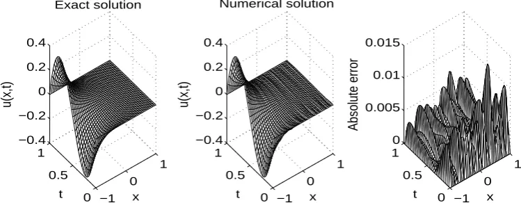
Finally, for completeness, the exact and numerical reconstructions for the temperature

u(x, t) are presented in Figure 12 and the absolute error between them is also included. From this figure it can be observed that a stable and accurate reconstruction is obtained.

−1 0

1

0 0.5 1 −0.4 −0.2 0 0.2 0.4

x Exact solution

t

u(x,t)

−1 0

1

0 0.5 1 −0.4 −0.2 0 0.2 0.4

x Numerical solution

t

u(x,t)

−1 0

1

0 0.5 1 0 0.005 0.01 0.015

x t

Absolute error

Figure 12: The exact (49) and numerical reconstructions for the temperature u(x, t) with regularization parametersβ1 =β2 = 10−5, for Example 2 with p= 1% noisy data.

6

Conclusions

A couple of inverse problems consisting of finding the time-dependent coefficients and the time-dependent heat source term in the parabolic heat equation with integral overdetermi-nation conditions have been numerically investigated. The MATLAB routine lsqnonlin

Acknowledgments

M.S. Hussein would like to thank the financial support received from the Higher Commit-tee for Education Development in Iraq (HCEDiraq) for pursuing his Ph.D at the University of Leeds. Some fruitful discussion with Professor V.L. Kamynin is also acknowledged.

References

[1] Aida-zade, K.R. and Rahimov, A.B. (2015) Solution to classes of inverse coefficient problems and problems with nonlocal conditions for parabolic equations,Differential Equations, 51, 83–93.

[2] Belge, M., Kilmer, M. and Miller, E.L. (2002) Efficient determination of multiple regularization parameters in a generalized L-curve framework,Inverse Problems,18, 1161–1183.

[3] Budak, B.M. and Iskenderov, A.D. (1967) On a class of boundary value problems with unknown coefficients, Soviet Math. Dokl., 8, 786–789.

[4] Cannon, J.R. (1984) The One-dimensional Heat Equation, Addison-Wesley, Menlo Park, California.

[5] Cannon, J.R. and Hoek, J. (1986) Diffusion subject to the specification of mass,

Journal of Mathematical Analysis and Applications,115, 517–529.

[6] Cannon, J.R. and Lin, Y. (1988) Determination of a parameter p(t) in some quasi-linear parabolic differential equations,Inverse Problems,4, 35–45.

[7] Hazanee, A. and Lesnic, D. (2013) Reconstruction of an additive space- and time-dependent heat source,European Journal of Computational Mechanics,22, 304–329.

[8] Hussein, M.S., Lesnic, D. and Ivanchov, M.I. (2014) Simultaneous determination of time-dependent coefficients in the heat equation, Computers and Mathematics with Applications, 67, 1065-1091.

[9] Hussein, M.S., Lesnic, D. and Ismailov, M.I. (2015) An inverse problem of finding the time-dependent diffusion coefficient from an integral condition, Mathematical Methods in the Applied Sciences, doi: 10.1002/mma.3482.

[10] Ionkin, N.I. (1977) Solution of a boundary-value problem in heat conduction with a nonclassical boundary condition,Differential Equations, 13, 204-211.

[11] Ivanchov, M.I. and Pabyrivs’ka, N.V. (2001) Simultaneous determination of two co-efficients of a parabolic equation in the case of nonlocal and integral conditions,

Ukrainian Mathematical Journal, 53, 674–684.

[12] Ivanchov, M.I. Inverse Problems for Equations of Parabolic Type, VNTL Publishers, Lviv, Ukraine, 2003.

[14] Kamynin, V.L. (2014) Inverse problem of simultaneously determining the right-hand side and the coefficient of a lower order derivative for a parabolic equation on the plane,Differential Equations, 50, 792–804.

[15] Kamynin, V.L. (2015) Inverse problem of simultaneous determination of the time-dependent right-hand side term and the coefficient in a parabolic equation, Lecture Notes in Computer Science, 9045, 218-225.

[16] Ladyzenskaja, O.A., Solonnikov, V.A. and Uralceva, N.N. Linear and Quasi-linear Equations of Parabolic Type, Translations of Mathematical Monographs 23, Provi-dence, R.I., American Mathematical Society, 1968.

[17] Mathwoks R2012 Documentation Optimization Toolbox-Least Squares (Model Fit-ting) Algorithms, available from www.mathworks.com/help/toolbox/optim/ug /brnoybu.html.